FNETS: Factor-Adjusted Network Estimation and Forecasting for High-Dimensional Time Series

Abstract

We propose FNETS, a methodology for network estimation and forecasting of high-dimensional time series exhibiting strong serial- and cross-sectional correlations. We operate under a factor-adjusted vector autoregressive (VAR) model which, after accounting for pervasive co-movements of the variables by common factors, models the remaining idiosyncratic dynamic dependence between the variables as a sparse VAR process. Network estimation of FNETS consists of three steps: (i) factor-adjustment via dynamic principal component analysis, (ii) estimation of the latent VAR process via ${\mathcal{l}}_1$-regularized Yule-Walker estimator, and (iii) estimation of partial correlation and long-run partial correlation matrices. In doing so, we learn three networks underpinning the VAR process, namely a directed network representing the Granger causal linkages between the variables, an undirected one embedding their contemporaneous relationships and finally, an undirected network that summarizes both lead-lag and contemporaneous linkages. In addition, FNETS provides a suite of methods for forecasting the factor-driven and the idiosyncratic VAR processes. Under general conditions permitting tails heavier than the Gaussian one, we derive uniform consistency rates for the estimators in both network estimation and forecasting, which hold as the dimension of the panel and the sample size diverge. Simulation studies and real data application confirm the good performance of FNETS.

Keywords:

• Dynamic factor model
• Forecasting
• Network estimation
• Vector autoregression

1 Introduction

Vector autoregressive (VAR) models are popularly adopted for time series analysis in economics and finance. Fitting a VAR model to the data enables inferring dynamic interdependence between the variables as well as forecasting the future. VAR models are particularly appealing for network analysis since estimating the nonzero elements of the VAR parameter matrices, a.k.a. transition matrices, recovers directed edges between the components of vector time series in a Granger causality network. In addition, by estimating a precision matrix (inverse of the covariance matrix) of the VAR innovations, we can also define a network capturing contemporaneous linear dependencies. For the network interpretation of VAR modeling, see for example, Dahlhaus (2000), Eichler (2007), Billio et al. (2012), Ahelegbey, Billio, and Casarin (2016), Barigozzi and Brownlees (2019), Guðmundsson and Brownlees (2021), and Uematsu and Yamagata (2023).

Estimation of VAR models quickly becomes a high-dimensional problem as the number of parameters grows quadratically with the dimensionality. There is a mature literature on estimation of high-dimensional VAR models under the sparsity (Hsu, Hung, and Chang 2008; Basu and Michailidis 2015; Han, Lu, and Liu 2015; Kock and Callot 2015; Nicholson et al. 2020; Krampe and Paparoditis 2021; Masini, Medeiros, and Mendes 2022; Adamek, Smeekes, and Wilms 2023) and low-rank plus sparsity (Basu, Li, and Michailidis 2019) assumptions, see also BańburaBańbura, Giannone, and Reichlin (2010) for a Bayesian approach. In all above, either explicitly or implicitly, the spectral density of the time series is required to have eigenvalues which are uniformly bounded over frequencies. Indeed, this condition is crucial for controlling the deviation bounds involved in theoretical investigation of regularized estimators.

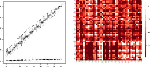
Lin and Michailidis (2020) observe that for VAR processes, this assumption restricts the parameters to be either dense but small in their magnitude (which makes their estimation using the shrinkage-based methods challenging) or highly sparse, while Giannone, Lenza, and Primiceri (2021) note the difficulty of identifying sparse predictive representations in many economic applications. Moreover, some datasets typically exhibit strong serial and cross-sectional correlations and violate the bounded spectrum assumption. The left panel of Figure 1 provides an illustration of this phenomenon; with the increase of dimensionality, a volatility panel dataset (see Section 5.3 for its description) exhibits a linear increase in the leading eigenvalue of the estimate of its spectral density matrix at frequency 0 (i.e., long-run covariance). The right panel visualizes the outcome from fitting a VAR(5) model to the same dataset without making any adjustment of the strong correlations (see the caption for further details), from which we cannot infer meaningful, sparse pairwise relationship.

Fig. 1 Left: The two largest eigenvalues (y-axis) of the long-run covariance matrix estimated from the volatility panel analyzed in Section 5.3 (March 2008 to March 2009, n = 252) with subsets of cross-sections randomly sampled 100 times for each given dimension $p\in \{5,\dots ,46\}$ (x-axis). Right: logged and truncated p-values (truncation level chosen by Bonferroni correction with the significance level 0.1) from fitting a VAR(5) model to the same dataset using ridge regression and generating p-values corresponding to each coefficient as described in Cule, Vineis, and De Iorio (2011). For each pair of variables (corresponding tickers given in x- and y-axes), the minimum p-value over the five lags is reported.

In this article, we propose to model high-dimensional time series by means of a factor-adjusted VAR approach, which simultaneously accounts for strong serial and cross-sectional correlations attributed to factors, as well as sparse, idiosyncratic correlations among the variables that remain after factor adjustment. We take the most general approach to factor modeling based on the generalized dynamic factor model, where factors are dynamic in the sense that they are allowed to have not only contemporaneous but also lagged effects on the variables (Forni et al. 2000). We propose FNETS, a suite of tools accompanying the model for estimation and forecasting with a particular focus on network analysis, which addresses the challenges arising from the latency of the VAR process as well as high dimensionality.

We make the following methodological and theoretical contributions.

1. We propose an ${\mathcal{l}}_1$-regularized Yule-Walker estimation method for estimating the factor-adjusted, idiosyncratic VAR, while permitting the number of nonzero parameters to slowly grow with the dimensionality. Estimating the VAR parameters and the inverse of the innovation covariance, and then combining them allow us to define three networks underlying the latent VAR process, namely a direct network representing Granger causal linkages, an undirected one underpinning their contemporaneous relationships, as well as an undirected network summarizing both. Under general conditions permitting weak factors and heavier tails than the sub-Gaussian one, we show the consistency of FNETS in estimating the edge sets of these networks, which holds uniformly over all p² entries of the networks (Propositions 3.3 and 3.5).

2. We provide new consistency rates for the estimation and forecasting approaches considered by Forni et al. (2005, 2017), which hold uniformly for the entire cross-sections of p-dimensional time series (Propositions 4.1 and B.2). In doing so, we establish uniform consistency of the estimators of high-dimensional spectral density matrices of the factor-driven and the idiosyncratic components, extending the results of Zhang and Wu (2021) to the presence of latent factors.

Our approach differs from the existing ones for factor-adjusted regression problems (Fan, Ke, and Wang 2020; Fan, Masini, and Medeiros 2021; Fan, Lou, and Yu 2023; Krampe and Margaritella 2021), as (i) it allows for the presence of dynamic factors, thus including all possible dynamic linear co-dependencies, and (ii) it relies only on the estimators of the autocovariances of the latent idiosyncratic process, and avoids estimating the entire latent process and controlling the errors arising from such a step, which increase with the sample size. The price to pay for the generality of the factor modeling in (i), is an extra term appearing in the rate of consistency which represents the bandwidth for spectral density estimation required for factor-adjustment in the frequency domain. We make explicit the role played by this bandwidth in the theoretical results, and also present the results under a more restricted static factor model for ease of comparison. We mention two more differences between this article and Fan, Masini, and Medeiros (2021) and Fan, Lou, and Yu (2023). First, they additionally consider the problem of testing hypotheses on the idiosyncratic covariance and the adequacy of factor/sparse regression, while we focus on network estimation. Second, their methods accommodate models for the idiosyncratic component other than VAR.

FNETS is another take the popular low-rank plus sparsity modeling framework in the high-dimensional learning literature, Also, it is in line with a frequently adopted practice in financial time series analysis where factor-driven common components representing the systematic sources of risk, are removed prior to inferring a network structure via (sparse) regression modeling and identifying the most central nodes representing the systemic sources of risk (Diebold and Y ilmaz 2014; Barigozzi and Brownlees 2019). We provide a rigorous theoretical treatment of this empirical approach by accounting for the effect of the factor-adjustment step on the second step regression.

The rest of the article is organized as follows. Section 2 introduces the factor-adjusted VAR model. Sections 3 and 4 describe the network estimation and forecasting methodologies comprising FNETS, respectively, and provide their theoretical consistency. In Section 5, we demonstrate the good estimation and forecasting performance of FNETS on a panel of volatility measures. Section 6 concludes the article, and all the proofs and complete simulation results are presented in Supplementary Appendix. The R software fnets implementing FNETS is available from CRAN (Barigozzi, Cho, and Owens 2023).

Notations

By $\mathbf{I},\mathbf{O}$, and $\mathbf{0}$, we denote an identity matrix, a matrix of zeros, and a vector of zeros whose dimensions depend on the context. For a matrix $\mathbf{A}=[a_{ii\prime }, 1\le i\le m, 1\le i\prime \le n]$, we denote by ${\mathbf{A}}^{\top }$ its transpose. The element-wise ${\mathcal{l}}_{\infty },{\mathcal{l}}_0,{\mathcal{l}}_1$ and ${\mathcal{l}}_2$-norms are denoted by $|\mathbf{A}{|}_{\infty }={\max }_{1\le i\le m}{\max }_{1\le i\prime \le n}|a_{ii\prime }|$, $|\mathbf{A}{|}_0={\sum }_{i=1}^m{\sum }_{i\prime =1}^n{\mathbb{I}}_{\{a_{ii\prime }\ne 0\}}$, $|\mathbf{A}{|}_1={\sum }_{i=1}^m{\sum }_{i\prime =1}^n|a_{ii\prime }|$ and $|\mathbf{A}{|}_2=\sqrt{{\sum }_{i=1}^m{\sum }_{i\prime =1}^n|a_{ii\prime }{|}^2}$. The Frobenius, spectral, induced L₁ and $L_{\infty }$-norms are denoted by $\left|\right|\mathbf{A}|{|}_F=|\mathbf{A}{|}_2$, $\left|\right|\mathbf{A}\left|\right|=\sqrt{{\Lambda }_{\max }({\mathbf{A}}^{\top }\mathbf{A})}$ (with ${\Lambda }_{\max }(\mathbf{A})$ and ${\Lambda }_{\min }(\mathbf{A})$ denoting its largest and smallest eigenvalues in modulus), $\left|\right|\mathbf{A}|{|}_1={\max }_{1\le i\prime \le n}{\sum }_{i=1}^m|a_{ii\prime }|$ and $\left|\right|\mathbf{A}|{|}_{\infty }={\max }_{1\le i\le n}{\sum }_{i\prime =1}^m|a_{ii\prime }|$. Let ${\mathbf{A}}_{i·}$ and ${\mathbf{A}}_{·k}$ denote the ith row and the kth column of $\mathbf{A}$. For two real numbers, set $a\vee b=\max (a,b)$ and $a\wedge b=\min (a,b)$. Given two sequences $\left\{a_n\right\}$ and $\left\{b_n\right\}$, we write $a_n=O(b_n)$ if, for some finite constant C > 0 there exists $N\in {\mathbb{N}}_0=\mathbb{N}\cup \left\{0\right\}$ such that $\left|a_n\right||b_n{|}^{-1}\le C$ for all $n\ge N$; we denote by O_P the stochastic boundedness. We write $a_n\asymp b_n$ when $a_n=O(b_n)$ and $b_n=O(a_n)$. Throughout, L denotes the lag operator and $\iota =\sqrt{-1}$. Finally, ${\mathbb{I}}_{\mathcal{A}}=1$ if the event $\mathcal{A}$ takes place and 0 otherwise.

2 Factor-Adjusted Vector Autoregressive Model

Consider a zero-mean, second-order stationary p-variate process ${\mathbf{X}}_t={(X_{1t},\dots ,X_{pt})}^{\top },1\le t\le n$, which is decomposed into the sum of two latent components: a factor-driven, common component ${\mathit{\chi }}_t={({\chi }_{1t},\dots ,{\chi }_{pt})}^{\top }$, and an idiosyncratic component ${\mathit{\xi }}_t={({\xi }_{1t},\dots ,{\xi }_{pt})}^{\top }$ modeled as a VAR process. That is, ${\mathbf{X}}_t={\mathit{\chi }}_t+{\mathit{\xi }}_t$ where (1) $${\mathit{\chi }}_t=\mathcal{B}(L){\mathit{u}}_t=\sum _{\mathcal{l}=0}^{\infty }{\mathit{B}}_{\mathcal{l}}{\mathit{u}}_{t-\mathcal{l}}\text{ with }{\mathit{u}}_t={(u_{1t},\dots ,u_{qt})}^{\top },\hspace{1em}\text{and}$$(1) (2) $$\mathcal{A}(L){\mathit{\xi }}_t={\mathit{\xi }}_t-\sum _{\mathcal{l}=1}^d{\mathit{A}}_{\mathcal{l}}{\mathit{\xi }}_{t-\mathcal{l}}={\mathbf{\Gamma }}^{1/2}{\mathit{\epsilon }}_t\text{ with }{\mathit{\epsilon }}_t={({\epsilon }_{1t},\dots ,{\epsilon }_{pt})}^{\top }.$$(2)

In (1), the latent random vector ${\mathbf{u}}_t$, referred to as the vector of common factors or common shocks, is assumed to satisfy $\mathsf{E}({\mathbf{u}}_t)=\mathbf{0}$ and $\mathsf{cov}({\mathbf{u}}_t)={\mathbf{I}}_q$, and are loaded on each χ_it via square summable, one-sided filters ${\mathcal{B}}_{ij}(L)={\sum }_{\mathcal{l}=0}^{\infty }{B}_{\mathcal{l},ij}{L}^{\mathcal{l}}$, where ${\mathbf{B}}_{\mathcal{l}}=[B_{\mathcal{l},ij}, 1\le i\le p, 1\le j\le q]\in {\mathbb{R}}^{p\times q}$. This defines the generalized dynamic factor model (GDFM) proposed by Forni et al. (2000) and Forni and Lippi (2001), which provides the most general approach to high-dimensional time series factor modeling.

In (2), the idiosyncratic component ${\mathit{\xi }}_t$ is modeled as a VAR(d) process for some finite positive integer d, with innovations ${\mathbf{\Gamma }}^{1/2}{\mathit{\epsilon }}_t$ where $\mathbf{\Gamma }\in {\mathbb{R}}^{p\times p}$ is some positive definite matrix and ${\mathbf{\Gamma }}^{1/2}$ its symmetric square root matrix, and $\mathsf{E}({\mathit{\epsilon }}_t)=\mathbf{0}$ and $\mathsf{cov}({\mathit{\epsilon }}_t)={\mathbf{I}}_p$. We assume that ${\mathit{\xi }}_t$ is causal (see Assumption 2.3(i)), that is, it admits the Wold representation: (3) $${\mathit{\xi }}_t=\mathcal{D}(L){\mathbf{\Gamma }}^{1/2}{\mathit{\epsilon }}_t=\sum _{\mathcal{l}=0}^{\infty }{\mathit{D}}_{\mathcal{l}}{\mathbf{\Gamma }}^{1/2}{\mathit{\epsilon }}_{t-\mathcal{l}}\text{with}\mathcal{D}(L)={\mathcal{A}}^{-1}(L),$$(3) such that ${\mathbf{\Gamma }}^{1/2}{\mathit{\epsilon }}_t$ is seen as a vector of idiosyncratic shocks loaded on each ξ_it via square summable, one-sided filters ${\mathcal{D}}_{ik}(L)={\sum }_{\mathcal{l}=0}^{\infty }{D}_{\mathcal{l},ik}{L}^{\mathcal{l}}$ where ${\mathbf{D}}_{\mathcal{l}}=[D_{\mathcal{l},ik}, 1\le i,k\le p]$. After accounting for the dominant cross-sectional dependence in the data (both contemporaneous and lagged) by factors, it is reasonable to assume that the dependences left in ${\mathit{\xi }}_t$ are weak and, therefore, that the VAR structure is sufficiently sparse. Discussion on the precise requirement on the sparsity of ${\mathbf{A}}_{\mathcal{l}}, 1\le \mathcal{l}\le d$, and ${\mathbf{\Gamma }}^{-1}$ is deferred to Section 3.

Remark 2.1.

A special case of the GDFM is the popularly adopted static factor model where the factors are loaded only contemporaneously (see e.g., Stock and Watson 2002; Bai 2003; Fan, Liao, and Mincheva 2013). This is formalized in Assumption 4.1, where we consider forecasting under a static representation. A sufficient condition to obtain a static representation from the GDFM in (1), is to assume $\mathcal{B}(L)={\sum }_{\mathcal{l}=0}^s{\mathbf{B}}_{\mathcal{l}}{L}^{\mathcal{l}}$ for some finite integer $s\ge 0$. For example, if s = 0, the model reduces to ${\mathit{\chi }}_t={\mathbf{B}}_0{\mathbf{u}}_t$ while if s > 0, it can be written as ${\mathit{\chi }}_t=\mathbf{\Lambda }{\mathbf{F}}_t$ with $\mathbf{\Lambda }=[{\mathbf{B}}_{\mathcal{l}}, 0\le \mathcal{l}\le s]$ and ${\mathbf{F}}_t={({\mathbf{u}}_t^{\top },\dots ,{\mathbf{u}}_{t-s}^{\top })}^{\top }$. Under the static factor model, ${\mathbf{X}}_t$ admits a factor-augmented VAR representation (see Remark 4.1).

In the remainder of this section, we list the assumptions required for identification and estimation of (1)–(2). Since ${\mathit{\chi }}_t$ and ${\mathit{\xi }}_t$ are latent, some assumptions are required to ensure their (asymptotic) identifiability which are made in the frequency domain. Denote by ${\mathbf{\Sigma }}_x(\omega )$ the spectral density matrix of ${\mathbf{X}}_t$ at frequency $\omega \in [-\pi ,\pi ]$, and ${\mu }_{x,j}(\omega )$ its dynamic eigenvalues which are real-valued and ordered in the decreasing order. We similarly define ${\mathbf{\Sigma }}_{\chi }(\omega ),{\mu }_{\chi ,j}(\omega ),{\mathbf{\Sigma }}_{\xi }(\omega )$ and ${\mu }_{\xi ,j}(\omega )$.

Assumption 2.1.

There exist a positive integer $p_0\ge 1$, constants ${\rho }_j\in (3/4,1]$ with ${\rho }_1\ge \cdots \ge {\rho }_q$, and pairs of continuous functions $\omega \mapsto {\alpha }_{\chi ,j}(\omega )$ and $\omega \mapsto {\beta }_{\chi ,j}(\omega )$ for $\omega \in [-\pi ,\pi ]$ and $1\le j\le q$, such that for all $p\ge p_0$, $$\begin{array}{c}{\beta }_{\chi ,1}(\omega )\ge \frac{{\mu }_{\chi ,1}(\omega )}{p^{{\rho }_1}}\ge {\alpha }_{\chi ,1}(\omega )>\cdots >{\beta }_{\chi ,q}(\omega )\\ \ge \frac{{\mu }_{\chi ,q}(\omega )}{p^{{\rho }_q}}\ge {\alpha }_{\chi ,q}(\omega )>0.\end{array}$$

Under the assumption, if ${\rho }_j=1$ for all $1\le j\le q$, then we are in presence of q factors that are equally pervasive for the whole cross-section. The left panel of Figure 1 depicts the case when ${\rho }_1=1$. If ${\rho }_j<1$ for some j, we permit the presence of “weak” factors and our theoretical analysis explicitly reflects this; see, for example, Onatski (2012) and Freyaldenhoven (2021) for static factor models permitting weak factors. When weak factors are present, the ordering of the variables becomes important as $p\to \infty$, whereas the case of linearly diverging factor strengths is compatible with completely arbitrary cross-sectional ordering. The requirement that ${\rho }_j>3/4$ is a minimal one, and generally larger values of ρ_j are required as the dimensionality increases and heavier tails are permitted as discussed later.

Assumptions 2.2 and 2.3 are made to control the serial dependence in ${\mathbf{X}}_t$.

Assumption 2.2.

There exist some constants $\Xi >0$ and $\varsigma >2$ such that for all $\mathcal{l}\ge 0$, $$\begin{array}{c}\underset{{}_{1\le i\le p}}{\max }|{\mathit{B}}_{\mathcal{l},i·}{|}_2\le \Xi {(1+\mathcal{l})}^{-\varsigma }\hspace{1em}\text{and}\\ {\left(\sum _{j=1}^q|{\mathit{B}}_{\mathcal{l},·j}{|}_{\infty }^2\right)}^{1/2}\le \Xi {(1+\mathcal{l})}^{-\varsigma }.\end{array}$$

Assumption 2.3.

1. d is a finite positive integer and $\det (\mathcal{A}(z))\ne 0$ for all $\left|z\right|\le 1$.

2. There exist some constants $0<m_{\epsilon }\le M_{\epsilon }$ such that $\left|\right|\mathbf{\Gamma }\left|\right|\le M_{\epsilon }$ and ${\Lambda }_{\min }(\mathbf{\Gamma })\ge m_{\epsilon }$.

3. There exist a constant $m_{\xi }>0$ such that $\underset{\omega \in [-\pi ,\pi ]}{\inf }{\mu }_{\xi ,p}(\omega )\ge m_{\xi }$.

4. There exist some constants $\Xi >0$ and $\varsigma >2$ such that for all $\mathcal{l}\ge 0$, $$\begin{array}{c}\left|D_{\mathcal{l},ik}\right|\le C_{ik}{(1+\mathcal{l})}^{-\varsigma }\text{ with }\\ \hspace{1em}\max \left\{\mathrm{}\underset{{}_{1\le k\le p}}{\max }\sum _{i=1}^p{C}_{ik}, \underset{{}_{1\le i\le p}}{\max }\sum _{k=1}^p{C}_{ik},\underset{{}_{1\le i\le p}}{\max }\sqrt{\sum _{k=1}^p{C}_{ik}^2}\mathrm{}\right\}\le \Xi .\end{array}$$

Assumption 2.3 (i) and (ii) are standard in the literature (Lütkepohl 2005) and imply that ${\mathit{\xi }}_t$ is causal and has finite and nonzero covariance. Under Assumptions 2.2 and 2.3 (iv) (imposed on the Wold decomposition of ${\mathit{\xi }}_t$ in (3)), the serial dependence in ${\mathbf{X}}_t$ decays at an algebraic rate. Further, we obtain a uniform bound for ${\mu }_{\xi ,j}(\omega )$ under Assumption 2.3 (iv):

Proposition 2.1.

Under Assumption 2.3, uniformly over all $\omega \in [-\pi ,\pi ]$, there exists some constant $B_{\xi }>0$ depending only on $M_{\epsilon }$, Ξ and Ϛ, defined in Assumption 2.3 (iii) and (iv), such that $\underset{\omega \in [-\pi ,\pi ]}{\sup }{\mu }_{\xi ,1}(\omega )\le B_{\xi }$.

Remark 2.2.

Proposition 2.1 and Assumption 2.3 (iii) jointly establish the uniform boundedness of ${\mu }_{\xi ,1}(\omega )$ and ${\mu }_{\xi ,p}(\omega )$, which is commonly assumed in the literature on high- dimensional VAR estimation via ${\mathcal{l}}_1$-regularization. A sufficient condition for Assumption 2.3 (iii) is that $\max \left\{{\max }_{1\le i\le p}{\sum }_{\mathcal{l}=1}^d\right|{\mathbf{A}}_{\mathcal{l},i·}{|}_1,{\max }_{1\le j\le p}{\sum }_{\mathcal{l}=1}^d\left|{\mathbf{A}}_{\mathcal{l},·j}{|}_1\right\} \le \Xi$ for some constant $\Xi >0$ (Basu and Michailidis 2015). Further, when for example, d = 1, Assumption 2.3 (iv) follows if $|{\mathbf{A}}_1{|}_{\infty }\le \gamma <1$ since $\max (|\left|{\mathbf{D}}_{\mathcal{l}}\right|{|}_1,\left|\right|{\mathbf{D}}_{\mathcal{l}}|{|}_{\infty })\le \Xi {\gamma }^{\mathcal{l}}$ with ${\mathbf{D}}_{\mathcal{l}}={\mathbf{A}}_1^{\mathcal{l}}$.

The two latent components ${\mathit{\chi }}_t$ and ${\mathit{\xi }}_t$, and the number of factors q, are identified thanks to the large gap between the eigenvalues of their spectral density matrices, which follows from Assumption 2.1 and Proposition 2.1. Then by Weyl’s inequality, the qth dynamic eigenvalue ${\mu }_{x,q}(\omega )$ diverges almost everywhere in $[-\pi ,\pi ]$ as $p\to \infty$, whereas ${\mu }_{x,q+1}(\omega )$ is uniformly bounded for any $p\in \mathbb{N}$ and ω. This property is exploited in the FNETS methodology as later described in Section 3.2. It is worth stressing that Assumption 2.1 and Proposition 2.1 jointly constitute both a necessary and sufficient condition for the process ${\mathbf{X}}_t$ to admit the dynamic factor representation in (1), see Forni and Lippi (2001).

Finally, we characterize the common and idiosyncratic innovations.

Assumption 2.4.

1. ${\left\{{\mathbf{u}}_t\right\}}_{t\in \mathbb{Z}}$ is a sequence of zero-mean, q-dimensional martingale difference vectors with $\mathsf{cov}({\mathbf{u}}_t)={\mathbf{I}}_q$, and u_it and u_jt are independent for all $1\le i,j\le q$ with $i\ne j$ and all $t\in \mathbb{Z}$.

2. ${\left\{{\mathit{\epsilon }}_t\right\}}_{t\in \mathbb{Z}}$ is a sequence of zero-mean, p-dimensional martingale difference vectors with $\mathsf{cov}({\mathit{\epsilon }}_t)={\mathbf{I}}_p$, and ${\epsilon }_{it}$ and ${\epsilon }_{jt}$ are independent for all $1\le i,j\le p$ with $i\ne j$ and all $t\in \mathbb{Z}$.

3. $\mathsf{E}(u_{jt}{\epsilon }_{it\prime }) = 0$ for all $1\le j\le q,1\le i\le p$ and $t,t\prime \in \mathbb{Z}$.

4. There exist some constants $\nu >4$ and ${\mu }_{\nu }>0$ such that $\max \left\{{\max }_{1\le j\le q}\mathsf{E}(|u_{jt}{|}^{\nu }),{\max }_{1\le i\le p}\mathsf{E}(|{\epsilon }_{it}{|}^{\nu })\right\}\le {\mu }_{\nu }$.

Assumption 2.4 (i) and (ii) allow the common and idiosyncratic innovations to be sequences of martingale differences, relaxing the assumption of serial independence found in Forni et al. (2017). Condition (iii) is standard in the factor modeling literature. Under (iv), we require that the innovations have $\nu >4$ moments, which is considerably weaker than Gaussian or sub-Weibull tails assumed in the literature on VAR modeling of high-dimensional time series (Basu and Michailidis 2015; Kock and Callot 2015; Wong, Li, and Tewari 2020; Krampe and Paparoditis 2021; Masini, Medeiros, and Mendes 2022). Similar approaches to ours, based only on moment conditions, are found in Wu and Wu (2016) who investigate the Lasso performance in deterministic designs under functional dependence, and Adamek, Smeekes, and Wilms (2023) who assume instead near-epoch-dependence. In Appendix F, we separately consider the case when ${\mathbf{u}}_t$ and ${\mathit{\epsilon }}_t$ are Gaussian for the sake of comparison.

3 Network Estimation via FNETS

3.1 Networks Underpinning Factor-Adjusted VAR Processes

Under the latent VAR model in (2), we can define three types of networks underpinning the interconnectedness of ${\mathbf{X}}_t$ after factor adjustment (Barigozzi and Brownlees 2019).

Let $\mathcal{V}=\{1,\dots ,p\}$ denote the set of vertices representing the p time series. First, the transition matrices ${\mathbf{A}}_{\mathcal{l}}=[A_{\mathcal{l},ii\prime }, 1\le i,i\prime \le p]$, encode the directed network ${\mathcal{N}}^{\mathrm{G}}=(\mathcal{V},{\mathcal{E}}^{\mathrm{G}})$ representing Granger causal linkages, with (4) $${\mathcal{E}}^{\mathrm{G}}=\left\{(i,i\prime )\in \mathcal{V}\times \mathcal{V}: A_{\mathcal{l},ii\prime }\ne 0\text{ for some }1\le \mathcal{l}\le d\right\}$$(4) as the set of edges. Here, the presence of an edge $(i,i\prime )\in {\mathcal{E}}^{\mathrm{G}}$ indicates that ${\xi }_{i\prime ,t-\mathcal{l}}$ Granger causes ξ_it at some lag $1\le \mathcal{l}\le d$.

The second network contains undirected edges representing contemporaneous dependence between VAR innovations ${\mathbf{\Gamma }}^{1/2}{\mathit{\epsilon }}_t$, denoted by ${\mathcal{N}}^{\mathrm{C}}=(\mathcal{V},{\mathcal{E}}^{\mathrm{C}})$; we have $(i,i\prime )\in {\mathcal{E}}^{\mathrm{C}}$ iff the partial correlation between the ith and $i\prime$th elements of ${\mathbf{\Gamma }}^{1/2}{\mathit{\epsilon }}_t$ is nonzero. Specifically, letting ${\mathbf{\Gamma }}^{-1}=\Delta =[{\delta }_{ii\prime }, 1\le i,i\prime \le p]$, the set of edges is given by (5) $${\mathcal{E}}^{\mathrm{C}}=\left\{(i,i\prime )\in \mathcal{V}\times \mathcal{V}: i\ne i\prime \text{ and }-\frac{{\delta }_{ii\prime }}{\sqrt{{\delta }_{ii}·{\delta }_{i\prime i\prime }}}\ne 0\right\}.$$(5)

Finally, we summarize the aforementioned lead-lag and contemporaneous relations between the variables in a single, undirected network ${\mathcal{N}}^{\mathrm{L}}=(\mathcal{V},{\mathcal{E}}^{\mathrm{L}})$ by means of the long-run partial correlations of ${\mathit{\xi }}_t$. Let $\mathbf{\Omega }=[{\omega }_{ii\prime }, 1\le i,i\prime \le p]$ denote the long-run partial covariance matrix of ${\mathit{\xi }}_t$, that is $\mathbf{\Omega }={({\mathbf{\Sigma }}_{\xi }(0))}^{-1}=2\pi {\mathcal{A}}^{\top }(1)\Delta \mathcal{A}(1)$ under (2). Then, the set of edges of ${\mathcal{N}}^{\mathrm{L}}$ is (6) $${\mathcal{E}}^{\mathrm{L}}=\left\{(i,i\prime )\in \mathcal{V}\times \mathcal{V}: i\ne i\prime \text{ and }-\frac{{\omega }_{ii\prime }}{\sqrt{{\omega }_{ii}·{\omega }_{i\prime i\prime }}}\ne 0\right\}.$$(6)

Generally, ${\mathcal{E}}^{\mathrm{L}}$ is greater than ${\mathcal{E}}^{\mathrm{G}}\cup {\mathcal{E}}^{\mathrm{C}}$, see Appendix C for a sufficient condition for the absence of an edge $(i,i\prime )$ from ${\mathcal{N}}^{\mathrm{L}}$. In the remainder of Section 3, we describe the network estimation methodology of FNETS which, consisting of three steps, estimates the three networks while fully accounting for the challenges arising from not directly observing the VAR process ${\mathit{\xi }}_t$, and investigate its theoretical properties.

3.2 Step 1: Factor Adjustment via Dynamic PCA

As described in Section 2, under our model (1)–(2), there exists a large gap in ${\mu }_{x,j}(\omega )$, the dynamic eigenvalues of the spectral density matrix of ${\mathbf{X}}_t$, between those attributed to the factors ($j\le q$) and those which are not ($j\ge q+1$). With the goal of estimating the autocovariance (ACV) matrix of the latent VAR process ${\mathit{\xi }}_t$, we exploit this gap in the factor-adjustment step based on dynamic principal component analysis (PCA); see Chapter 9 of Brillinger (1981) for the definition of dynamic PCA and Forni et al. (2000) for its use in the estimation of GDFM. Throughout, we treat q as known and refer to Hallin and Liška (2007) for its consistent estimation under (1).

Denote the ACV matrices of ${\mathbf{X}}_t$ by ${\mathbf{\Gamma }}_x(\mathcal{l})=\mathsf{E}({\mathbf{X}}_{t-\mathcal{l}}{\mathbf{X}}_t^{\top })$ for $\mathcal{l}\ge 0$ and ${\mathbf{\Gamma }}_x(\mathcal{l})={\mathbf{\Gamma }}_x^{\top }(-\mathcal{l})$ for $\mathcal{l}\le -1$, and analogously define ${\mathbf{\Gamma }}_{\chi }(\mathcal{l})$ and ${\mathbf{\Gamma }}_{\xi }(\mathcal{l})$ with ${\mathit{\chi }}_t$ and ${\mathit{\xi }}_t$ replacing ${\mathbf{X}}_t$, respectively. Then, ${\mathbf{\Sigma }}_x(\omega )$ and ${\mathbf{\Gamma }}_x(\mathcal{l})$ satisfy ${\mathbf{\Sigma }}_x(\omega )={(2\pi )}^{-1}{\sum }_{\mathcal{l}=-\infty }^{\infty }{\mathbf{\Gamma }}_x(\mathcal{l})\hspace{0.17em}\exp \hspace{0.17em}(-\iota \mathcal{l}\omega )$ for all $\omega \in [-\pi ,\pi ]$. Motivated by this, we estimate ${\mathbf{\Sigma }}_x(\omega )$ by (7) $${\widehat{\mathbf{\Sigma }}}_x(\omega )=\frac{1}{2\pi }\sum _{\mathcal{l}=-m}^{m}K\left(\frac{\mathcal{l}}{m}\right){\widehat{\mathbf{\Gamma }}}_x(\mathcal{l})\hspace{0.17em}\exp \hspace{0.17em}(-\iota \mathcal{l}\omega ),$$(7) with the sample ACV ${\widehat{\mathbf{\Gamma }}}_x(\mathcal{l})=n^{-1}{\sum }_{t=\mathcal{l}+1}^n{\mathbf{X}}_{t-\mathcal{l}}{\mathbf{X}}_t^{\top }$ when $\mathcal{l}\ge 0$, and ${\widehat{\mathbf{\Gamma }}}_x(\mathcal{l})={\widehat{\mathbf{\Gamma }}}_x{(-\mathcal{l})}^{\top }$ for $\mathcal{l}<0$, and the kernel bandwidth $m=\lfloor n^{\beta }\rfloor$ for some $\beta \in (0,1)$. We adopt the Bartlett kernel as $K(·)$ which ensures positive semi-definiteness of ${\widehat{\mathbf{\Sigma }}}_x(\omega )$ (see Appendix F.2.4). Then, we evaluate ${\widehat{\mathbf{\Sigma }}}_x(\omega )$ at the $2m+1$ Fourier frequencies ${\omega }_k, -m\le k\le m$ (${\omega }_k=2\pi k/(2m+1)$ for $0\le k\le m$, and ${\omega }_k=-{\omega }_{\left|k\right|}$ for $-m\le k\le -1$), and estimate ${\mathbf{\Sigma }}_{\chi }({\omega }_k)$ by retaining the contribution from the q largest eigenvalues and eigenvectors only. That is, we obtain ${\widehat{\mathbf{\Sigma }}}_{\chi }({\omega }_k)={\sum }_{j=1}^q{\widehat{\mu }}_{x,j}({\omega }_k){\widehat{\mathbf{e}}}_{x,j}({\omega }_k){({\widehat{\mathbf{e}}}_{x,j}({\omega }_k))}^{*}$ (with $*$ denoting the transposed complex conjugate), where ${\widehat{\mu }}_{x,1}(\omega )\ge \cdots \ge {\widehat{\mu }}_{x,q}(\omega )$, denote the q leading eigenvalues of ${\widehat{\mathbf{\Sigma }}}_x(\omega )$ and ${\widehat{\mathbf{e}}}_{x,j}(\omega )$ the associated (normalized) eigenvectors. From this, an estimator of ${\mathbf{\Gamma }}_{\chi }(\mathcal{l})$ at a given lag $\mathcal{l}\in \mathbb{N}$, is obtained via inverse Fourier transform as ${\widehat{\mathbf{\Gamma }}}_{\chi }(\mathcal{l})=2\pi {(2m+1)}^{-1}{\sum }_{k=-m}^m{\widehat{\mathbf{\Sigma }}}_{\chi }({\omega }_k)\hspace{0.17em}\exp \hspace{0.17em}(\iota \mathcal{l}{\omega }_k)$ and finally, we estimate the ACV matrices of ${\mathit{\xi }}_t$ with ${\widehat{\mathbf{\Gamma }}}_{\xi }(\mathcal{l})={\widehat{\mathbf{\Gamma }}}_x(\mathcal{l})-{\widehat{\mathbf{\Gamma }}}_{\chi }(\mathcal{l})$, by virtue of Assumption 2.4 (iii).

3.3 Step 2: Estimation of VAR Parameters and ${\mathcal{N}}^{\mathrm{G}}$

Recalling the VAR(d) model in (2), let $\mathit{\beta }={[{\mathbf{A}}_{\mathcal{l}}, 1\le \mathcal{l}\le d]}^{\top }\in {\mathbb{R}}^{(pd)\times p}$ denote the matrix collecting all the VAR parameters. When ${\mathit{\xi }}_t$ is directly observable, ${\mathcal{l}}_1$-regularized least squares or maximum likelihood estimators have been proposed for $\mathit{\beta }$, see the references given in Introduction. In the context of factor-adjusted regression modeling where the aim is to estimate the regression structure in the latent idiosyncratic process, it has been proposed to apply the ${\mathcal{l}}_1$-regularization methods after estimating the entire latent process by, say, ${\widehat{\mathit{\xi }}}_t$ (Fan, Ke, and Wang 2020; Fan, Masini, and Medeiros 2021; Fan, Lou, and Yu 2023; Krampe and Margaritella 2021). However, such an approach possibly suffers from the lack of statistical efficiency due to having to control the estimation errors in ${\widehat{\mathit{\xi }}}_t$ uniformly for all $1\le t\le n$. Instead, we make use of the Yule-Walker (YW) equation $\mathit{\beta }={\mathbb{G}}^{-1}\mathbb{g}$, where $$\begin{array}{c}\mathbb{G}=\left[\begin{array}{cccc}{\mathbf{\Gamma }}_{\xi }(0)& {\mathbf{\Gamma }}_{\xi }(-1)& \dots & {\mathbf{\Gamma }}_{\xi }(-d+1)\\ ⋮& ⋮& \ddots & ⋮\\ {\mathbf{\Gamma }}_{\xi }(d-1)& {\mathbf{\Gamma }}_{\xi }(d-2)& \dots & {\mathbf{\Gamma }}_{\xi }(0)\end{array}\right]\hspace{1em}\text{and}\\ \mathbb{g}=\left[\begin{array}{c}{\mathbf{\Gamma }}_{\xi }(1)\\ ⋮\\ {\mathbf{\Gamma }}_{\xi }(d)\end{array}\right],\end{array}$$ with $\mathbb{G}$ being always invertible since ${\Lambda }_{\min }(\mathbb{G})\ge 2\pi m_{\xi }>0$ by Assumption 2.3 (iii). We propose to estimate $\mathit{\beta }$ as a regularized YW estimator based on $\widehat{\mathbb{G}}$ and $\widehat{\mathbb{g}}$, which are obtained by replacing ${\mathbf{\Gamma }}_{\xi }(\mathcal{l})$ with ${\widehat{\mathbf{\Gamma }}}_{\xi }(\mathcal{l})$ derived in Step 1 of FNETS via dynamic PCA, in the definitions of $\mathbb{G}$ and $\mathbb{g}$, respectively.

To handle the high dimensionality, we consider an ${\mathcal{l}}_1$-regularised estimator for $\mathit{\beta }$ which solves the following ${\mathcal{l}}_1$-penalised M-estimation problem (8) $$\widehat{\mathit{\beta }}=\arg {\min }_{\mathit{M}\in {\mathbb{R}}^{pd\times p}}\mathsf{tr}\left({\mathit{M}}^{\top }\widehat{\mathbb{G}}\mathit{M}-2{\mathit{M}}^{\top }\widehat{\mathbb{g}}\right)+\lambda |\mathit{M}{|}_1$$(8) with a tuning parameter $\lambda >0$. Note that the matrix $\widehat{\mathbb{G}}$ is guaranteed to be positive semi-definite (see Appendix F.2.4), thus the problem in (8) is convex with a global minimizer. We note the similarity between (8) and the Lasso estimator, but our estimator is specifically tailored for the problem of estimating the parameters for the latent VAR process ${\mathit{\xi }}_t$ by means of second-order moments only, and thus differs fundamentally from the Lasso-type estimators proposed for high-dimensional VAR estimation. In Appendix A, we propose an alternative estimator based on a constrained ${\mathcal{l}}_1$-minimization approach closely related to the Dantzig selector (Candès and Tao 2007).

Once the VAR parameters are estimated, we propose to estimate the edge set of ${\mathcal{N}}^{\mathrm{G}}$ in (4) by the set of indices of the nonzero elements of a thresholded version of $\widehat{\mathit{\beta }}$, denoted by $\widehat{\mathit{\beta }}(\mathfrak{t})=[{\widehat{\beta }}_{ij}·{\mathbb{I}}_{\left\{\right|{\widehat{\beta }}_{ij}|>\mathfrak{t}\}}]$, with some threshold $\mathfrak{t}>0$.

3.4 Step 3: Estimation of ${\mathcal{N}}^{\mathrm{C}}$ and ${\mathcal{N}}^{\mathrm{L}}$

Recall that the edge sets of ${\mathcal{N}}^{\mathrm{C}}$ and ${\mathcal{N}}^{\mathrm{L}}$ defined in (5)–(6), are given by the supports of $\Delta$ and $\mathbf{\Omega }$. Given $\widehat{\mathit{\beta }}$ in (8) which estimates $\mathit{\beta }$, a natural estimator of $\mathbf{\Gamma }$ arises from the YW equation $\mathbf{\Gamma }={\mathbf{\Gamma }}_{\xi }(0)-{\sum }_{\mathcal{l}=1}^d{\mathbf{A}}_{\mathcal{l}}{\mathbf{\Gamma }}_{\xi }(\mathcal{l})={\mathbf{\Gamma }}_{\xi }(0)-{\mathit{\beta }}^{\top }\mathbb{g}$, as $\widehat{\mathbf{\Gamma }}={\widehat{\mathbf{\Gamma }}}_{\xi }(0)-{\widehat{\mathit{\beta }}}^{\top }\widehat{\mathbb{g}}$. Then, we propose to estimate $\Delta ={\mathbf{\Gamma }}^{-1}$ via constrained ${\mathcal{l}}_1$-minimization as (9) $$\check{\Delta }=\arg {\min }_{\mathit{M}\in {\mathbb{R}}^{p\times p}}|\mathit{M}{|}_1\hspace{1em}\text{subject to}\hspace{1em}{\left|\widehat{\mathbf{\Gamma }}\mathit{M}-\mathit{I}\right|}_{\infty }\le \eta ,$$(9) where $\eta >0$ is a tuning parameter. This approach has originally been proposed for estimating the precision matrix of independent data (Cai, Liu, and Luo 2011), which we extend to time series settings. Since $\check{\Delta }=[{\check{\delta }}_{ii\prime }, 1\le i,j\le p]$ is not guaranteed to be symmetric, a symmetrization step is performed to obtain $\widehat{\Delta }=[{\widehat{\delta }}_{ii\prime }, 1\le i,i\prime \le p]$ with ${\widehat{\delta }}_{ii\prime }={\check{\delta }}_{ii\prime }·{\mathbb{I}}_{\left\{\right|{\check{\delta }}_{ii\prime }|\le |{\check{\delta }}_{i\prime i}\left|\right\}}+{\check{\delta }}_{i\prime i}·{\mathbb{I}}_{\left\{\right|{\check{\delta }}_{i\prime i}|<|{\check{\delta }}_{ii\prime }\left|\right\}}$. Then, the edge set of ${\mathcal{N}}^{\mathrm{C}}$ in (5) is estimated by the support of the thresholded estimator $\widehat{\Delta }({\mathfrak{t}}_{\delta })=[{\widehat{\delta }}_{ii\prime }·{\mathbb{I}}_{\left\{\right|{\widehat{\delta }}_{ii\prime }|>{\mathfrak{t}}_{\delta }\}}, 1\le i,i\prime \le p]$ with some threshold ${\mathfrak{t}}_{\delta }>0$.

Finally, we estimate $\mathbf{\Omega }=2\pi {(\mathcal{A}(1))}^{\top }\Delta \mathcal{A}(1)$ by replacing $\mathcal{A}(1)$ and $\Delta$ with their estimators. We adopt the thresholded estimator $\widehat{\mathit{\beta }}(\mathfrak{t})={[{\widehat{\mathbf{A}}}_1(\mathfrak{t}),\dots ,{\widehat{\mathbf{A}}}_d(\mathfrak{t})]}^{\top }$, to obtain $\widehat{\mathcal{A}}(1)=\mathbf{I}-{\sum }_{\mathcal{l}=1}^d{\widehat{\mathbf{A}}}_{\mathcal{l}}(\mathfrak{t})$ and set $\widehat{\mathbf{\Omega }}=2\pi {(\widehat{\mathcal{A}}(1))}^{\top }\widehat{\Delta }\widehat{\mathcal{A}}(1)$. Analogously, the edge set of ${\mathcal{N}}^{\mathrm{L}}$ in (6) is obtained by thresholding $\widehat{\mathbf{\Omega }}=[{\widehat{\omega }}_{ii\prime }, 1\le i,i\prime \le p]$ with some threshold ${\mathfrak{t}}_{\omega }>0$, as the support of $\widehat{\mathbf{\Omega }}({\mathfrak{t}}_{\omega })=[{\widehat{\omega }}_{ii\prime }·{\mathbb{I}}_{\left\{\right|{\widehat{\omega }}_{ii\prime }|>{\mathfrak{t}}_{\omega }\}}, 1\le i,i\prime \le p]$.

3.5 Theoretical Properties

We prove the consistency of FNETS in network estimation by establishing the theoretical properties of each of its three steps in Sections 3.5.1–3.5.3. Then in Section 3.5.4, we present the results for a special case where ${\mathit{\chi }}_t$ admits a static representation, $n\asymp p$ and $\mathsf{E}(|X_{it}{|}^{\nu })<\infty$ for $\nu >8$, for ease of comparing our results to the existing ones.

Hereafter, we define (10) $$\begin{array}{c}{\psi }_n=\left(\frac{m}{n^{1-2/\nu }}\vee \sqrt{\frac{m\hspace{0.17em}\log \hspace{0.17em}(m)}{n}}\right)\text{ and}\\ {\vartheta }_{n,p}=\left(\frac{m{(np)}^{2/\nu }{\hspace{0.17em}\log \hspace{0.17em}}^{7/2}(p)}{n}\vee \sqrt{\frac{m\hspace{0.17em}\log \hspace{0.17em}(mp)}{n}}\right),\end{array}$$(10) where the dependence of these quantities on ν is omitted for simplicity.

3.5.1 Factor Adjustment via Dynamic PCA

We first establish the consistency of the dynamic PCA-based estimator of ${\mathbf{\Gamma }}_{\chi }(\mathcal{l})$.

Theorem 3.1.

Suppose that Assumptions 2.1, 2.2, 2.3, and 2.4 are met. Then, for any finite positive integer $s\le d$, as $n,p\to \infty$, $$\begin{array}{c}\underset{{}_{\mathcal{l}:\mathrm{ }\left|\mathcal{l}\right|\le s}}{\max }\frac{1}{p}{\Vert {\widehat{\mathbf{\Gamma }}}_{\chi }(\mathcal{l})-{\mathbf{\Gamma }}_{\chi }(\mathcal{l})\Vert }_F= O_P\left(q{p}^{2(1-{\rho }_q)}\left({\psi }_n\vee \frac{1}{m}\vee \frac{1}{\sqrt{p}}\right)\right),\\ \underset{{}_{\mathcal{l}:\mathrm{ }\left|\mathcal{l}\right|\le s}}{\max }{\left|{\widehat{\mathbf{\Gamma }}}_{\chi }(\mathcal{l})-{\mathbf{\Gamma }}_{\chi }(\mathcal{l})\right|}_{\infty }= O_P\left(q{p}^{2(1-{\rho }_q)}\left({\vartheta }_{n,p}\vee \frac{1}{m}\vee \frac{1}{\sqrt{p}}\right)\right).\end{array}$$

Remark 3.1.

Theorem 3.1 is complemented by Proposition F.15 in Appendix which establishes the consistency of the spectral density matrix estimator ${\widehat{\mathbf{\Sigma }}}_{\chi }(\omega )$ uniformly over $\omega \in [-\pi ,\pi ]$ in both Frobenius and ${\mathcal{l}}_{\infty }$-norms.

1. Both ψ_n and ${\vartheta }_{n,p}$ in (10) increase with the bandwidth m. It is possible to find m that minimizes for example, $({\vartheta }_{n,p}\vee m^{-1})$ which, roughly speaking, represents the bias-variance tradeoff in the estimation of the spectral density matrix ${\mathbf{\Sigma }}_x(\omega )$. For example, in light-tailed settings with large enough ν, the choice $m\asymp {(n{\hspace{0.17em}\log \hspace{0.17em}}^{-1}(np))}^{1/3}$ leads to the minimal rate in ${\mathcal{l}}_{\infty }$-norm $({\vartheta }_{n,p}\vee m^{-1})\asymp {(\hspace{0.17em}\log \hspace{0.17em}(np)/n)}^{1/3}$ which nearly matches the optimal nonparametric rate when using the Bartlett kernel as in (7) (Priestley 1982, p. 463).

2. Consistency in Frobenius norm depends on ψ_n which tends to zero as $n\to \infty$ without placing any constraint on the relative rate of divergence between n and p. Consistency in ${\mathcal{l}}_{\infty }$-norm is determined by ${\vartheta }_{n,p}$ which depends on the interplay between the dimensionality and the tail behavior. Generally, the estimation error worsens as weaker factors are permitted (${\rho }_q<1$ in Assumption 2.1) and as p grows, and also when ν is small such that heavier tails are permitted. Consider the case when all factors are strong (i.e., ${\rho }_j=1$). If $p\asymp n$, then ${\mathcal{l}}_{\infty }$-consistency holds with an appropriately chosen $m=n^{\beta }, \beta \in (0,1)$, that leads to ${\vartheta }_{n,p}=o(1)$, provided that $\nu >4$. When all moments of u_jt and ${\epsilon }_{it}$ exist, we achieve ${\mathcal{l}}_{\infty }$-consistency even in the ultra high-dimensional case where $\hspace{0.17em}\log \hspace{0.17em}(p)=o(n)$.

From Theorem 3.1, the following proposition immediately follows.

Proposition 3.2.

Suppose that the conditions in Theorem 3.1 are met and let Assumption 2.1 hold with ${\rho }_j=1, 1\le j\le q$. Then, $\mathsf{P}({\mathcal{E}}_{n,p})\to 1$ as $n,p\to \infty$, where (11) $${\mathcal{E}}_{n,p}=\left\{\mathrm{}\underset{{}_{-d\le \mathcal{l}\le d}}{\max }{\left|{\widehat{\mathbf{\Gamma }}}_{\xi }(\mathcal{l})-{\mathbf{\Gamma }}_{\xi }(\mathcal{l})\right|}_{\infty }\le C_{\xi }\left({\vartheta }_{n,p}\vee \frac{1}{m}\vee \frac{1}{\sqrt{p}}\right)\mathrm{}\right\}.$$(11) for some constant $C_{\xi }>0$.

From Proposition 3.2, we have ${\mathcal{l}}_{\infty }$-consistency of ${\widehat{\mathbf{\Gamma }}}_{\xi }(\mathcal{l})$ in the presence of strong factors. Although it is possible to trace the effect of weak factors on the estimation of ${\mathbf{\Gamma }}_{\xi }(\mathcal{l})$ (see Corollary F.17), we make this simplifying assumption to streamline the presentation of the theoretical results of the subsequent Steps 2–3 of FNETS.

Remark 3.2.

In Appendix F.2.8, we show that if ${\mathit{\chi }}_t$ admits the static representation discussed in Remark 2.1, the rate in Proposition 3.2 is further improved as (12) $$\begin{array}{c}\underset{{}_{\mathcal{l}:\mathrm{ }\left|\mathcal{l}\right|\le d}}{\max }{\left|{\widehat{\mathbf{\Gamma }}}_{\xi }(\mathcal{l})-{\mathbf{\Gamma }}_{\xi }(\mathcal{l})\right|}_{\infty }=O_P\left({\tilde{\vartheta }}_{n,p}\vee \frac{1}{\sqrt{p}}\right)\text{ with}\\ \mathrm{\hspace{1em}}\mathrm{\hspace{1em}}{\tilde{\vartheta }}_{n,p}=\left(\frac{p^{2/\nu }{\hspace{0.17em}\log \hspace{0.17em}}^3(p)}{n^{1-2/\nu }}\vee \sqrt{\frac{\hspace{0.17em}\log \hspace{0.17em}(p)}{n}}\right).\end{array}$$(12)

The term ${\tilde{\vartheta }}_{n,p}$ comes from bounding ${\max }_{\mathcal{l}:\mathrm{ }\left|\mathcal{l}\right|\le d}|{\widehat{\mathbf{\Gamma }}}_x(\mathcal{l})-{\mathbf{\Gamma }}_x(\mathcal{l}){|}_{\infty }$. Hence, the improved rate in (12) is comparable to the rate attained when we directly observe ${\mathit{\xi }}_t$ apart from the presence of $p^{-1/2}$, which is due to the presence of latent factors; similar observations are made in Theorem 3.1 of Fan, Liao, and Mincheva (2013).

3.5.2 Estimation of VAR Parameters and ${\mathcal{N}}^{\mathrm{G}}$

We measure the sparsity of $\mathit{\beta }$ by $s_{0,j}=|{\mathit{\beta }}_{·j}{|}_0,s_0={\sum }_{j=1}^p{s}_{0,j}$ and $s_{\text{in}}={\max }_{1\le j\le p}{s}_{0,j}$. When d = 1, the quantity $s_{\text{in}}$ coincides with the maximum in-degree per node of ${\mathcal{N}}^{\mathrm{G}}$.

Proposition 3.3.

Suppose that $C_{\xi }{s}_{\text{in}}({\vartheta }_{n,p}\vee m^{-1}\vee p^{-1/2})\le \pi m_{\xi }/16$, where $m_{\xi }$ is defined in Assumption 2.3 (iii). Also, set $\lambda \ge 4C_{\xi }(|\left|\mathit{\beta }\right|{|}_1+1)({\vartheta }_{n,p}\vee m^{-1}\vee p^{-1/2})$ in (8). Then, conditional on ${\mathcal{E}}_{n,p}$ defined in (11), we have $${\left|\widehat{\mathit{\beta }}-\mathit{\beta }\right|}_{\infty }\le {\left|\widehat{\mathit{\beta }}-\mathit{\beta }\right|}_2\le \frac{32\sqrt{s_{\text{in}}}\lambda }{\pi m_{\xi }}\hspace{1em}\text{and}\hspace{1em}{\left|\widehat{\mathit{\beta }}-\mathit{\beta }\right|}_1\le \frac{8s_0\lambda }{\pi m_{\xi }}.$$

Following Loh and Wainwright (2012), the proof of Proposition 3.3 proceeds by showing that, conditional on ${\mathcal{E}}_{n,p}$, the matrix $\widehat{\mathbb{G}}$ meets a restricted eigenvalue condition (Bickel, Ritov, and Tsybakov 2009) and the deviation bound is controlled as $|\widehat{\mathbb{G}}\mathit{\beta }-\widehat{\mathbb{g}}{|}_{\infty }\le \lambda /4$. Then, thanks to Proposition 3.2, as $n,p\to \infty$, the estimation errors of $\widehat{\mathit{\beta }}$ in ${\mathcal{l}}_{\infty }$- and ${\mathcal{l}}_1$-norms, are bounded as in Proposition 3.3 with probability tending to one.

Remark 3.3.

As noted in Remark 2.2, the boundedness of ${\mu }_{\xi ,j}(\omega )$ follows from that of $\left|\right|\mathit{\beta }|{|}_1={\max }_{1\le j\le p}{\sum }_{\mathcal{l}=1}^d|{\mathbf{A}}_{\mathcal{l},j·}{|}_1$, in which case $\left|\right|\mathit{\beta }|{|}_1$ appearing in the assumed lower bound on λ, does not inflate the rate of the estimation errors. In the light-tailed situation, with the optimal bandwidth $m\asymp {(n{\hspace{0.17em}\log \hspace{0.17em}}^{-1}(np))}^{1/3}$ as specified in Remark 3.1(b), it is required that $s_{\text{in}}=O({(n{\hspace{0.17em}\log \hspace{0.17em}}^{-1}(np))}^{1/3}\wedge \sqrt{p})$, which still allows the number of nonzero entries in each row of ${\mathbf{A}}_{\mathcal{l}}$ to grow with p. Here, the exponent 1/3 in place of 1/2 often found in the literature, comes from adopting the most general approach to time series factor modeling which necessitates selecting a bandwidth for frequency domain-based factor adjustment.

For sign consistency of the Lasso estimator, the (almost) necessary and sufficient condition is the so-called irrepresentable condition (Zhao and Yu 2006), which is known to be highly stringent (Tardivel and Bogdan 2022). Alternatively, Medeiros and Mendes (2016) propose an adaptive Lasso estimator with data-driven weights for high-dimensional VAR estimation when ${\mathit{\xi }}_t$ is directly observed. Instead, we propose to additionally threshold $\widehat{\mathit{\beta }}$ and obtain $\widehat{\mathit{\beta }}(\mathfrak{t})$, whose support consistently estimates the edge set of ${\mathcal{N}}^{\mathrm{G}}$.

Corollary 3.4.

Suppose that the conditions of Proposition 3.3 are met. If (13) $$\underset{{}_{(i,j):\mathrm{ }\left|{\beta }_{ij}\right|>0}}{\min }\left|{\beta }_{ij}\right|>2\mathfrak{t}$$(13) with $\mathfrak{t}=32\sqrt{s_{\text{in}}}\lambda /(\pi m_{\xi })$, then we have $\text{sign}(\widehat{\mathit{\beta }}(\mathfrak{t}))\text{=sign}(\mathit{\beta })$ conditional on ${\mathcal{E}}_{n,p}$.

3.5.3 Estimation of ${\mathcal{N}}^{\mathrm{C}}$ and ${\mathcal{N}}^{\mathrm{L}}$

Let $s_{\delta }(\varrho )={\max }_{1\le i\le p}{\sum }_{i\prime =1}^p|{\delta }_{ii\prime }{|}^{\varrho }, \varrho \in [0,1)$, denote the (weak) sparsity of $\Delta =[{\delta }_{ii\prime }, 1\le i,i\prime \le p]$. Also, define $s_{\text{out}}={\max }_{1\le j\le p}{\sum }_{\mathcal{l}=1}^d|{\mathbf{A}}_{\mathcal{l},·j}{|}_0$ which, complementing $s_{\text{in}}$, represents the sparsity of the out-going edges of ${\mathcal{N}}^{\mathrm{G}}$. Analogously as in Proposition 3.3, we establish deterministic guarantees for $\widehat{\Delta }$ and $\widehat{\mathbf{\Omega }}$ conditional on ${\mathcal{E}}_{n,p}$.

Proposition 3.5.

Suppose that the conditions in Propositions 3.3 are met, and set $\eta =C{s}_{\text{in}}\left|\right|\Delta |{|}_1(\left|\right|\mathit{\beta }|{|}_1+1)({\vartheta }_{n,p}\vee m^{-1}\vee p^{-1/2})$ in (9), with C depending only on $C_{\xi }$ and $m_{\xi }$. Then, conditional on ${\mathcal{E}}_{n,p}$ defined in (11), we have:

1. $|\widehat{\Delta }-\Delta {|}_{\infty }\le 4||\Delta |{|}_1\eta$ and $\left|\right|\widehat{\Delta }-\Delta \left|\right|\le 12s_{\delta }(\varrho ){(4||\Delta |{|}_1\eta )}^{1-\varrho }$.

2. If also $s_{\text{out}}\mathfrak{t}\le \left|\right|\mathcal{A}(1)|{|}_1$ with $\mathfrak{t}$ chosen as in Corollary 3.4, then, $${\left|\widehat{\mathbf{\Omega }}-\mathbf{\Omega }\right|}_{\infty }\le 4\pi \left|\right|\mathcal{A}(1)|{|}_1\left(3\left|\right|\Delta \left|\right|s_{\text{out}}\mathfrak{t}+16\left|\right|\mathcal{A}(1)\left|{|}_1\right||\Delta |{|}_1\eta \right).$$

Together with Assumption 2.3 (ii), Proposition 3.5(i) indicates asymptotic positive definiteness of $\widehat{\Delta }$ provided that $\Delta$ is sufficiently sparse, as measured by $\left|\right|\Delta |{|}_1$ and $s_{\delta }(\varrho )$. By definition, ${\mathcal{N}}^{\mathrm{L}}$ combines ${\mathcal{N}}^{\mathrm{G}}$ and ${\mathcal{N}}^{\mathrm{C}}$ and consequently, its sparsity structure is determined by the sparsity of the other two networks, which is reflected in Proposition 3.5(ii). Specifically, the term $\left|\right|\mathcal{A}(1)|{|}_1$ is related to the out-going property of ${\mathcal{N}}^{\mathrm{G}}$, and satisfies $\left|\right|\mathcal{A}(1)|{|}_1\le {\max }_{1\le j\le p}{\sum }_{\mathcal{l}=1}^d|{\mathbf{A}}_{\mathcal{l},·j}{|}_1$, where the boundedness of the right-hand side is sufficient for the boundedness of ${\mu }_{\xi ,j}(\omega )$ (Remark 2.2). Also, $\left|\right|\Delta |{|}_1$ reflects the sparsity of the edge set of ${\mathcal{N}}^{\mathrm{C}}$, and the tuning parameter η depends on the sparsity of the in-coming edges of ${\mathcal{N}}^{\mathrm{G}}$ through $\left|\right|\mathit{\beta }|{|}_1={\max }_{1\le j\le p}{\sum }_{\mathcal{l}=1}^d|{\mathbf{A}}_{\mathcal{l},j·}{|}_1$ and $s_{\text{in}}$.

Similarly as in Corollary 3.4, we can show the consistency of the thresholded estimators $\widehat{\Delta }({\mathfrak{t}}_{\delta })$ and $\widehat{\mathbf{\Omega }}({\mathfrak{t}}_{\omega })$ in estimating the edge sets of ${\mathcal{N}}^{\mathrm{C}}$ and ${\mathcal{N}}^{\mathrm{L}}$, respectively.

Corollary 3.6.

Suppose that conditions of Proposition 3.5 are met. Conditional on ${\mathcal{E}}_{n,p}$:

1. If ${\min }_{(i,i\prime ):\mathrm{ }\left|{\delta }_{ii\prime }\right|>0}\left|{\delta }_{ii\prime }\right|>2{\mathfrak{t}}_{\delta }$ with ${\mathfrak{t}}_{\delta }=4\left|\right|\Delta |{|}_1\eta$, we have $\text{sign}(\widehat{\Delta }({\mathfrak{t}}_{\delta }))\text{=sign}(\Delta )$.

2. If ${\min }_{(i,i\prime ):\mathrm{ }\left|{\omega }_{ii\prime }\right|>0}\left|{\omega }_{ii\prime }\right|>2{\mathfrak{t}}_{\omega }$ with ${\mathfrak{t}}_{\omega }=4\pi \left|\right|\mathcal{A}(1)|{|}_1(3\left|\right|\Delta \left|\right|s_{\text{out}}\mathfrak{t}+16\left|\right|\mathcal{A}(1)\left|{|}_1\right||\Delta |{|}_1\eta )$, we have $\text{sign}(\widehat{\mathbf{\Omega }}({\mathfrak{t}}_{\omega }))\text{=sign}(\mathbf{\Omega })$.

3.5.4 The Case of the Static Factor Model

For ease of comparing the performance of FNETS with the existing results, we focus on the static factor model setting discussed in Remark 2.1, and assume that $n\asymp p$ and $\max (|\left|\mathit{\beta }\right|{|}_1,\left|\right|\mathcal{A}(1)|{|}_1)=O(1)$. Then, from Remark 3.2 and the proof of Proposition 3.3, we obtain ${\max }_{1\le j\le p}|{\widehat{\mathit{\beta }}}_{·j}-{\mathit{\beta }}_{·j}{|}_2=O_P(\sqrt{s_{\text{in}}\hspace{0.17em}\log \hspace{0.17em}(n)/n})$ provided that $\nu >8$, such that the condition in (13) is written with $\mathfrak{t}\asymp \sqrt{s_{\text{in}}\hspace{0.17em}\log \hspace{0.17em}(n)/n}$. That is, $\widehat{\mathit{\beta }}$ and its thresholded counterpart proposed for the estimation of the latent VAR process, perform as well as the benchmark derived under independence and Gaussianity in the Lasso literature (van de Geer, Bühlmann, and Zhou 2011). In this same setting, the factor-adjusted regression estimation method of Fan, Masini, and Medeiros (2021), when applied to the problem of VAR parameter estimation, yields an estimator ${\widehat{\mathit{\beta }}}^{\text{FARM}}$ which attains ${\max }_{1\le j\le p}|{\widehat{\mathit{\beta }}}_{·j}^{\text{FARM}}-{\mathit{\beta }}_{·j}{|}_2=O_P(\sqrt{s_{\text{in}}}{n}^{-1/2+5/\nu })$ under strong mixingness, see their Theorem 3. Here, the larger O_P -bound compared to ours stems from that ${\widehat{\mathit{\beta }}}^{\text{FARM}}$ requires the estimation of ξ_it for all i and t, the error from which increases with n as well as p. This demonstrates the efficacy of adopting our regularised YW estimator.

Continuing with the same setting, Propositions 3.5 implies that $$\begin{array}{c}{\left|\widehat{\Delta }-\Delta \right|}_{\infty }=O_P\left(\left|\right|\Delta |{|}_1^2{s}_{\text{in}}\sqrt{\frac{\hspace{0.17em}\log \hspace{0.17em}(n)}{n}}\right)\text{ and}\\ {\left|\widehat{\mathbf{\Omega }}-\mathbf{\Omega }\right|}_{\infty }=O_P\left(\left(s_{\text{out}}\vee \left|\right|\Delta |{|}_1^2\sqrt{s_{\text{in}}}\right)\sqrt{\frac{s_{\text{in}}\hspace{0.17em}\log \hspace{0.17em}(n)}{n}}\right).\end{array}$$

The former is comparable (up to $s_{\text{in}}$) to the results in Theorem 4 of Cai, Liu, and Luo (2011) derived for estimating a sparse precision matrix of independent random vectors.

4 Forecasting via FNETS

4.1 Forecasting under the Static Factor Model Representation

For given time horizon $a\ge 0$, the best linear predictor of ${\mathit{\chi }}_{n+a}$ based on ${\mathit{\chi }}_{n-\mathcal{l}}, \mathcal{l}\ge 0$, is (14) $${\mathit{\chi }}_{n+a|n}=\sum _{\mathcal{l}=0}^{\infty }{\mathit{B}}_{\mathcal{l}+a}{\mathit{u}}_{n-\mathcal{l}}.$$(14) under (1). Following Forni et al. (2005), we consider a forecasting method for the factor-driven component which estimates ${\mathit{\chi }}_{n+a|n}$ under a restricted GDFM that admits a static representation of finite dimension. We formalize the static factor model discussed in Remark 2.1 in the following assumption.

Assumption 4.1.

1. There exist two finite positive integers m₁ and m₂ such that $m_1+1\ge m_2,{\mathit{\chi }}_t={\mathcal{M}}^{(1)}(L){\mathbf{f}}_t$ and ${\mathbf{f}}_t={\mathcal{M}}^{(2)}(L){\mathbf{u}}_t$ where ${\mathcal{M}}^{(1)}(L)={\sum }_{\mathcal{l}=0}^{m_1}{\mathbf{M}}_{\mathcal{l}}^{(1)}{L}^{\mathcal{l}}$ with ${\mathbf{M}}^{(1)}\in {\mathbb{R}}^{p\times q},{\mathcal{M}}^{(2)}(L)={\sum }_{\mathcal{l}=0}^{m_2}{\mathbf{M}}_{\mathcal{l}}^{(2)}{L}^{\mathcal{l}}$ with ${\mathbf{M}}^{(2)}\in {\mathbb{R}}^{q\times q}$ and $\det ({\mathcal{M}}^{(2)}(z))\ne 0$ for all $\left|z\right|\le 1$.

2. Let ${\mu }_{\chi ,j}, 1\le j\le r$, denote the jth largest eigenvalue of ${\mathbf{\Gamma }}_{\chi }(0)$. Then, there exist a positive integer $p_0\ge 1$, constants ${\varrho }_j\in (7/8,1]$ with ${\varrho }_1\ge \cdots \ge {\varrho }_r$, and pairs of positive constants $({\alpha }_{\chi ,j},{\beta }_{\chi ,j}), 1\le j\le r$, such that for all $p\ge p_0$, $$\begin{array}{c}{\beta }_{\chi ,1}\ge \frac{{\mu }_{\chi ,1}}{p^{{\varrho }_1}}\ge {\alpha }_{\chi ,1}>{\beta }_{\chi ,2}\ge \frac{{\mu }_{\chi ,2}}{p^{{\varrho }_2}}\\ \ge \cdots \ge {\alpha }_{\chi ,r-1}>{\beta }_{\chi ,r}\ge \frac{{\mu }_{\chi ,r}}{p^{{\varrho }_r}}\ge {\alpha }_{\chi ,r}>0.\end{array}$$

In part (i), ${\mathit{\chi }}_t$ admits a static representation with $r=q(m_1+1)$ factors: ${\mathit{\chi }}_t=\mathbf{\Lambda }{\mathbf{F}}_t$, where $\mathbf{\Lambda }=[{\mathbf{M}}_{\mathcal{l}}^{(1)}, 0\le \mathcal{l}\le m_1],{\mathbf{F}}_t={({\mathbf{f}}_t^{\top },\dots ,{\mathbf{f}}_{t-m_1}^{\top })}^{\top }$ and ${\mathbf{f}}_t={\mathcal{M}}^{(2)}(L){\mathbf{u}}_t$. The condition that $m_1+1\ge m_2$ is made for convenience, and the proposed estimator of ${\mathit{\chi }}_{n+a|n}$ can be modified accordingly when it is relaxed.

Remark 4.1.

Under Assumption 4.1 (i), the r-vector of static factors, ${\mathbf{F}}_t$, is driven by the q-dimensional common shocks ${\mathbf{u}}_t$. If q < r, Anderson and Deistler (2008) show that ${\mathbf{F}}_t$ always admits a VAR(h) representation: ${\mathbf{F}}_t={\sum }_{\mathcal{l}=1}^h{\mathbf{G}}_{\mathcal{l}}{\mathbf{F}}_{t-\mathcal{l}}+\mathbf{H}{\mathbf{u}}_t$ for some finite positive integer h and $\mathbf{H}\in {\mathbb{R}}^{r\times q}$. Then, ${\mathbf{X}}_t$ has a factor-augmented VAR representation: $$\begin{array}{c}{\mathit{X}}_t=\mathbf{\Lambda }\sum _{\mathcal{l}=1}^h{\mathit{G}}_{\mathcal{l}}{\mathit{F}}_{t-\mathcal{l}}+\mathbf{\Lambda }\mathbf{H}{\mathit{u}}_t+\sum _{\mathcal{l}=1}^d{\mathit{A}}_{\mathcal{l}}{\mathit{\xi }}_{t-\mathcal{l}}+{\mathbf{\Gamma }}^{1/2}{\mathit{\epsilon }}_t\\ =\sum _{\mathcal{l}=1}^{d\vee h}{\mathit{C}}_{\mathcal{l}}{\mathit{F}}_{t-\mathcal{l}}+\sum _{\mathcal{l}=1}^d{\mathit{A}}_{\mathcal{l}}{\mathit{X}}_{t-\mathcal{l}}+{\mathit{\nu }}_t,\end{array}$$ with ${\mathbf{C}}_{\mathcal{l}}=\Lambda {\mathbf{G}}_{\mathcal{l}}{\mathbb{I}}_{\{\mathcal{l}\le h\}}-{\mathbf{A}}_{\mathcal{l}}\mathbf{\Lambda }{\mathbb{I}}_{\{\mathcal{l}\le d\}}$ and ${\mathit{\nu }}_t=\mathbf{\Lambda }\mathbf{H}{\mathbf{u}}_t+{\mathbf{\Gamma }}^{1/2}{\mathit{\epsilon }}_t$. This model is a generalization of the factor augmented forecasting model considered by Stock and Watson (2002) where only the factor-driven component is present, and it is also considered by Fan, Masini, and Medeiros (2021).

It immediately follows from Proposition 2.1 that $\left|\right|{\mathbf{\Gamma }}_{\xi }(0)\left|\right|\le 2\pi B_{\xi }$. This, combined with Assumption 4.1 (ii), indicates the presence of a large gap in the eigenvalues of ${\mathbf{\Gamma }}_x(0)$, which allows the asymptotic identification of ${\mathit{\chi }}_t$ and ${\mathit{\xi }}_t$ in the time domain, as well as that of the number of static factors r. Throughout, we treat r as known, and refer to for example Bai and Ng (2002) and Ahn and Horenstein (2013), for its estimation.

Let $({\mu }_{\chi ,j},{\mathbf{e}}_{\chi ,j}), 1\le j\le r$, denote the pairs of eigenvalues and eigenvectors of ${\mathbf{\Gamma }}_{\chi }(0)$ ordered such that ${\mu }_{\chi ,1}\ge \cdots \ge {\mu }_{\chi ,r}$. Then, ${\mathbf{\Gamma }}_{\chi }(0)={\mathbf{E}}_{\chi }{\mathcal{M}}_{\chi }{\mathbf{E}}_{\chi }^{\top }$ with ${\mathcal{M}}_{\chi }=\text{diag}({\mu }_{\chi ,j}, 1\le j\le r)$ and ${\mathbf{E}}_{\chi }=[{\mathbf{e}}_{\chi ,j}, 1\le j\le r]$. Under Assumption 4.1 (i), we have ${\mathit{\chi }}_{n+a|n}$ in (14) satisfy ${\mathit{\chi }}_{n+a|n}=\text{Proj}({\mathit{\chi }}_{n+a}|{\mathbf{F}}_{n-\mathcal{l}},\mathcal{l}\ge 0)=\text{Proj}({\mathit{\chi }}_{n+a}|{\mathbf{F}}_n)={\mathbf{\Gamma }}_{\chi }(-a){\mathbf{E}}_{\chi }{\mathcal{M}}_{\chi }^{-1}{\mathbf{E}}_{\chi }^{\top }{\mathit{\chi }}_n$, where $\text{Proj}(·|\mathbf{z})$ denotes the linear projection operator onto the linear space spanned by $\mathbf{z}$. When a = 0, we trivially have ${\mathit{\chi }}_{t|n}={\mathit{\chi }}_t$ for $t\le n$. Then, a natural estimator of ${\mathit{\chi }}_{n+a|n}$ is (15) $${\widehat{\mathit{\chi }}}_{n+a|n}^{\text{res}}={\widehat{\mathbf{\Gamma }}}_{\chi }(-a){\widehat{\mathit{E}}}_{\chi }{\widehat{\mathcal{M}}}_{\chi }^{-1}{\widehat{\mathit{E}}}_{\chi }^{\top }{\mathit{X}}_n,$$(15) where $({\widehat{\mu }}_{\chi ,j},{\widehat{\mathbf{e}}}_{\chi ,j}), 1\le j\le r$, denote the pairs of eigenvalues and eigenvectors of ${\widehat{\mathbf{\Gamma }}}_{\chi }(0)$, and ${\widehat{\mathbf{\Gamma }}}_{\chi }(\mathcal{l}), \mathcal{l}\in \{0,a\}$, are estimated as described in Section 3.2. As a by-product, we obtain the in-sample estimator by setting a = 0, as ${\widehat{\mathit{\chi }}}_t^{\text{res}}={\widehat{\mathbf{E}}}_{\chi }{\widehat{\mathbf{E}}}_{\chi }^{\top }{\mathbf{X}}_t$ for $1\le t\le n$.

Remark 4.2.

Our proposed estimator ${\widehat{\mathit{\chi }}}_{n+a|n}^{\text{res}}$ differs from that of Forni et al. (2005), as they estimate the factor space via generalized PCA on ${\widehat{\mathbf{\Gamma }}}_{\chi }(0)$. This in effect replaces ${\widehat{\mathbf{E}}}_{\chi }$ in (15) with the eigenvectors of ${\mathbf{W}}^{-1}{\widehat{\mathbf{\Gamma }}}_{\chi }(0)$ where $\mathbf{W}$ is a diagonal matrix containing the estimators of the sample variance of ${\mathit{\xi }}_t$. Such an approach may gain in efficiency compared to ours in the same way a weighted least squares estimator is more efficient than the ordinary one in the presence of heteroscedasticity. However, since we investigate the consistency of ${\widehat{\mathit{\chi }}}_{n+a|n}^{\text{res}}$ without deriving its asymptotic distribution, we do not explore such approach in this article.

In Appendix B, we present an alternative forecasting method that operates under an unrestricted GDFM, that is it does not require Assumption 4.1. Referred to as ${\widehat{\mathit{\chi }}}_{n+a|n}^{\text{unr}}$, we compare its performance with that of ${\widehat{\mathit{\chi }}}_{n+a|n}^{\text{res}}$ in numerical studies.

Once VAR parameters are estimated by $\widehat{\mathit{\beta }}={[{\widehat{\mathbf{A}}}_1,\dots ,{\widehat{\mathbf{A}}}_d]}^{\top }$ as in (8), we produce a forecast of ${\mathit{\xi }}_{n+a}$ given ${\mathbf{X}}_t, t\le n$, by estimating the best linear predictor ${\mathit{\xi }}_{n+a|n}={\sum }_{\mathcal{l}=1}^d{\mathbf{A}}_{\mathcal{l}}{\mathit{\xi }}_{n+1-\mathcal{l}|n}$ (with ${\mathit{\xi }}_{t|n}={\mathit{\xi }}_t$ for $t\le n$), as (16) $${\widehat{\mathit{\xi }}}_{n+a|n}=\sum _{\mathcal{l}=1}^{\max (1,a)-1}{\widehat{\mathit{A}}}_{\mathcal{l}}{\widehat{\mathit{\xi }}}_{n+a-\mathcal{l}|n}+\sum _{\mathcal{l}=\max (1,a)}^d{\widehat{\mathit{A}}}_{\mathcal{l}}{\widehat{\mathit{\xi }}}_{n+a-\mathcal{l}}.$$(16)

When $a\le d$, the in-sample estimators appearing in (16) are obtained as ${\widehat{\mathit{\xi }}}_t={\mathbf{X}}_t-{\widehat{\mathit{\chi }}}_t, n+a-d\le t\le n$, with either ${\widehat{\mathit{\chi }}}_t^{\text{res}}$ or ${\widehat{\mathit{\chi }}}_t^{\text{unr}}$ as ${\widehat{\mathit{\chi }}}_t$.

4.2 Theoretical Properties

Proposition 4.1 establishes the consistency of ${\widehat{\mathit{\chi }}}_{n+a|n}^{\text{res}}$ in estimating the best linear predictor of ${\mathit{\chi }}_{n+a}$, where we make it explicit the effects of the presence of weak factors, both dynamic (as measured by ${\mu }_{\chi ,j}(\omega )$ in Assumption 2.1) and static (as measured by ${\mu }_{\chi ,j}$ in Assumption 4.1 (ii)), and the tail behavior (through ψ_n and ${\vartheta }_{n,p}$ defined in (10)).

Proposition 4.1.

Suppose that the conditions in Theorem 3.1 are met and, in addition, we assume that Assumption 4.1 holds. Then, for any finite $a\ge 0$, we have $$\begin{array}{c}{\left|{\widehat{\mathit{\chi }}}_{n+a|n}^{\text{res}}-{\mathit{\chi }}_{n+a|n}\right|}_{\infty }\\ \hspace{1em}=O_P\left(p^{4-2{\rho }_q-2{\varrho }_r}\left({\psi }_n\vee p^{{\varrho }_r-1}{\vartheta }_{n,p}\vee \frac{1}{m}\vee \frac{1}{\sqrt{p}}\right)\right).\end{array}$$

As noted in Remark 3.1 (c), weaker factors and heavier tails impose a stronger requirement on the dimensionality p. If all factors are strong (${\varrho }_r=1$), the rate becomes $({\vartheta }_{n,p}\vee m^{-1}\vee p^{-1/2})$. When a = 0, Proposition 4.1 provides in-sample estimation consistency for any given $t\le n$. The next proposition accounts for the irreducible error in ${\mathit{\chi }}_{n+a|n}$, with which we conclude the analysis of the forecasting error $|{\widehat{\mathit{\chi }}}_{n+a|n}^{\text{res}}-{\mathit{\chi }}_{n+a}{|}_{\infty }$ when $a\ge 1$.

Proposition 4.2.

Suppose that Assumptions 2.2 and 2.4 hold. Then for any finite $a\ge 1,|{\mathit{\chi }}_{n+a|n}-{\mathit{\chi }}_{n+a}{|}_{\infty }=O_P(q^{1/\nu }{\mu }_{\nu }^{1/\nu }{\hspace{0.17em}\log \hspace{0.17em}}^{1/2}(p))$.

Recall the definition of $s_{\text{in}}$ given in Section 3.5. The next proposition investigates the performance of ${\widehat{\mathit{\xi }}}_{n+a|n}$ when a = 1, which can easily be extended to any finite $a\ge 2$.

Proposition 4.3.

Suppose that the in-sample estimator of ${\mathit{\xi }}_t$ and $\widehat{\mathit{\beta }}$ satisfy (17) $$\begin{array}{c}{\left|{\widehat{\mathit{\xi }}}_{n+1-\mathcal{l}}-{\mathit{\xi }}_{n+1-\mathcal{l}}\right|}_{\infty }=O_P\left({\overline{\zeta }}_{n,p}\right)\text{for}1\le \mathcal{l}\le d\text{and}\\ {\Vert \widehat{\mathit{\beta }}-\mathit{\beta }\Vert }_1=O_P(s_{\text{in}}{\zeta }_{n,p}).\end{array}$$(17)

Also, let Assumptions 2.3 and 2.4 hold. Then, $$\begin{array}{c}{\left|{\widehat{\mathit{\xi }}}_{n+1|n}-{\mathit{\xi }}_{n+1}\right|}_{\infty }=O_P(s_{\text{in}}{\zeta }_{n,p}\left({\hspace{0.17em}\log \hspace{0.17em}}^{1/2}(p)p^{1/\nu }{\mu }_{\nu }^{1/\nu }+{\overline{\zeta }}_{n,p}\right)\\ \hspace{1em}+\left|\right|\mathit{\beta }|{|}_1{\overline{\zeta }}_{n,p}+p^{1/\nu }{\mu }_{\nu }^{1/\nu }).\end{array}$$

Either of the in-sample estimators ${\widehat{\mathit{\chi }}}_t^{\text{res}}$ (described in Section 4.1) or ${\widehat{\mathit{\chi }}}_t^{\text{unr}}$ (Appendix B), can be used in place of ${\widehat{\mathit{\chi }}}_t$. Accordingly, the rate ${\overline{\zeta }}_{n,p}$ in (17) is inherited by that of ${\widehat{\mathit{\chi }}}_t^{\text{res}}$ (given in Proposition 4.1) or ${\widehat{\mathit{\chi }}}_t^{\text{unr}}$ (Proposition B.2 (iii)). From the proof of Proposition 3.3, we have ${\zeta }_{n,p}\asymp (|\left|\mathit{\beta }\right|{|}_1+1)({\vartheta }_{n,p}\vee m^{-1}\vee p^{-1/2})$ in (17).

5 Numerical Studies

5.1 Tuning Parameter Selection

We briefly discuss the choice of the tuning parameters for FNETS. For full details, see Owens, Cho, and Barigozzi (2023) that accompanies its R implementation available on CRAN (Barigozzi, Cho, and Owens 2023).

Related to ${\mathit{\chi }}_t$

We set the kernel bandwidth at $m=\lfloor 4{(n/\hspace{0.17em}\log \hspace{0.17em}(n))}^{1/3}\rfloor$ based on the case when sufficiently large number of moments exist and $n\asymp p$ (Remark 3.1 (b)). In simulation studies reported in Appendix E, we treat the number of factors q (required for Step 1 of FNETS) known, and also treat the number of static factors r (for generating the forecast) as known if it is finite; when ${\mathit{\chi }}_t$ does not admit a static factor model (i.e. $r=\infty$), we use the value returned by the ratio-based estimator of Ahn and Horenstein (2013). In real data analysis reported in Section 5.3, we estimate both q and r, the former with the estimator proposed in Hallin and Liška (2007), the latter as in Ahn and Horenstein (2013).

Related to ${\mathit{\xi }}_t$

We select the tuning parameter λ in (8) jointly with the VAR order d, by adopting cross validation (CV); in time series settings, a similar approach is explored in Wang and Tsay (2022). For this, the data is partitioned into M consecutive folds with indices ${\mathcal{I}}_l=\{n_l+1,\dots ,n_{l+1}\}$ where $n_l=\min (l\lceil n/M\rceil ,n), 0\le l\le M$, and each fold is split into ${\mathcal{I}}_l^{\text{train}}=\{n_l+1,\dots ,\lceil (n_l+n_{l+1})/2\rceil \}$ and ${\mathcal{I}}_l^{\text{test}}={\mathcal{I}}_l\setminus {\mathcal{I}}_l^{\text{train}}$. Then with ${\widehat{\mathit{\beta }}}_l^{\text{train}}(\mu ,b)$ obtained from $\{{\mathbf{X}}_t, t\in {\mathcal{I}}_l^{\text{train}}\}$ with the tuning parameter μ and the VAR order b, we evaluate $$\begin{array}{c}\text{CV}(\mu ,b)=\sum _{l=1}^M \mathsf{tr}({\widehat{\mathbf{\Gamma }}}_{\xi ,l}^{\text{test}}(0)-{({\widehat{\mathit{\beta }}}_l^{\text{train}}(\mu ,b))}^{\top }{\widehat{\mathbb{g}}}_l^{\text{test}}(b)\\ \hspace{1em}-{({\widehat{\mathbb{g}}}_l^{\text{test}}(b))}^{\top }{\widehat{\mathit{\beta }}}_l^{\text{train}}(\mu ,b)\\ \hspace{1em}+{({\widehat{\mathit{\beta }}}_l^{\text{train}}(\mu ,b))}^{\top }{\widehat{\mathbb{G}}}_l^{\text{test}}(b){\widehat{\mathit{\beta }}}_l^{\text{train}}(\mu ,b)),\end{array}$$ where ${\widehat{\mathbf{\Gamma }}}_{\xi ,l}^{\text{test}}(\mathcal{l}),{\widehat{\mathbb{G}}}_l^{\text{test}}(b)$, and ${\widehat{\mathbb{g}}}_l^{\text{test}}(b)$ are generated analogously as ${\widehat{\mathbf{\Gamma }}}_{\xi }(\mathcal{l}),\widehat{\mathbb{G}}$, and $\widehat{\mathbb{g}}$, respectively, using the test set $\{{\mathbf{X}}_t, t\in {\mathcal{I}}_l^{\text{test}}\}$. The measure $\text{CV}(\mu ,b)$ approximates the prediction error while accounting for that we do not directly observe ${\mathit{\xi }}_t$. Minimizing it over varying μ and b, we select λ and d. In simulation studies, we treat d as known while in real data analysis, we select it from the set $\{1,\dots ,5\}$ via CV. For selecting η in (9), we adopt the Burg matrix divergence-based CV measure: $$\text{CV}(\mu )=\sum _{l=1}^M\mathsf{tr}\left({\widehat{\Delta }}_l^{\text{train}}(\mu ){\widehat{\mathbf{\Gamma }}}_l^{\text{test}}\right)-\hspace{0.17em}\log \hspace{0.17em}\left|{\widehat{\Delta }}_l^{\text{train}}(\mu ){\widehat{\mathbf{\Gamma }}}_l^{\text{test}}\right|-p.$$

For both CV procedures, we set M = 1 in the numerical results reported below. In simulation studies, we compare the estimators with their thresholded counterparts in estimating the network edge sets with the thresholds $\mathfrak{t},{\mathfrak{t}}_{\delta }$ and ${\mathfrak{t}}_{\omega }$ selected according to a data-driven approach motivated by Liu, Zhang, and Liu (2021). Details are in Appendix D.

5.2 Simulations

In Appendix E, we investigate the estimation and forecasting performance of FNETS ondatasets simulated under a variety of settings, from Gaussian innovations ${\mathbf{u}}_t$ and ${\mathit{\epsilon }}_t$ with (E1) $\Delta =\mathbf{I}$ and (E2) $\Delta \ne \mathbf{I}$, to (E3) heavy-tailed (t₅) innovations with $\Delta =\mathbf{I}$, and when ${\mathit{\chi }}_t$ is generated from (C1) fully dynamic or (C2) static factor models. In addition, we consider the “oracle” setting (C0) ${\mathit{\chi }}_t=\mathbf{0}$ where, in the absence of the factor-driven component, the results obtained can serve as a benchmark. For comparison, we consider the factor-adjusted regression method of Fan, Masini, and Medeiros (2021) and present the performance of their estimator of VAR parameters and forecasts.

5.3 Application to a Panel of Volatility Measures

We investigate the interconnectedness in a panel of volatility measures and evaluate its out-of-sample forecasting performance using FNETS. For this purpose, we consider a panel of p = 46 stock prices retrieved from the Wharton Research Data Service, of US companies which are all classified as “financials” according to the Global Industry Classification Standard; a list of company names and industry groups are found in Appendix G. The dataset spans the period between January 3, 2000 and December 31, 2012 (3267 trading days). Following Diebold and Y ilmaz (2014), we measure the volatility using the high-low range as ${\sigma }_{it}^2=0.361{(p_{it}^{\text{high}}-p_{it}^{\text{low}})}^2$ where $p_{it}^{\text{high}}$ and $p_{it}^{\text{low}}$ denote, respectively, the maximum and the minimum log-price of stock i on day t, and set $X_{it}=\hspace{0.17em}\log \hspace{0.17em}({\sigma }_{it}^2)$; Brownlees and Gallo (2010) support this choice of volatility measure over more sophisticated alternatives.

5.3.1 Network Analysis

We focus on the period 03/2006–02/2010 corresponding to the Great Financial Crisis. We partition the data into four segments of length n = 252 each (corresponding to the number of trading days in a single year) and on each segment, we apply FNETS to estimate the three networks ${\mathcal{N}}^{\mathrm{G}},{\mathcal{N}}^{\mathrm{C}}$, and ${\mathcal{N}}^{\mathrm{L}}$ described in Section 3.1.

Each row of Figure 2 plots the heat maps of the matrices underlying the three networks of interest. From all four segments, the CV-based approach described in Section 5.1 returns d = 1 from the candidate VAR order set $\{1,\dots ,5\}$. Hence in each row, the left panel represents the estimator ${\widehat{\mathbf{A}}}_1={\widehat{\mathit{\beta }}}^{\top }$, and the middle and the right show the (long-run) partial correlations from the corresponding $\widehat{\Delta }$ and $\widehat{\mathbf{\Omega }}$ (with their diagonals set to be zero). Locations of the nonzero elements estimate the edge sets of the corresponding networks, and the hues represent the (signed) edge weights.

Fig. 2 Heat maps of the estimators of the VAR transition matrices ${\widehat{\mathbf{A}}}_1$, partial correlations from $\widehat{\Delta }$ and long-run partial correlations from $\widehat{\mathbf{\Omega }}$ (left to right), which in turn estimate the networks ${\mathcal{N}}^{\mathrm{G}},{\mathcal{N}}^{\mathrm{C}}$, and ${\mathcal{N}}^{\mathrm{L}}$, respectively, over three selected periods. The grouping of the companies according to their industry classifications are indicated by the axis label colors. The heat maps in the left column are in the scale of $[-0.81,0.81]$ while the others are in the scale of $[-1,1]$, with red hues denoting large positive values and blue hues large negative values.

Prior to March 2007, all networks exhibit a low degree of interconnectedness but the number of edges increases considerably in 03/2007–02/2008 due mainly to an overall increase in dynamic co-dependencies and a prominent role of banks (blue group) not only in ${\mathcal{N}}^{\mathrm{G}}$ but also in ${\mathcal{N}}^{\mathrm{C}}$. In 03/2008–02/2009, the companies belonging to the insurance sector (red group) play a central role and in 03/2009–02/2010, the companies become highly interconnected with two particular firms having many outgoing edges in ${\mathcal{N}}^{\mathrm{G}}$. Also, while most edges in ${\mathcal{N}}^{\mathrm{L}}$, which captures the overall long-run dependence, have positive weights across time and companies, their weights become negative in this last segment. We highlight that FNETS is able to capture the aforementioned group-specific activities although this information is not supplied to the estimation method.

5.3.2 Forecasting

We perform a rolling window-based forecasting exercise on the trading days in 2012. Starting from T = 3016 (the first trading day in 2012), we forecast ${\mathbf{X}}_{T+1}$ as ${\widehat{\mathbf{X}}}_{T+1|T}(n)={\widehat{\mathit{\chi }}}_{T+1|T}(n)+{\widehat{\mathit{\xi }}}_{T+1|T}(n)$, where ${\widehat{\mathit{\chi }}}_{T+1|T}(n)$ (resp. ${\widehat{\mathit{\xi }}}_{T+1|T}(n)$) denotes the forecast of ${\mathit{\chi }}_{T+1}$ (resp. ${\mathit{\xi }}_{T+1}$) using the preceding n data points $\{{\mathbf{X}}_t, T-n+1\le t\le T\}$. We set n = 252. After the forecast ${\widehat{\mathbf{X}}}_{T+1|T}(n)$ is generated, we update $T\leftarrow T+1$ and repeat the above procedure until T = 3267 (the last trading day in 2012) is reached.

For ${\widehat{\mathit{\chi }}}_{T+1|T}(n)$, we consider the forecasting methods derived under the static factor model (Section 4.1, denoted by ${\widehat{\mathit{\chi }}}_{T+1|T}^{\text{res}}(n)$) and unrestricted GDFM (Appendix B, ${\widehat{\mathit{\chi }}}_{T+1|T}^{\text{unr}}(n)$). Following the analysis in Section 5.3.1, we set d = 1 when producing ${\widehat{\mathit{\xi }}}_{T+1|T}(n)$. Additionally, we report the forecasting performance of FarmPredict (Fan, Masini, and Medeiros 2021), which first fits an AR model to each of the p series (“AR”), projects the residuals on their principal components, and then fits VAR models to what remains via Lasso. Combining the three steps gives the final forecast ${\widehat{\mathbf{X}}}_{T+1|T}^{\text{FARM}}(n)$. The forecast produced by the first step univariate AR modeling, denoted by ${\widehat{\mathbf{X}}}_{T+1|T}^{\text{AR}}(n)$, is also included for comparison.

We evaluate the performance of ${\widehat{\mathbf{X}}}_{T+1|T}$ using two measures of errors ${\text{FE}}_{T+1}^{\text{avg}}=|{\mathbf{X}}_{T+1}{|}_2^{-2}·|{\mathbf{X}}_{T+1}-{\widehat{\mathbf{X}}}_{T+1|T}{|}_2^2$ and ${\text{FE}}_{T+1}^{\max }=|{\mathbf{X}}_{T+1}{|}_{\infty }^{-1}·|{\mathbf{X}}_{T+1}-{\widehat{\mathbf{X}}}_{T+1|T}{|}_{\infty }$, see Table 1 for the summary of the forecasting results. Among the forecasts generated by FNETS, the one based on ${\widehat{\mathit{\chi }}}_{T+1|T}^{\text{res}}(n)$ performs the best in this exercise, which outperforms ${\widehat{\mathbf{X}}}_{T+1|T}^{\text{AR}}(n)$ and ${\widehat{\mathbf{X}}}_{T+1|T}^{\text{FARM}}(n)$ according to both ${\text{FE}}^{\text{avg}}$ and ${\text{FE}}^{\max }$ on average. As noted in Appendix E.2.2, the forecast based on ${\widehat{\mathit{\chi }}}_{T+1|T}^{\text{unr}}$ shows instabilities and generally is outperformed by the one based on ${\widehat{\mathit{\chi }}}_{T+1|T}^{\text{res}}$, but nonetheless performs reasonably well. Given the high level of co-movements and persistence in the data, the good performance of FNETS is mainly attributed to the way we forecast the factor-driven component, which is based on the estimators derived under GFDM that fully exploit all the dynamic co-dependencies (see also the results obtained by Barigozzi and Hallin 2017 on a similar dataset).

Table 1 Mean, median and standard errors of ${\text{FE}}_{T+1}^{\text{avg}}$ and ${\text{FE}}_{T+1}^{\max }$ on the trading days in 2012 for ${\widehat{\mathbf{X}}}_{T+1|T}(n)$ in comparison with AR and FarmPredict (Fan, Masini, and Medeiros 2021) forecasts.

		FNETS
		${\widehat{\mathit{\chi }}}_{T+1|T}^{\text{res}}(n)$	${\widehat{\mathit{\chi }}}_{T+1|T}^{\text{unr}}(n)$	AR	FarmPredict
${\text{FE}}^{\text{avg}}$	Mean	0. 7258	0.7466	0.7572	0.7616
	Median	0. 6029	0.6412	0.6511	0.6243
	SE	0.4929	0. 3748	0.4162	0.4946
${\text{FE}}^{\max }$	Mean	0. 8433	0.8729	0.879	0.8745
	Median	0. 7925	0.8088	0.8437	0.8259
	SE	0.2331	0.2246	0. 2169	0.2337

NOTE: The smallest entry in each row is highlighted in bold.

6 Conclusions

We propose and study the asymptotic properties of FNETS, a network estimation and forecasting methodology for high-dimensional time series under a dynamic factor-adjusted VAR model. Our estimation strategy fully takes into account the latency of the VAR process of interest via regularized YW estimation which, distinguished from the existing approaches, brings in methodological simplicity as well as theoretical benefits. We investigate the theoretical properties of FNETS under general conditions permitting weak factors and heavier tails than sub-Gaussianity commonly imposed in the high-dimensional VAR literature, and provide new insights into the interplay between various quantities determining the sparsity of the networks underpinning VAR processes, factor strength and tail behavior, on the estimation of those networks. Simulation studies and an application to a panel of financial time series show that FNETS is particularly useful for network analysis as it is able to discover group structures as well as producing accurate forecasts for highly co-moving and persistent time series such as log-volatilities. The R software fnets implementing FNETS is available from CRAN (Barigozzi, Cho, and Owens 2023).

Supplementary Materials

The supplementary materials contain the descriptions of the alternative estimation and forecasting methods, selection of the tuning parameters and the complete simulation results, in addition to all the proofs of the theoretical results.

Disclosure Statement

No potential conflict of interest was reported by the author(s).

Additional information

Funding

Supported by the Leverhulme Trust (RPG-2019-390).

References

- Adamek, R., Smeekes, S., and Wilms, I. (2023), “Lasso Inference for High-Dimensional Time Series,” Journal of Economics, 235, 1114–1143. DOI: 10.1016/j.jeconom.2022.08.008.
- Ahelegbey, D. F., Billio, M., and Casarin, R. (2016), “Bayesian Graphical Models for Structural Vector Autoregressive Processes,” Journal of Applied Economics, 31, 357–386. DOI: 10.1002/jae.2443.
- Ahn, S. C., and Horenstein, A. R. (2013), “Eigenvalue Ratio Test for the Number of Factors,” Econometrica, 81, 1203–1227.
- Anderson, B. D., and Deistler, M. (2008), “Generalized Linear Dynamic Factor Models–A Structure Theory,” in 47th IEEE Conference on Decision and Control, pp. 1980–1985.
- Bai, J. (2003), “Inferential Theory for Factor Models of Large Dimensions,” Econometrica, 71, 135–171. DOI: 10.1111/1468-0262.00392.
- Bai, J., and Ng, S. (2002), “Determining the Number of Factors in Approximate Factor Models,” Econometrica, 70, 191–221. DOI: 10.1111/1468-0262.00273.
- Bańbura, M., Giannone, D., and Reichlin, L. (2010), “Large Bayesian Vector Auto Regressions,” Journal of Applied Economics, 25, 71–92. DOI: 10.1002/jae.1137.
- Barigozzi, M., and Brownlees, C. (2019), “NETS: Network Estimation for Time Series,” Journal of Applied Economics, 34, 347–364. DOI: 10.1002/jae.2676.
- Barigozzi, M., Cho, H., and Owens, D. (2023), fnets: Factor-Adjusted Network Estimation and Forecasting for High-Dimensional Time Series, R package version 0.1.5. DOI: 10.1080/07350015.2023.2257270.
- Barigozzi, M., and Hallin, M. (2017), “Generalized Dynamic Factor Models and Volatilities: Estimation and Forecasting,” Journal of Economics, 201, 307–321. DOI: 10.1016/j.jeconom.2017.08.010.
- Basu, S., Li, X., and Michailidis, G. (2019), “Low Rank and Structured Modeling of High-Dimensional Vector Autoregressions,” IEEE Transactions on Signal Processing, 67, 1207–1222. DOI: 10.1109/TSP.2018.2887401.
- Basu, S., and Michailidis, G. (2015), “Regularized Estimation in Sparse High-Dimensional Time Series Models,” The Annals of Statistics, 43, 1535–1567. DOI: 10.1214/15-AOS1315.
- Bickel, P. J., Ritov, Y., and Tsybakov, A. B. (2009), “Simultaneous Analysis of Lasso and Dantzig Selector,” The Annals of Statistics, 37, 1705–1732. DOI: 10.1214/08-AOS620.
- Billio, M., Getmansky, M., Lo, A. W., and Pelizzon, L. (2012), “Econometric Measures of Connectedness and Systemic Risk in the Finance and Insurance Sectors,” Journal of Financial Economics, 104, 535–559. DOI: 10.1016/j.jfineco.2011.12.010.
- Brillinger, D. R. (1981), Time Series: Data Analysis and Theory, Philadelphia, PA: SIAM.
- Brownlees, C., and Gallo, G. (2010), “Comparison of Volatility Measures: A Risk Management Perspective,” Journal of Financial Economics, 8, 29–56. DOI: 10.1093/jjfinec/nbp009.
- Cai, T., Liu, W., and Luo, X. (2011), “A Constrained l1 Minimization Approach to Sparse Precision Matrix Estimation,” Journal of the American Statistical Association, 106, 594–607.
- Candès, E. and Tao, T. (2007), “The Dantzig Selector: Statistical Estimation when p is much larger than n,” The Annals of Statistics, 35, 2313–2351. DOI: 10.1214/009053607000000532.
- Cule, E., Vineis, P., and De Iorio, M. (2011), “Significance Testing in Ridge Regression for Genetic Data,” BMC Bioinformatics, 12, 1–15. DOI: 10.1186/1471-2105-12-372.
- Dahlhaus, R. (2000), “Graphical Interaction Models for Multivariate Time Series,” Metrika, 51, 157–172. DOI: 10.1007/s001840000055.
- Diebold, F. X., and Yilmaz, K. (2014), “On the Network Topology of Variance Decompositions: Measuring the Connectedness of Financial Firms,” Journal of Economics, 182, 119–134. DOI: 10.1016/j.jeconom.2014.04.012.
- Eichler, M. (2007), “Granger Causality and Path Diagrams for Multivariate Time Series,” Journal of Economics, 137, 334–353. DOI: 10.1016/j.jeconom.2005.06.032.
- Fan, J., Ke, Y., and Wang, K. (2020), “Factor-Adjusted Regularized Model Selection,” Journal of Economics, 216, 71–85. DOI: 10.1016/j.jeconom.2020.01.006.
- Fan, J., Liao, Y., and Mincheva, M. (2013), “Large Covariance Estimation by Thresholding Principal Orthogonal Complements,” Journal of the Royal Statistical Society, Series B, 75, 603–680. DOI: 10.1111/rssb.12016.
- Fan, J., Lou, Z., and Yu, M. (2023), “Are Latent Factor Regression and Sparse Regression Adequate?,” Journal of the American Statistical Association (in press). DOI: 10.1080/01621459.2023.2169700.
- Fan, J., Masini, R., and Medeiros, M. C. (2021), “Bridging Factor and Sparse Models,” arXiv preprint arXiv:2102.11341 .
- Forni, M., Hallin, M., Lippi, M., and Reichlin, L. (2000), “The Generalized Dynamic Factor Model: Identification and Estimation,” The Review of Economics and Statistics, 82, 540–554. DOI: 10.1162/003465300559037.
- ———(2005), “The Generalized Dynamic Factor Model: One-Sided Estimation and Forecasting,” Journal of the American Statistical Association, 100, 830–840.
- Forni, M., Hallin, M., Lippi, M., and Zaffaroni, P. (2017), “Dynamic Factor Models with Infinite-Dimensional Factor Space: Asymptotic Analysis,” Journal of Economics, 199, 74–92. DOI: 10.1016/j.jeconom.2017.04.002.
- Forni, M., and Lippi, M. (2001), “The Generalized Dynamic Factor Model: Representation Theory,” Economic Theory, 17, 1113–1141. DOI: 10.1017/S0266466601176048.
- Freyaldenhoven, S. (2021), “Factor Models with Local Factors–Determining the Number of Relevant Factors,” Journal of Economics, 229, 80–102. DOI: 10.1016/j.jeconom.2021.04.006.
- Giannone, D., Lenza, M., and Primiceri, G. E. (2021), “Economic Predictions With Big Data: The Illusion of Sparsity,” Econometrica, 89, 2409–2437. DOI: 10.3982/ECTA17842.
- Guðmundsson, G. S., and Brownlees, C. (2021), “Detecting Groups in Large Vector Autoregressions,” Journal of Economics, 225, 2–26. DOI: 10.1016/j.jeconom.2021.03.012.
- Hallin, M., and Liška, R. (2007), “Determining the Number of Factors in the General Dynamic Factor Model,” Journal of the American Statistical Association, 102, 603–617. DOI: 10.1198/016214506000001275.
- Han, F., Lu, H., and Liu, H. (2015), “A Direct Estimation of High Dimensional Stationary Vector Autoregressions,” Journal of Machine Learning Research, 16, 3115–3150.
- Hsu, N.-J., Hung, H.-L., and Chang, Y.-M. (2008), “Subset Selection for Vector Autoregressive Processes Using Lasso,” Computational Statistics & Data Analysis, 52, 3645–3657. DOI: 10.1016/j.csda.2007.12.004.
- Kock, A. B., and Callot, L. (2015), “Oracle Inequalities for High Dimensional Vector Autoregressions,” Journal of Economics, 186, 325–344. DOI: 10.1016/j.jeconom.2015.02.013.
- Krampe, J., and Margaritella, L. (2021), “Dynamic Factor Models with Sparse VAR Idiosyncratic Components,” arXiv preprint arXiv:2112.07149.
- Krampe, J., and Paparoditis, E. (2021), “Sparsity Concepts and Estimation Procedures for High-Dimensional Vector Autoregressive Models,” Journal of Time Series Analysis, 42, 554–579. DOI: 10.1111/jtsa.12586.
- Lin, J., and Michailidis, G. (2020), “Regularized Estimation of High-Dimensional Factor-Augmented Vector Autoregressive (FAVAR) Models,” Journal of Machine Learning Research, 21, 1–51.
- Liu, B., Zhang, X., and Liu, Y. (2021), “Simultaneous Change Point Inference and Structure Recovery for High Dimensional Gaussian Graphical Models,” Journal of Machine Learning Research, 22, 1–62.
- Loh, P.-L., and Wainwright, M. J. (2012), “High-Dimensional Regression with Noisy and Missing Data: Provable Guarantees with Nonconvexity,” The Annals of Statistics, 40, 1637–1664. DOI: 10.1214/12-AOS1018.
- Lütkepohl, H. (2005), New Introduction to Multiple Time Series Analysis, Berlin: Springer.
- Masini, R. P., Medeiros, M. C., and Mendes, E. F. (2022), “Regularized Estimation of High-Dimensional Vector Autoregressions with Weakly Dependent Innovations,” Journal of Time Series Analysis, 43, 532–557. DOI: 10.1111/jtsa.12627.
- Medeiros, M. C., and Mendes, E. F. (2016), “l1 -regularization of High-Dimensional Time-Series Models with Non-gaussian and Heteroskedastic Errors,” Journal of Economics, 191, 255–271.
- Nicholson, W. B., Wilms, I., Bien, J., and Matteson, D. S. (2020), “High Dimensional Forecasting via Interpretable Vector Autoregression,” Journal of Machine Learning Research, 21, 1–52.
- Onatski, A. (2012), “Asymptotics of the Principal Components Estimator of Large Factor Models with Weakly Influential Factors,” Journal of Economics, 168, 244–258. DOI: 10.1016/j.jeconom.2012.01.034.
- Owens, D., Cho, H., and Barigozzi, M. (2023), “fnets: An R Package for Network Estimation and Forecasting via Factor-Adjusted VAR Modelling,” The R Journal (to appear).
- Priestley, M. (1982), Spectral Analysis and Time Series, London: Academic Press.
- Stock, J. H., and Watson, M. W. (2002), “Forecasting Using Principal Components from a Large Number of Predictors,” Journal of the American Statistical Association, 97, 1167–1179. DOI: 10.1198/016214502388618960.
- Tardivel, P. J., and Bogdan, M. (2022), “On the Sign Recovery by Least Absolute Shrinkage and Selection Operator, Thresholded Least Absolute Shrinkage and Selection Operator, and Thresholded Basis Pursuit Denoising,” Scandinavian Journal of Statistics, 49, 1636–1668. DOI: 10.1111/sjos.12568.
- Uematsu, Y., and Yamagata, T. (2023), “Discovering the Network Granger Causality in Large Vector Autoregressive Models,” arXiv preprint arXiv:2303.15158.
- van de Geer, S., Bühlmann, P., and Zhou, S. (2011), “The Adaptive and the Thresholded Lasso for Potentially Misspecified Models,” Electronic Journal of Statistics, 5, 688–749. DOI: 10.1214/11-EJS624.
- Wang, D., and Tsay, R. S. (2022), “Rate-Optimal Robust Estimation of High-Dimensional Vector Autoregressive Models,” arXiv preprint arXiv:2107.11002.
- Wong, K. C., Li, Z., and Tewari, A. (2020), “Lasso Guarantees for β-mixing Heavy-Tailed Time Series,” The Annals of Statistics, 48, 1124–1142. DOI: 10.1214/19-AOS1840.
- Wu, W.-B., and Wu, Y. N. (2016), “Performance Bounds for Parameter Estimates of High-Dimensional Linear Models with Correlated Errors,” Electronic Journal of Statistics, 10, 352–379. DOI: 10.1214/16-EJS1108.
- Zhang, D., and Wu, W. B. (2021), “Convergence of Covariance and Spectral Density Estimates for High-Dimensional Locally Stationary Processes,” The Annals of Statistics, 49, 233–254. DOI: 10.1214/20-AOS1954.
- Zhao, P., and Yu, B. (2006), “On Model Selection Consistency of Lasso,” Journal of Machine Learning Research, 7, 2541–2563.