Moment conditions for the quadratic regression model with measurement error

Abstract

We consider a new estimator for the quadratic errors-in-variables model that exploits higher-order moment conditions under the assumption that the distribution of the measurement error is symmetric and free of excess kurtosis. Our approach contributes to the literature by not requiring any side information and by straightforwardly allowing for one or more error-free control variables. We propose a Wald-type statistical test, based on an auxiliary method-of-moments estimator, to verify a necessary condition for our estimator’s consistency. We derive the asymptotic properties of the estimator and the statistical test and illustrate their finite-sample properties by means of a simulation study and an empirical application to existing data from the literature. Our simulations show that the method-of-moments estimator performs well in terms of bias and variance and even exhibits a certain degree of robustness to the distributional assumptions about the measurement error. In the simulation experiments where such robustness is not present, our statistical test already has high power for relatively small samples.

Keywords:

• Measurement error
• quadratic regression
• method of moments

JEL CLASSIFICATIONS:

• C21

1. Introduction

The quadratic regression model is widely relevant in economics and business research. A classical example is the Kuznets curve, which reflects the inverted-U shaped impact of economic development on income inequality (Kuznets, 1955). A version that has recently become popular is the environmental Kuznets curve, with environmental quality taking the place of income inequality; see, for example, Lee and Oh (2015). Quadratic regression models have also been used to capture the relation between firms’ input factor costs and output quantities, GDP growth and democracy, crime and inequality and patents and competition (e.g., Aghion et al., 2005; Barro, 1996; Martínez-Budría et al., 2003; Zhu and Li, 2017). In yet another area, Haans et al. (2016) found that one out of nine papers published in the Strategic Management Journal from 2008 to 2012 involved quadratic relations. The quadratic errors-in-variables model has become particularly popular for the study of Engel curves, which describe the relation between household expenditure and household income (e.g., Biørn, 2017; Hausman et al., 1995; Kedir and Girma, 2007; Lewbel, 1997).

Griliches and Ringstad (1970) were the first to underline the importance of correcting for measurement error in quadratic regression models. They showed that the effect of measurement error is exacerbated by the quadratic term in a regression model with a normally distributed unobserved regressor and normal measurement error. Ever since, an increasingly large literature on the consistent estimation of the non-linear measurement error model has emerged.

Many estimation methods for the quadratic and polynomial measurement-error model assume that the variance of the measurement error is known or, alternatively, that the reliability or the signal-to-noise ratio is known (e.g., Carroll et al., 2006; Kuha and Temple, 2007; Kukush et al., 2005; Schneeweiss and Augustin, 2006).¹ These estimators have limited relevance in economics, where such prior information is typically unavailable.

Estimators for the quadratic and polynomial measurement-error model that do not make such assumptions are more scarce; see the upper part of Table 1. The earliest study we know of is Van Montfort (1989), who uses the method of moments. He exploits moments up to order three to obtain consistent estimators for the quadratic measurement-error model with a normally distributed unobserved regressor. Lewbel (1997, p. 1206) briefly mentions the possibility to construct a method-of-moments estimator for the quadratic regression model with normal measurement errors. The proposed estimator is based on moments up to order five. Huang and Huwang (2001) derive consistent estimators for the polynomial measurement-error model without additional identifying information. They use a regression-calibration approach and impose normality on both the measurement error and the unobserved regressor. Other methods require either replicated measurements on the error-ridden regressor or instrumental variables (Biørn, 2017; Hausman et al., 1991, 1995; Kedir and Girma, 2007; Lewbel, 1996; Li, 2002).

Table 1. Overview of the literature.

Author(s)-year	Functional form	Method	Assumptions
Van Montfort (1989)	polynomial	MM (higher-order moments)	normality of unobserved regressor
Lewbel (1997)	quadratic	MM/GMM (higher-order moments)	normality of ME
Huang and Huwang (2001)	polynomial	regression calibration	normality of ME and unobserved regressor
Hausman et al. (1991)	polynomial	MM/2SLS	single repeated measurement/external IVs available
Hausman et al. (1995)	polynomial	minimum distance and MM/2SLS	see Hausman et al. (1988, 1991)
Lewbel (1996)	polynomial	GMM	external IVs available
Kedir and Girma (2007)	quadratic	GMM	see Lewbel (1996)
Biørn (2017)	polynomial	GMM (higher-order moments)	multiple replicated measurements available
Hausman et al. (1988)	non-linear	minimum distance	single repeated measurement available
Li (2002)	non-linear	non- and semi-parametric	replicated measurements available
Tsiatis and Ma (2004)	non-linear	score	ME distribution is known/replicated measurements available
Hu and Schennach (2008)	non-linear	sieve ML	non-classical ME; external IVs available
Schennach and Hu (2013)	non-linear	sieve ML	regularity conditions
Schennach (2014)	non-linear	Entropic Latent Variable Integration by Simulation	regularity conditions
Garcia and Ma (2017)	non-linear	semi-parametric	replicated measurements available
Ben-Moshe et al. (2017)	non-linear	semi-parametric	covariates can be used as IVs

Notes: (G)MM: (Generalized) Method of Moments; 2SLS: Two-Stage Least Squares; ME: measurement error; IV: Instrumental Variables; ML: Maximum Likelihood.

Another strand of literature considers a general, non-linear parametric regression function depending on an unknown parameter vector and proposes methods to consistently estimate this vector in the presence of measurement error; see the lower part of Table 1. Some of these studies require replicated measurements (e.g., Garcia and Ma, 2017; Hausman et al., 1988; Li, 2002). Others use external instrumental variables (Hu and Schennach, 2008) or take certain covariates as instruments (Ben-Moshe et al., 2017). Tsiatis and Ma (2004) assume that the distribution of the measurement error is known or that replicated measurements are available such that the unknown parameters of this distribution can be estimated. The semi-parametric estimator of Schennach and Hu (2013) does not require such assumptions and is consistent under general conditions. The empirical implementation of this approach is based on sieve densities. Another very general, but highly computer-intensive approach has been proposed by Schennach (2014). Overviews of the literature on non-linear measurement-error models can be found in Chen et al. (2011) and Schennach (2016).

The present study proposes a new consistent estimator for the quadratic errors-in-variables model, which exploits moments up to order four. Our estimator takes an intermediate position relative to the existing literature. We assume a symmetric measurement-error distribution without excess kurtosis, for which normality is a sufficient but not a necessary condition. Under these assumptions, we obtain a relatively efficient estimator. Unlike several other studies, we do not require any side information, such as a known measurement error variance, replicated measurements, or instrumental variables. Furthermore, our approach straightforwardly allows for one or more error-free control variables, which only requires the standard assumption that these regressors are independent of the measurement and regression errors. For other methods, such as the one proposed by Schennach and Hu (2013), the inclusion of error-free regressors requires certain assumptions about the conditional distribution of the unobserved regressor given the error-free control variables.

We also propose a Wald-type statistical test, based on an auxiliary method-of-moments estimator, to verify a necessary condition for the consistency of our method-of-moments estimator. We derive the asymptotic properties of our method-of-moments estimator and the statistical test. We illustrate their finite-sample properties in several of Monte Carlo simulations and in an empirical application to existing data from the literature. In the simulation study, we compare the method-of-moments estimator to the inconsistent OLS estimator and the consistent sieve-based estimator of Schennach and Hu (2013). Because OLS and the sieve-based approach represent two ends of the spectrum, we use them as a benchmark.

Our simulation study shows that the method-of-moments estimator performs well in terms of bias and variance and even exhibits a certain degree of robustness to deviations from the assumption that the measurement error has a symmetric distribution without excess kurtosis. In the simulation experiments where such robustness is not present, our statistical test already has high power for relatively small samples. The method-of-moments estimator generally outperforms the OLS estimator in terms of attenuation bias and also performs well in comparison to the semi-parametric estimator of Schennach and Hu (2013) in the normal and symmetric case. The latter estimator is consistent under fairly general conditions, but its optimal performance turns out difficult to achieve in practice. The main problem is the use of interior-point optimization for the constrained optimization of the log-likelihood function. We experiment with different starting values for the optimization and observe that it matters quite a lot, which is a well-known problem in the literature (Gertz et al., 2004). Our simulations also illustrate the drawback of the sieve-based method’s assumptions about the conditional distribution of the unobserved regressor given the error-free control variables.

Under the assumption of Schennach and Hu (2013) that “measurement error is not sufficiently severe to completely alter the shape of the specification,” we recommend considering our method-of-moments estimator as a potential candidate if OLS reveals a quadratic relation. On the basis of our theoretical analysis and simulation study, we recommend our estimator as the final choice if the Wald test fails to reject. We also discuss the possibility of combining our initial method-of-moment estimator with the auxiliary estimator (used for the Wald test) by means of model averaging.

In an empirical application, we use the well-known Boston data set (Harrison and Rubinfeld, 1978) and study the impact of a neighborhood’s socio-economic status on the housing prices in that area. Because our statistical test does not reject, we base our subsequent inference on the method-of-moments estimator that assumes a symmetric measurement-error distribution free without excess kurtosis. We establish significant measurement error, resulting in a reliability of around 80%. However, we are faced with a counter-intuitive sign of one of the control variables’ coefficient estimates, which remains present after winsorization of the data. This could be an indication that the standard quadratic location-shift regression model is too restrictive and that we need quantile regression to account for the effect that certain housing characteristic are priced differently for houses in the upper-price range as compared to houses in the lower-price range (Zietz et al., 2008). Alternatively, it could indicate a source of endogeneity, caused by simultaneity or omitted variables. This would require an approach that can deal with both measurement error and additional sources of endogeneity (e.g., Hu et al., 2015, 2016; Song et al., 2015).

Our approach directly extends the strand of literature initiated by Geary (1942), who introduced the moment-based approach for the linear measurement-error model and whose approach was elaborated on by many others (Cragg, 1997; Dagenais and Dagenais, 1997; Erickson and Whited, 2000, 2012; Kendall and Stuart, 1973; Meijer et al., 2017; Pal, 1980; Scott, 1950; Van Montfort et al., 1989).

The setup of the remainder of this paper is as follows. Section 2 analyzes the effects of ignoring measurement error in the quadratic measurement-error model by deriving the attenuation bias of the OLS estimator. The outline of our approach is sketched Section 3, followed by the details of our method-of-moments estimator that assumes a symmetric measurement-error distribution without excess kurtosis (referred to as “MM1”). Section 4 proposes a Wald test based on an auxiliary method-of-moments estimator (“MM2”) to test a necessary condition for the consistency of MM1. The sieve-based approach of Schennach and Hu (2013) acts as our benchmark approach together with OLS and is described in Section 5. The results of a simulation study and an empirical application are discussed in Sections 6 and 7, respectively. Finally, Section 8 provides discussion and conclusions. An online appendix with supplementary material is available.

2. Attenuation bias of OLS

This section focuses on the largely ignored insights in the OLS estimator’s attenuation bias offered by the quadratic errors-in-variables model where both the measurement error and the unobserved regressor are normally distributed. This analysis extends Griliches and Ringstad (1970), Van Montfort (1989) and Wansbeek and Meijer (2000).

For a generic observation, hence omitting subscripts labeling observations, we write the quadratic regression model with measurement error as (1) $$y=\alpha +\beta \xi +\gamma {\xi }^2+\epsilon ;\mathrm{\hspace{1em}}\mathrm{\hspace{1em}}x=\xi +v,$$(1) where x is observed, ξ is unobserved, v is the measurement error and ε the regression error. We adopt the standard assumptions that ξ, ε and v are mutually independent and that both the regression error ε and the measurement error v have mean zero and variances ${\sigma }_{\epsilon }^2$ and ${\sigma }_v^2,$ respectively. For the sake of analytical tractability in the calculations that follow, we assume $v\sim \mathcal{N}(0,{\sigma }_v^2)$ and $\xi \sim \mathcal{N}({\mu }_1,{\sigma }_{\xi }^2).$ We denote ${\mu }_k\equiv \mathbb{E}({\xi }^k).$

We start with the measurement error bias of the OLS estimators of α, β and γ. Because of the normality of ξ, we have $$\begin{array}{c}\mathbb{C}\text{ov} (\xi ,{\xi }^2)=\mathbb{E}({\xi }^3)-\mathbb{E}(\xi )\mathbb{E}({\xi }^2)={\mu }_3-{\mu }_1{\mu }_2=2{\mu }_1{\sigma }_{\xi }^2\\ \mathbb{V}\text{ar} ({\xi }^2)=\mathbb{E}({\xi }^4)-\mathbb{E}{({\xi }^2)}^2={\mu }_4-{\mu }_2^2=2{\sigma }_{\xi }^4+4{\mu }_1^2{\sigma }_{\xi }^2.\end{array}$$

Now let (2) $${\mathbf{A}}_{\xi }\equiv \left(\begin{array}{cc}\mathbb{V}\text{ar} (\xi )& \mathbb{C}\text{ov} (\xi ,{\xi }^2)\\ \mathbb{C}\text{ov} (\xi ,{\xi }^2)& \mathbb{V}\text{ar} ({\xi }^2)\end{array}\right)={\sigma }_{\xi }^2\left(\begin{array}{cc}1& 2{\mu }_1\\ 2{\mu }_1& 2{\sigma }_{\xi }^2+4{\mu }_1^2\end{array}\right).$$(2)

Hence, with ${\sigma }_x^2\equiv {\sigma }_{\xi }^2+{\sigma }_v^2,$ the normality of v implies (3) $${\mathbf{A}}_x\equiv \left(\begin{array}{cc}\mathbb{V}\text{ar} (x)& \mathbb{C}\text{ov} (x,x^2)\\ \mathbb{C}\text{ov} (x,x^2)& \mathbb{V}\text{ar} (x^2)\end{array}\right)={\sigma }_x^2\left(\begin{array}{cc}1& 2{\mu }_1\\ 2{\mu }_1& 2{\sigma }_x^2+4{\mu }_1^2\end{array}\right).$$(3)

Let, with reliability $\rho \equiv {\sigma }_{\xi }^2/{\sigma }_x^2,$ (4) $$\mathbf{B}\equiv \left(\begin{array}{cc}1& 2(1-\rho ){\mu }_1\\ 0& \rho \end{array}\right).$$(4)

Then ${\mathbf{A}}_{\xi }=\rho {\mathbf{A}}_x\mathbf{B}$ and (5) $$\underset{n\to \infty }{\text{plim}}\left(\begin{array}{c}\widehat{\beta }\\ \widehat{\gamma }\end{array}\right)={\mathbf{A}}_x^{-1}{\mathbf{A}}_{\xi }\left(\begin{array}{c}\beta \\ \gamma \end{array}\right)=\rho \mathbf{B}\left(\begin{array}{c}\beta \\ \gamma \end{array}\right)=\left(\begin{array}{c}\rho \beta +2\rho (1-\rho )\gamma {\mu }_1\\ {\rho }^2\gamma \end{array}\right),$$(5) where n denotes the sample size. This result was derived by Griliches and Ringstad (1970) only for the special case where ${\mu }_1=0.$ The value of ξ where $\mathbb{E}(y|\xi )$ has its minimum ($\gamma >0$) or maximum ($\gamma <0$) is the turning point $\tau \equiv -\beta /(2\gamma ),$ for which we have (6) $${\tau }_{*}\equiv \underset{n\to \infty }{\text{plim}}\widehat{\tau }=-\underset{n\to \infty }{\text{plim}}\frac{\widehat{\beta }}{2\widehat{\gamma }}=\frac{\tau -(1-\rho ){\mu }_1}{\rho } .$$(6)

Because $\tau =\rho {\tau }_{*}+(1-\rho ){\mu }_1,$ we observe that τ is overestimated when $\tau >{\mu }_1$ and underestimated when $\tau <{\mu }_1.$ Note that ${\tau }_{*}$ and μ₁ can be estimated consistently, so τ is consistently bounded. Let $\pi \equiv \rho (1-\rho )\gamma {\sigma }_x^2=(1-\rho )\gamma {\sigma }_{\xi }^2$ and note that ${\mu }_2=\rho {\sigma }_x^2+{\mu }_1^2.$ Then for the OLS estimator $\widehat{\alpha }$ of α (7) $$\begin{array}{c}\underset{n\to \infty }{\text{plim}}\widehat{\alpha }=\mathbb{E}(y)-(\underset{n\to \infty }{\text{plim}}\widehat{\beta })\mathbb{E}(x)-(\underset{n\to \infty }{\text{plim}}\widehat{\gamma })\mathbb{E}(x^2)\\ =[\alpha +\beta {\mu }_1+\gamma (\rho {\sigma }_x^2+{\mu }_1^2)]-[\rho \beta +2\rho (1-\rho )\gamma {\mu }_1]{\mu }_1-{\rho }^2\gamma ({\sigma }_x^2+{\mu }_1^2)\\ =\alpha +\gamma ({\rho }^2{\tau }_{*}^2-{\tau }^2)+\pi .\end{array}$$(7)

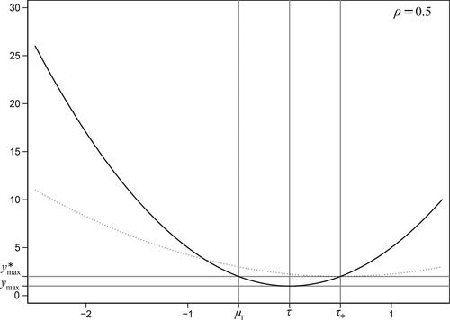
Let $y_{\max }\equiv \alpha +\beta \tau +\gamma {\tau }^2=\alpha -\gamma {\tau }^2$ be the minimum ($\gamma >0$) or maximum ($\gamma <0$) value of $\mathbb{E}(y|\xi ).$ With measurement error, its estimated counterpart converges to $y_{\max }^{*}=\alpha +\gamma ({\rho }^2{\tau }_{*}^2-{\tau }^2)+\pi -{\rho }^2\gamma {\tau }_{*}^2=y_{\max }+(1-\rho )\gamma {\sigma }_{\xi }^2.$ The results are depicted in Figure 1. The attenuation effect, well-known from the linear errors-in-variables model, shows up in the quadratic model in two forms. First, the graph has less curvature. Second, the minimal value is higher (lower if $\gamma <0$). Another effect is that the value of ξ where the minimum is attained is pushed away from its true value, but this can be in either direction depending on the position of τ relative to μ₁. These attenuation effects emphasize the importance of controlling for measurement error in the quadratic errors-in-variables model.

Figure 1. The effect of measurement error on the OLS-estimated curve.

Notes: The solid curve indicates the true relation, while the dotted curve reflects the estimated relation.

3. Method-of-moments estimation

This section focuses on the quadratic regression model with measurement error given by (1). We derive our method-of-moments estimator, discuss its identification and provide an extension to additional error-free control variables. Throughout, we maintain the assumptions that ξ, ε and v are mutually independent and that both the regression error ε and the measurement error v have mean zero and variances ${\sigma }_{\epsilon }^2$ and ${\sigma }_v^2,$ respectively. The only distributional assumption that we make is that v is symmetrically distributed and free of excess kurtosis, for which normality is a sufficient but not a necessary condition. Hence, in contrast to Section 2, we no longer impose any distributional assumptions on ξ.

3.1. Global outline of the approach

Our approach is to harvest enough moment conditions for consistent estimation. There are two first moments of y and x, three second moments, four third moments. If we use moments up to order k, their number adds up to $2+3+4+\cdots +(k+1)=k(k+3)/2.$ The expectation of the first k moments of y and x involves the parameters μ_j, $j=1,\dots ,2k.$ For v and ε, the number of moments is k − 1 each, since $\mathbb{E}(v)=\mathbb{E}(\epsilon )=0.$ There are three other parameters, namely α, β and γ. Hence, without assuming normality of any of the random terms, there are $4k+1$ parameters in total and a necessary condition for identification is $k(k+3)/2\ge 4k+1$ or $k^2-5k-2\ge 0.$ Hence, if we do not impose any further structure on the distribution of v, we need moments of at least order six. Estimators using such higher-order moments are expected to be sensitive to outliers, because the impact of extreme values on sample means is amplified by raising these large values to a high power. Under symmetry and zero excess kurtosis, the moments of v are fully determined by ${\sigma }_v^2.$ As a result, the parameters of the quadratic measurement-error model are identifiable from the first four moments of y and x.

The price we pay for the assumptions we impose on v is the risk of misspecification. Later we will therefore develop a statistical test to verify a necessary condition for the consistency of our method-of-moments estimator. This test is based on an auxiliary method-of-moments estimator that is consistent under symmetric measurement error, which requires moments up to order five.

3.2. Method-of-moments estimation

We formulate the following set of assumptions:

Assumptions 3.1.

1. We observe y and x, which come from the quadratic measurement-error model in (1).

2. ξ, ε and v are mutually independent with $\mathbb{E}(\epsilon )=\mathbb{E}(v)=0,\mathbb{E}({\epsilon }^2)={\sigma }_{\epsilon }^2$ and $\mathbb{E}(v^2)={\sigma }_v^2.$

3. v is symmetric. More specifically, (a) $\mathbb{E}(v^3)=0$ and (b) $\mathbb{E}(v^5)=0.$

4. v is free of excess kurtosis; i.e., ${\kappa }_v=\mathbb{E}(v^4)/{\sigma }_v^4=3.$

We note that the assumption of mutual independence of $\xi ,v$ and ε is in line with, e.g., Schennach and Hu (2013). We impose this assumption to ensure that the expectations of certain products of random variables reduce to the products of the expectations. The same effect could be achieved by imposing less stringent covariance assumptions of the form $\mathbb{C}\text{ov} (x_1^k,x_2^{\mathcal{\ell }})=0,$ for appropriate values of k and $\mathcal{\ell }$ and with $x_1,x_2\in \{v,\epsilon ,\xi \},x_1\cancel{=}{x}_2.$

Under Assumptions 3.1(i) – (iii), we find (8) $$\mathbb{E}(x)={\mu }_1$$(8) (9) $$\mathbb{E}(x^2)={\mu }_2+{\sigma }_v^2$$(9) (10) $$\mathbb{E}(x^3)=3{\mu }_1{\sigma }_v^2+{\mu }_3$$(10) (11) $$\mathbb{E}(x^4)=\mathbb{E}({\xi }^4+6{\xi }^2{v}^2+v^4)=6{\mu }_2{\sigma }_v^2+{\mu }_4+{\kappa }_v{\sigma }_v^4$$(11) (12) $$\mathbb{E}(x^5)=\mathbb{E}({\xi }^5+10{\xi }^3{v}^2+5\xi v^4)={\mu }_5+10{\mu }_3{\sigma }_v^2+5{\mu }_1{\kappa }_v{\sigma }_v^4,$$(12) where ${\kappa }_v\equiv \mathbb{E}(v^4)/{\sigma }_v^4$ denotes the kurtosis of v. Moment conditions (8) – (12) use $\mathbb{E}(v)=0,$ while (10) and (11) also use $\mathbb{E}(v^3)=0$ (i.e., Assumption 3.1 (iii-a)). Moment condition (12) additionally uses $\mathbb{E}(v^5)=0$ (i.e., Assumption 3.1 (iii-b)).

With ${\pi }_v\equiv (6-{\kappa }_v){\sigma }_v^4,$ we can rewrite (13) $$\left(\begin{array}{c}{\mu }_1\\ {\mu }_2\\ {\mu }_3\\ {\mu }_4\\ {\mu }_5\end{array}\right)=\mathbb{E}\left(\begin{array}{c}{m}_1\\ m_2\\ m_3\\ m_4\\ m_5\end{array}\right)\equiv \mathbb{E}\left(\begin{array}{c}x\hfill \\ x^2-{\sigma }_v^2\hfill \\ x^3-3{\sigma }_v^{2}x\hfill \\ x^4-6{\sigma }_v^2{x}^2+(6-{\kappa }_v){\sigma }_v^4\hfill \\ x^5-10{\sigma }_v^2{x}^3+5(6-{\kappa }_v){\sigma }_v^{4}x\hfill \end{array}\right)=\mathbb{E}\left(\begin{array}{c}x\hfill \\ x^2-{\sigma }_v^2\hfill \\ x^3-3{\sigma }_v^{2}x\hfill \\ x^4-6{\sigma }_v^2{x}^2+{\pi }_v\hfill \\ x^5-10{\sigma }_v^2{x}^3+5{\pi }_{v}x\hfill \end{array}\right).$$(13)

If we now also impose Assumption 3.1 (iv), we get ${\pi }_v=3{\sigma }_v^4.$ Then m₄ and m₅ in (13) reduce to $m_4=x^4-6{\sigma }_v^2{x}^2+3{\sigma }_v^4$ and $m_5=x^5-10{\sigma }_v^2{x}^3+15{\sigma }_v^{4}x.$ The parameters of interest are α, β, γ, ${\sigma }_{\epsilon }^2,{\sigma }_v^2,$ while the μ_ks are the nuisance parameters.

To estimate these parameters, we consider moment conditions involving moments up to order four, of which there are $2+3+4+5=14.$ We discard $\mathbb{E}(x{y}^3)$ and $\mathbb{E}(y^4),$ because they involve μ₇ and μ₈. We also ignore $\mathbb{E}(y^3)$ and $\mathbb{E}(x^2{y}^2),$ because they depend on μ₆. Theoretically, dropping moments and parameters may entail a slight loss of efficiency in estimating the other parameters. We nevertheless believe that this effect will be small relative to the advantage of not using unstable higher-order moments.

We thus consider the moments $\mathbb{E}(y),\mathbb{E}(xy),\mathbb{E}(x^{2}y),\mathbb{E}(x^{3}y),\mathbb{E}(y^2)$ and $\mathbb{E}(x{y}^2).$ Elimination of α by centering the variables is not straightforward in a quadratic model, so we keep the intercept and refrain from centering. We equivalently consider the moments of $\overline{y}\equiv y-\alpha$ instead of y and of the m_ks instead of the powers of x. We write m₁ for x for the sake of transparency. The moment conditions linear in $\overline{y}$ that we exploit are (14) $$\mathbb{E}(\overline{y})=\beta {\mu }_1+\gamma {\mu }_2$$(14) (15) $$\mathbb{E}(m_1\overline{y})=\mathbb{E}[(\xi +v)(\beta \xi +\gamma {\xi }^2)]=\beta {\mu }_2+\gamma {\mu }_3$$(15) (16) $$\mathbb{E}(m_2\overline{y})=\mathbb{E}[({\xi }^2+v^2-{\sigma }_v^2)(\beta \xi +\gamma {\xi }^2)]=\beta {\mu }_3+\gamma {\mu }_4$$(16) (17) $$\mathbb{E}(m_3\overline{y})=\mathbb{E}[({\xi }^3+3\xi v^2-3{\sigma }_v^2\xi )(\beta \xi +\gamma {\xi }^2)]=\beta {\mu }_4+\gamma {\mu }_5.$$(17)

After eliminating the μ_ks, this yields (18) $$\mathbb{E}(m_j\overline{y}-\beta m_{j+1}-\gamma m_{j+2})=0,$$(18) for $j=0,1,2,3$ and with $m_0\equiv 1.$ The moment conditions quadratic in $\overline{y}$ that we consider are $$\begin{array}{c}\mathbb{E}({\overline{y}}^2)=\mathbb{E}\left[{(\beta \xi +\gamma {\xi }^2+\epsilon )}^2\right]={\beta }^2{\mu }_2+2\beta \gamma {\mu }_3+{\gamma }^2{\mu }_4+{\sigma }_{\epsilon }^2=\mathbb{E}[(\beta m_1+\gamma m_2)\overline{y}]+{\sigma }_{\epsilon }^2\\ \mathbb{E}(m_1{\overline{y}}^2)=\mathbb{E}\left[\xi {(\beta \xi +\gamma {\xi }^2+\epsilon )}^2\right]={\beta }^2{\mu }_3+2\beta \gamma {\mu }_4+{\gamma }^2{\mu }_5+{\mu }_1{\sigma }_{\epsilon }^2=\mathbb{E}[(\beta m_2+\gamma m_3)\overline{y}]+{\mu }_1{\sigma }_{\epsilon }^2.\end{array}$$

After eliminating the μs, we find (19) $$\mathbb{E}({\overline{y}}^2-(\beta m_1+\gamma m_2)\overline{y}-{\sigma }_{\epsilon }^2)=0$$(19) (20) $$\mathbb{E}(m_1{\overline{y}}^2-(\beta m_2+\gamma m_3)\overline{y}-{\sigma }_{\epsilon }^2{m}_1)=0.$$(20)

Because (18) with j = 3 involves μ₅, we drop this condition. We then collect (18) [j = 0, 1, 2], (19) and (20) and write the system of moment equations as $\mathbb{E}[{\mathbf{h}}_1(\mathit{\theta };\mathbf{d})]=\mathbf{0},$ where $\mathbf{d}\equiv (x,y)\prime ,\mathit{\theta }\equiv (\alpha ,\beta ,\gamma ,{\sigma }_{\epsilon }^2,{\sigma }_v^2)\prime$ and (21) $${\mathbf{h}}_1(\mathit{\theta };\mathbf{d})\equiv \left(\begin{array}{c}\overline{y}-\beta m_1-\gamma m_2\\ m_1\overline{y}-\beta m_2-\gamma m_3\\ m_2\overline{y}-\beta m_3-\gamma m_4\\ {\overline{y}}^2-(\beta m_1+\gamma m_2)\overline{y}-{\sigma }_{\epsilon }^2\\ m_1{\overline{y}}^2-(\beta m_2+\gamma m_3)\overline{y}-{\sigma }_{\epsilon }^2{m}_1\end{array}\right).$$(21)

The method-of-moments estimator solves (22) $$\frac{1}{n}\sum _{i=1}^n{\mathbf{h}}_1(\mathit{\theta };{\mathbf{d}}_i)=\mathbf{0}.$$(22)

The resulting estimator $\widehat{\mathit{\theta }}$ will henceforth be referred to as “MM1” and its components are denoted by $\widehat{\alpha },\widehat{\beta },\widehat{\gamma },$ …. It uses Assumptions 3.1 (i), (ii), (iii-a) and (iv).

Alternatively, we can relax the assumption of no excess kurtosis and only assume symmetry of v. If we drop Assumption 3.1 (iv), the expectations of m₄ and m₅ in (13) contain ${\pi }_v=(6-{\kappa }_v){\sigma }_v^4.$ We therefore have to estimate the extended parameter vector $\mathit{\eta }\equiv (\alpha ,\beta ,\gamma ,{\sigma }_{\epsilon }^2,{\pi }_v,{\sigma }_v^2)\prime .$ We note that we estimate π_v instead of the kurtosis κ_v, because the underlying parameter transformation turned out to make it easier to find a numerical solution to the system of moment conditions.

Because of the additional parameter π_v, we add (18) with j = 3 to the moment conditions we already used for MM1. We collect (18) [$j=0,1,2,3$], (19) and (20) and write the system of moment conditions as $\mathbb{E}[{\mathbf{h}}_2(\mathit{\eta };\mathbf{d})]=\mathbf{0}.$ Our second method-of-moments estimator $\tilde{\mathit{\eta }},$ referred to as “MM2”, solves (23) $$\frac{1}{n}\sum _{i=1}^n{\mathbf{h}}_2(\mathit{\eta };{\mathbf{d}}_i)=\mathbf{0}.$$(23)

This estimator uses Assumptions 3.1 (i), (ii), (iii-a) and (iii-b). The components of $\tilde{\mathit{\eta }}$ will be denoted by $\tilde{\alpha },\tilde{\beta },\tilde{\gamma },$ ….

3.3. Asymptotic covariance matrix and identification

The method of moments is known to yield consistent and asymptotically normal estimators. To obtain the asymptotic covariance matrix corresponding to MM1, we need the Jacobian of the moment conditions with respect to the parameters as a function of the observed data. To obtain this matrix, we note that $\partial m_2/\partial {\sigma }_v^2=-1,\partial m_3/\partial {\sigma }_v^2=-3m_1,\partial m_4/\partial {\sigma }_v^2=-6m_2$ and $\partial \overline{y}/\partial \alpha =-1.$ The Jacobian writes as $${\mathbf{G}}_1(\mathit{\theta };\mathbf{d})=-\left(\begin{array}{ccccc}1& m_1& m_2& 0& -\gamma \\ m_1& m_2& m_3& 0& -(\beta +3\gamma m_1)\\ m_2& m_3& m_4& 0& \overline{y}-3\beta m_1-6\gamma m_2\\ 2\overline{y}-\beta m_1-\gamma m_2& \overline{y}{m}_1& \overline{y}{m}_2& 1& -\gamma \overline{y}\\ 2\overline{y}{m}_1-\beta m_2-\gamma m_3& \overline{y}{m}_2& \overline{y}{m}_3& m_1& -(\beta +3\gamma m_1)\overline{y}\end{array}\right).$$

With observed data ${\mathbf{d}}_1,\dots ,{\mathbf{d}}_n,$ this yields (24) $$\widehat{\mathbb{V}\text{ar}}(\widehat{\mathit{\theta }})=\frac{1}{n}{\left(\frac{1}{n}\sum _{i=1}^n{\mathbf{G}}_1(\widehat{\mathit{\theta }};{\mathbf{d}}_i)\right)}^{-1}\left(\frac{1}{n}\sum _{i=1}^n{\mathbf{h}}_1(\widehat{\mathit{\theta }};{\mathbf{d}}_i){\mathbf{h}}_1(\widehat{\mathit{\theta }};{\mathbf{d}}_i)\prime \right){\left(\frac{1}{n}\sum _{i=1}^n{\mathbf{G}}_1(\widehat{\mathit{\theta }};{\mathbf{d}}_i)\prime \right)}^{-1}.$$(24)

The model parameters are (locally) identified if the expectation of the Jacobian has full rank. This yields our main identification result.

Result 3.1. Under Assumptions 3.1 (i), (ii), (iii-a) and (iv), $\mathbb{E}({\mathbf{G}}_1(\mathit{\theta };\mathbf{d}))$ corresponding to MM1 fails to have full rank if γ = 0 or if ${\mu }_1={\mu }_2={\mu }_3=\beta =0.$ In the latter case, ξ = 0 with probability 1. This is a trivial case that we assume not applicable. As to the former:

1. If γ = 0, then γ is always identified.

2. If γ = 0 and β = 0, then all parameters except ${\sigma }_v^2$ are identified.

3. If γ = 0 and the skewness of ξ is 0, then only γ is identified.

4. In all other cases, all parameters are identified.

The proof of this result is in (online) Appendix A, supplementary material where we derive an explicit expression for the expectation of the Jacobian.

In finite samples and under misspecification, it is an empirical matter whether (22) has a unique solution $\widehat{\mathit{\theta }}$ that satisfies the feasibility conditions ${\widehat{\sigma }}_{\epsilon }^2\ge 0$ and $0\le {\widehat{\sigma }}_v^2\le {\widehat{\sigma }}_x^2,$ with ${\widehat{\sigma }}_x^2$ the sample variance of x. We will come back to the existence, uniqueness and feasibility of the solution in our simulation study in Section 6.

Similarly, we find that, under Assumptions 3.1 (i), (ii), (iii-a) and (iii-b), $\mathbb{E}({\mathbf{G}}_2(\mathit{\eta };\mathbf{d}))$ corresponding to MM2 fails to have full rank if either ${\mu }_1={\mu }_3=\beta =0$ or γ = 0. This is shown in Appendix A, supplementary material, where we derive an explicit expression for the expectation of the Jacobian. Again the existence, uniqueness and feasibility of a solution of (23) is an empirical matter in finite samples and under misspecification. Feasibility means that ${\tilde{\sigma }}_{\epsilon }^2\ge 0,0\le {\tilde{\sigma }}_v^2\le {\widehat{\sigma }}_x^2$ and ${\tilde{\pi }}_v\le 6{\tilde{\sigma }}_v^4,$ where the latter restriction follows from the non-negativity of the kurtosis. We will come back to this issue in our simulation study.

3.4. Error-free control variables

With an additional vector of error-free control variables $\mathbf{z}\in R^K,$ (1) becomes (25) $$y=\alpha +\beta \xi +\gamma {\xi }^2+\mathbf{z}\prime \mathit{\lambda }+\epsilon .$$(25)

For this extended model, consider the additional assumption that $(\xi ,\mathbf{z})$ is independent of both v and ε. We will refer to this as Assumption 3.1 (v).² This assumption yields the moment conditions (26) $$\mathbb{E}[\mathbf{z}(\overline{y}-\beta m_1-\gamma m_2)]=\mathbb{E}[\mathbf{z}(\epsilon -\beta v-\gamma (2\xi v+v^2-{\sigma }_v^2))]=\mathbf{0}.$$(26)

The inclusion of additional error-free regressors is straightforward: redefine $\overline{y}=y-\alpha -\mathbf{z}\prime \mathit{\lambda }$ in the moment conditions, add (26) to the moment conditions of either MM1 or MM2 and solve the resulting system of moment equations.

4. Statistical test

This section proposes a statistical test to validate a necessary assumption for the consistency of MM1 and discusses its statistical properties.

4.1. Diagnostic testing in the errors-in-variables model

With only observed covariates, the econometric literature provides an extensive array of tools for diagnostic and goodness-of-fit testing of regression models. For example, if we used specific-to-general model selection, we would typically first estimate an unrestricted model and perform some diagnostic and goodness-of-fit tests. Depending on the outcomes of these tests, we would subsequently revise the model by strengthening certain assumptions and by estimating an adjusted, more parsimonious regression model using a more efficient estimator. We would iteratively repeat these steps until the diagnostic tests indicated that the model assumptions cannot be strengthened any further, given the data under consideration.

In the presence of an error-ridden variable, however, such an approach is usually not possible. A major issue is that we observe neither the unobserved regressor nor the measurement error, making it impossible to apply tests to them. Simply ignoring the presence of measurement error is not an option either, since conventional statistical tests typically do not have the usual asymptotic properties in the presence of measurement error. Tailor-made diagnostic testing and variable selection for the errors-in-variables model is still in an early stage (Blalock, 1965; Bloch, 1978; Carrillo-Gamboa and Gunst, 1992; Huang et al., 2005; Huang and Zhang, 2013; Nghiem and Potgieter, 2019; Zhao et al., 2020).

An additional complication is that changing a single assumption of the errors-in-variables model already requires substantial changes in the underlying estimation method to maintain consistency. This form of ill-conditionedness of the errors-in-variables model explains why many estimators for this model rely on the standard assumption that the unobserved regressor, measurement error and regression error are mutually independent. We follow this convention by maintaining the usual independence assumptions, but we propose a statistical test to verify a necessary condition for the consistency of MM1.

4.2. Test statistic

Let ${\pi }_{v,2}={\text{plim}}_{n\to \infty }{\tilde{\pi }}_v$ and ${\sigma }_{v,2}^4={\text{plim}}_{n\to \infty }{({\tilde{\sigma }}_v^2)}^2.$ The restriction that we will test is ${\pi }_{v,2}=3{\sigma }_{v,2}^4.$ This property holds if v is symmetric and free of excess kurtosis, since MM2 is consistent in this case. We therefore use MM2 to construct a Wald test for testing the null hypothesis $H_0:{\pi }_v=3{\sigma }_v^4$ against the alternative hypothesis $H_1:{\pi }_v\cancel{=}3{\sigma }_v^4.$ This yields the test statistic (27) $$q_{\mathrm{W}}={\{{\tilde{\pi }}_v-3{({\tilde{\sigma }}_v^2)}^2\}}^2{\left(R\prime \widehat{\mathbb{V}\text{ar}}(\tilde{\mathit{\eta }})R\right)}^{-1},$$(27) where $R=(0,0,0,0,1,-6{\tilde{\sigma }}_v^2)\prime .$ We reject the null hypothesis at the $u\%$ significance level if $q_{\mathrm{W}}>{\chi }_{1,1-u}^2;$ otherwise do not reject.

To investigate the asymptotic size and power of the Wald test, we first discuss a few special cases. Under the null hypothesis that v has a symmetric distribution without excess kurtosis, MM2 is consistent such that ${\pi }_{v,2}=3{\sigma }_{v,2}^4.$ As a result, $q_{\mathrm{W}}$ is asymptotically ${\chi }_1^2$ distributed, yielding an asymptotic rejection rate (size) of u. For symmetric alternatives with ${\pi }_v\cancel{=}3{\sigma }_v^4,$ MM2 is still consistent. Consequently, we must have ${\pi }_{v,2}\cancel{=}3{\sigma }_{v,2}^4,$ yielding an asymptotic rejection rate (power) of 1. Because both MM1 and MM2 assume a symmetric measurement-error distribution, we cannot construct a test for the symmetry assumption on the basis of these two estimators. For asymmetric alternatives, nevertheless, our Wald test will have an asymptotic rejection rate of 1 as long as ${\pi }_{v,2}\cancel{=}3{\sigma }_{v,2}^4$ (Cameron and Trivedi, 2005, Ch. 7). Hence, as long as the inconsistency of MM2 causes ${\pi }_{v,2}$ to be different from $3{\sigma }_{v,2}^4,$ the asymptotic power of the Wald test will be 1 for asymmetric alternatives.

We will investigate the finite-sample behavior of MM2 and the Wald test by means of a simulation study in Section 6, where we will consider both symmetric and asymmetric alternatives.

5. Benchmark approach

Before discussing the results of a simulation study, we explain the approach of Schennach and Hu (2013). This approach will be used as a benchmark approach in our simulation study, together with OLS.

5.1. Sieve-based estimation

The semi-parametric estimator of Schennach and Hu (2013) applies to general non-linear models of the form $y=g(\xi ,\mathit{\tau })+\epsilon ,$ with $g(·,·)$ a parametric function of the unobserved regressor and a finite-dimensional parameter vector $\mathit{\tau }.$ The joint density of the observables (y, x) is denoted by f_yx. This joint density depends on the marginal densities of the regression error (f₁), the measurement error (f₂) and the unobserved regressor (f₃) via the following integral equation: (28) $$f_{yx}(y,x)=\int f_1(y-g(\xi ,\mathit{\tau }))f_2(x-\xi )f_3(\xi )d\xi .$$(28)

Schennach and Hu (2013) provide the conditions under which this equation is non-parametrically identified and thus yields a unique functional solution $(\mathit{\tau },f_1,f_2,f_3).$

Schennach and Hu (2013) propose a sieve-based approach using maximum-likelihood estimation. Thanks to the use of sieve densities, their approach does not require distributional assumptions such as symmetry of the measurement error. The method involves maximum likelihood estimation subject to non-linear parameter constraints. Applied to our quadratic specification, the log-likelihood function is given by (29) $$L\equiv \sum _{i=1}^n\hspace{0.17em}\text{log}\hspace{0.17em}\int f_1^{*}(y_i-\alpha -\beta \xi -\gamma {\xi }^2)f_2^{*}(x_i-\xi )f_3^{*}(\xi )d\xi .$$(29)

The densities $f_1^{*},f_2^{*}$ and $f_3^{*}$ are chosen to be sieve densities of the form (30) $$f_k^{*}(z)={(\sum _{j=0}^{s_k}{\delta }_j^k{p}_j(z))}^2\mathrm{\hspace{1em}}\mathrm{\hspace{1em}}[k=1,2,3],$$(30) for unknown coefficients ${\delta }_0^k,\dots ,{\delta }_{s_k}^k$ and sieve smoothing parameters s_k. The functions $p_j(z)$ are orthonormal Hermite polynomials, with $p_j(z)=(1/\sqrt{\pi }j!2^j)H_j(z)\hspace{0.17em}\text{exp}\hspace{0.17em}(-z^2/2),H_0(z)=1,H_1(z)=2z$ and $H_{j+1}(z)=2z{H}_j(z)-2j{H}_{j-1}(z).$ Parameter constraints must be imposed to ensure that each of the three sieve densities integrate to unity and that the first two have mean zero: (31) $$\sum _{j=0}^{s_k}{({\delta }_j^k)}^2=1\hspace{1em}[k=1,2,3];\mathrm{\hspace{1em}}\mathrm{\hspace{1em}}\sum _{j=0}^{s_k-1}\sqrt{2(j+1)}{\delta }_j^k {\delta }_{j+1}^k=0\hspace{1em}[k=1,2].$$(31)

Because of these parameter restrictions, we must have $s_k\ge 2$ for k = 1, 2 and $s_3\ge 1$ to ensure that the resulting sieve densities have at least one free parameter left after the parameter conditions have been imposed.

Because ${\sigma }_{\epsilon }^2,{\sigma }_v^2,{\sigma }_{\xi }^2$ and μ₁ are all functions of the δs, the parameters in the parameter vector $\mathit{\tau }=({\delta }_0^1,\dots ,{\delta }_{s_1}^1,{\delta }_0^2,\dots ,{\delta }_{s_2}^2,{\delta }_0^3,\dots ,{\delta }_{s_3}^3,\alpha ,\beta ,\gamma )\prime$ are estimated jointly.

Schennach and Hu (2013) show that the sieve-based approach is $\sqrt{n}$-consistent for $s_k\to \infty$ as $n\to \infty ,$ k = 1, 2, 3. In practice, the values of the sieve smoothing parameters s₁, s₂ and s₃ will have to be chosen in a data-driven way, for example using a cross-validation approach that aims to minimize a mean squared error. Such an approach would be too time-consuming for our simulation study and is therefore omitted. Instead, we will use the same set of smoothing parameters across different sample sizes.

In an empirical application, Schennach and Hu (2013) obtain standard errors using a bootstrap procedure. Such a procedure would be again be too time-consuming for our simulation study. In line with Schennach and Hu (2013) and Garcia and Ma (2017), we will therefore not report standard errors for the sieve-based estimates.³

If the quadratic errors-in-variable model contains error-free control variables as in (25), we condition all densities in (28) and (29) on these covariates. Because of the assumed independence, the densities f₁ and f₂ are not affected by this conditioning. Regarding f₃, we adopt the two-step estimation approach proposed by Schennach and Hu (2013, p. 184). We first estimate $\mathbb{E}(\xi |\mathbf{z})$ by regressing x on a constant and the vector of control variables z, yielding the estimated coefficient vector $\widehat{\mathit{\zeta }}.$ Subsequently, we replace $f_3^{*}(\xi )$ in (29) by $f_3^{*}(\xi -\widehat{\mathit{\zeta }}\prime \mathbf{z})$ and $f_1^{*}(y_i-\alpha -\beta \xi -\gamma {\xi }^2)$ by $f_1^{*}(y_i-\alpha -\beta \xi -\gamma {\xi }^2-\mathbf{z}\prime \widehat{\mathit{\lambda }}).$ We then proceed as above, but with the additional constraint that the sieve density $f_3^{*}$ has mean zero.

5.2. Comparison to method of moments

Table 2 compares the assumptions underlying our method-of-moments estimator MM1 and the sieve-based estimator of Schennach and Hu (2013). Both estimators assume that ξ, v and ε are mutually independent. The main advantage of the method of Schennach and Hu (2013) lies in its flexibility with respect to the functional form of $g(\xi ,\mathit{\tau }),$ which does not have to be quadratic. The sieve-based approach is also relatively flexible with respect to the distribution of the measurement error, which is not required to be symmetric or free of excess kurtosis.

Table 2. Assumptions: method-of-moments vs. sieve-based estimation.

Assumption	Method of moments	Sieve based estimation
$\mathbb{E}(y|\xi ,\mathbf{z})$	quadratic	non-parametric (sieve)^a
regression error ε	none	non-parametric (sieve)^a
measurement error v	normal	non-parametric (sieve)^a
unobserved regressor ξ	none	non-parametric (sieve)^a
distribution of $\xi |\mathbf{z}$	none	restricted^b

^aIn practice, parametric with few terms, but more flexible than normal; see description in text.

^b$\mathbb{E}(\xi |z)$ is assumed linear and distribution of $\xi -\mathbb{E}(\xi |\mathbf{z})|\mathbf{z}$ assumed independent of z.

We note, however, that sieve densities will impose certain parametric restrictions in practice. This is due to the relatively low values of the numbers of terms s_k that are usually selected in (30) for the sake of computational feasibility. Such restrictions are particularly relevant for the distributions of ξ and ε, on which the method of moments does not impose any assumptions. Hence, the sieve-based method will typically be more general in terms of the distribution of v, but less general regarding the distributions of ξ and ε.

If a vector of error-free control variables z is included in the quadratic measurement-error model as in (25), both approaches assume that $(\xi ,\mathbf{z}),$ v and ε are mutually independent. The sieve-based approach additionally assumes that $\mathbb{E}(\xi |\mathbf{z})=\mathbf{z}\prime \mathit{\zeta }$ and that $[\xi -\mathbb{E}(\xi |\mathbf{z})]|\mathbf{z}$ does not depend on z. Our method-of-moments estimators do not require such assumptions.

6. Simulation study

We use Monte Carlo simulation to assess the performance of MM1, the Wald test, the sieve-based approach and OLS. In all simulation experiments, we take $n=500,2,000,3,000$ and $5,000.$

6.1. Normal measurement error

We start with the normal quadratic measurement-error model given by (1), with $\alpha =\beta =\gamma =1,\epsilon \sim \mathcal{N}(0,2),v\sim \mathcal{N}(0,0.2)$ and $\xi \sim \mathcal{N}(1,1).$ The model has an R² of 0.85 and a reliability of 0.83.⁴

Because the measurement error in our simulation experiment is normally distributed, MM1 is consistent. The sieve-based approach of Schennach and Hu (2013) is also consistent in this setting, provided that $s_k\to \infty$ as $n\to \infty ,$ k = 1, 2, 3. Because we use $s_1=s_2=s_3=6$ regardless of the sample size, the empirical implementation of the sieve-based estimator is formally inconsistent. Because of the flexibility of the sieve densities even for relatively low values of the smoothing parameters, we still expect the resulting estimator to perform well in terms of bias and standard deviation. However, we expect MM1 to have a smaller bias and to be more efficient, since it does not rely on approximative distributions but exploits the assumptions of symmetry and zero excess kurtosis.

The upper panel of Table 3 (“normal errors”) shows the results for MM1, the sieve-based approach and OLS. The rows captioned “bias” report the average value of the estimated parameter minus its true value. The rows captioned “s.d.” show the standard deviation of the estimated parameters, while the rows captioned “avg. $\widehat{\sigma }$” display the average estimated standard errors. These statistics are calculated as averages over all simulation runs for which the system of moment conditions has a unique solution. We verify the uniqueness of the solution by using different starting values for the root-solving routine. We confirm the existence of a unique solution in almost all simulation runs. Regardless of the sample size, the estimates of α, β, γ, ${\sigma }_{\epsilon }^2$ and ${\sigma }_v^2$ as produced by MM1 are on average close to their true values. Also the average formula-based standard errors are close to the sample standard deviations. Also for smaller sample sizes, MM1 usually turns out feasible.⁵

Table 3. Simulation results: normal errors.

	Method of moments (MM1)					Sieve based			OLS
	α	β	γ	${\sigma }_{\epsilon }^2$	${\sigma }_v^2$	α	β	γ	α	β	γ
Normal errors
$n=500$
bias	–14	–44	32	–63	–1	–90	92	15	359	107	–302
s.d.	149	217	143	448	40	134	203	100	105	124	65
avg. $\widehat{\sigma }$	143	205	128	417	39	n.a.	n.a.	n.a.	61	68	27
$n=2,000$
bias	–1	–6	4	–5	–1	–83	39	40	362	112	–306
s.d.	75	103	68	229	21	72	121	59	52	63	33
avg. $\widehat{\sigma }$	72	100	66	217	20	n.a.	n.a.	n.a.	30	33	13
$n=3,000$
bias	1	–3	2	–2	–1	–75	33	42	361	111	–305
s.d.	60	82	55	175	16	62	106	53	45	49	26
avg. $\widehat{\sigma }$	59	82	54	180	17	n.a.	n.a.	n.a.	25	27	11
$n=5,000$
bias	1	–1	0	2	–1	–41	56	7	362	111	–306
s.d.	45	65	44	145	14	78	95	84	33	39	22
avg. $\widehat{\sigma }$	46	63	42	140	13	n.a.	n.a.	n.a.	19	21	8
Discrete regression error
$n=500$
bias	–11	–29	22	–53	0	–178	110	94	2363	113	–307
s.d.	155	217	144	474	41	131	220	111	109	125	66
avg. $\widehat{\sigma }$	148	201	127	433	39	n.a.	n.a.	n.a.	61	68	27
$n=2,000$
bias	–1	–4	3	–5	–1	–123	53	73	2361	112	–306
s.d.	74	99	68	233	21	56	96	46	51	60	32
avg. $\widehat{\sigma }$	75	99	66	227	21	n.a.	n.a.	n.a.	30	33	13
$n=3,000$
bias	1	1	–1	0	–1	–131	64	79	2362	113	–307
s.d.	62	80	53	181	16	56	83	41	44	49	26
avg. $\widehat{\sigma }$	61	81	54	186	17	n.a.	n.a.	n.a.	25	27	11
$n=5,000$
bias	0	–1	1	–7	0	–121	56	78	2362	112	–306
s.d.	48	63	44	146	13	37	65	30	34	38	21
avg. $\widehat{\sigma }$	47	63	42	145	13	n.a.	n.a.	n.a.	19	21	8

Notes: The underlying measurement-error model is given by (1), with $\alpha =\beta =\gamma =1,{\sigma }_{\epsilon }^2=2$ and ${\sigma }_v^2=0.2.$ In the upper panel (“Normal errors”), the measurement and the regression error are normally distributed. In the lower panel (“Discrete regression error”), the measurement error is normal again but the regression error has a (demeaned) Poisson distribution. The sieve-based method uses $s_1=s_2=s_3=6.$ In this and subsequent tables, the rows captioned “bias” report the value of the estimated parameter minus its true value, averaged over the simulation runs. The rows captioned “s.d.” show the standard deviation of the estimated parameter over the simulations, while the rows captioned “avg. $\widehat{\sigma }$” displays the average estimated standard error over the simulations. All figures have been multiplied by 1,000 for easier comparison. The number of simulation runs is 1,000 (OLS and method of moments) and 100 (sieve-based method).

The biases of the sieve-based estimators are small in an absolute sense but larger than those associated with MM1. Part of this difference in bias may be caused by our non-optimal choice of the sieve smoothing parameters s_k. The biases of the sieve-based estimators of β and γ do not show the monotonic decrease with n that we may expect on the basis of the method’s known consistency. The pattern in the biases is also likely to reflect our fixed choice of smoothing parameters and emphasizes the need for a data-driven choice to get optimal results. As expected, the results in the upper panel of Table 3 confirm that the OLS estimator is inconsistent.

We also consider the above quadratic errors-in-variables model with (demeaned) Poisson distributed regression errors. We choose the same regression error variance as before, which means that we set the Poisson parameter equal to 2. Because MM1 does not use the distribution of ε, we do not expect that this distributional change will substantially affect its performance. By contrast, the ability of the sieve estimator with low s₁ to approximate the discrete distribution of ε could be affected. These expectations are confirmed by the results shown in the lower panel of Table 3. Especially the bias of the sieve-based estimator of α turns out relatively large for $s_1=s_2=s_3=6.$ The OLS bias continues to be large.

6.2. Non-normal measurement error

We take the same quadratic measurement error as before, but now with non-normal, symmetric measurement error. As before, we set $\alpha =\beta =\gamma =1,\epsilon \sim \mathcal{N}(0,2)$ and $\xi \sim \mathcal{N}(1,1),$ but choose v either Laplace distributed (leptokurtic) or continuous-uniformly distributed (platykurtic) with mean 0 and variance 0.2. Because zero excess kurtosis is a necessary condition for the consistency of MM1, this estimator will be inconsistent in these two cases. We expect the sieve-based estimator, based on $s_1=s_2=s_3=6,$ to be less inconsistent than MM1.

The estimation results are shown in upper and lower panel of Table 4. Regardless of the sample size, the biases of $\widehat{\alpha },\widehat{\beta }$ and $\widehat{\gamma }$ are less than 10% of the true parameter values. The biases of ${\widehat{\sigma }}_{\epsilon }^2$ and ${\widehat{\sigma }}_v^2$ are more substantial, though. The inconsistency of the underlying approach becomes apparent from the biases’ lack of variation with n. As expected, the biases of the sieve-based estimators are small in an absolute sense. In comparison to MM1, however, the biases of the sieve-based estimates of α and γ are relatively large. As before, the biases of the sieve-based estimators do not show the convergence to zero that would be the case with optimal smoothing parameters. As expected, the bias of the OLS estimator is much larger than for the other two methods.

Table 4. Simulation results: non-normal symmetric measurement error.

	Method of moments (MM1)					Sieve based			OLS
	α	β	γ	${\sigma }_{\epsilon }^2$	${\sigma }_v^2$	α	β	γ	α	β	γ
Laplace measurement error
$n=500$
bias	–84	58	31	–369	30	–129	94	39	366	156	–328
s.d.	223	342	175	724	70	120	263	116	112	146	86
avg. $\widehat{\sigma }$	186	272	149	595	60	n.a.	n.a.	n.a.	61	67	26
$n=2,000$
bias	–67	90	3	–299	30	–124	79	55	367	166	–333
s.d.	94	154	79	325	35	70	141	68	56	75	45
avg. $\widehat{\sigma }$	87	129	74	299	33	n.a.	n.a.	n.a.	30	33	13
$n=3,000$
bias	–68	92	3	–303	31	–92	68	37	366	167	–334
s.d.	73	112	64	267	29	67	144	60	47	60	36
avg. $\widehat{\sigma }$	72	107	62	251	27	n.a.	n.a.	n.a.	25	27	11
$n=5,000$
bias	–61	91	–1	–277	29	–86	63	37	367	165	–333
s.d.	55	87	49	191	21	59	131	56	36	47	28
avg. $\widehat{\sigma }$	54	81	48	191	21	n.a.	n.a.	n.a.	19	21	8
Uniform measurement error
$n=500$
bias	15	–72	24	54	–13	–126	67	51	359	84	–293
s.d.	146	206	141	440	36	116	257	118	103	121	61
avg. $\widehat{\sigma }$	139	192	125	395	34	n.a.	n.a.	n.a.	61	68	27
$n=2,000$
bias	22	–40	3	93	–12	–97	48	44	359	89	–295
s.d.	71	92	63	214	18	71	160	62	51	60	30
avg. $\widehat{\sigma }$	69	93	63	202	18	n.a.	n.a.	n.a.	30	34	13
$n=3,000$
bias	22	–42	4	94	–12	–94	40	48	358	87	–294
s.d.	58	78	53	176	16	63	119	54	42	50	24
avg. $\widehat{\sigma }$	57	76	52	167	15	n.a.	n.a.	n.a.	25	27	11
$n=5,000$
bias	25	–36	–1	105	–13	–100	57	42	360	88	–295
s.d.	44	62	41	126	11	55	117	52	32	39	19
avg. $\widehat{\sigma }$	44	59	40	131	11	n.a.	n.a.	n.a.	19	21	8

Notes: The underlying measurement-error model is given by (1), with normal regression error and $\alpha =\beta =\gamma =1,{\sigma }_{\epsilon }^2=2$ and ${\sigma }_v^2=0.2.$ In the upper panel (“Laplace measurement error”), the measurement error is Laplace distributed. In the lower panel (“Uniform measurement error”), the measurement error is uniformly distributed. The sieve-based method uses $s_1=s_2=s_3=6.$ Excess kurtosis: 3 (Laplace) and $-6/5$ (continuous uniform).

We also consider the quadratic measurement-error model with non-symmetric measurement error. We use the same specification as used by Schennach and Hu (2013) in their simulation experiments. We thus set α = 0, $\beta =\gamma =1$ and $\epsilon \sim \mathcal{N}(0,0.9).$ Furthermore, ξ is a mixture of $\mathcal{N}(0,1)$ and $\mathcal{N}(0.2,0.25)$ random variables with weights 0.6 and 0.4, respectively. We take v (demeaned) minimum-Gompertz distributed, with parameters $a=0.5772b$ and b = 1/2, where 0.5772 denotes the Euler-Mascheroni constant. Due to the substantial measurement-error variance of about 0.4, the reliability in this model is lower than in the previously considered normal model (0.64 versus 0.83). The model’s R² is also lower than before and equals almost 0.70. Again we expect the sieve-based estimator, based on $s_1=s_2=s_3=5,$ to be less inconsistent than MM1.

The estimation results are shown in upper panel of Table 5 (“Gompertz measurement error”). We observe that MM1 is more biased than in the previous simulation experiments. This holds particularly true for the estimators of γ and ${\sigma }_v^2.$ The increased bias is due to the combination of a leptokurtic, asymmetric measurement-error distribution and a reduced reliability.

Table 5. Simulation results: Gompertz errors.

	Method of moments (MM1)					Sieve based			OLS
	α	β	γ	${\sigma }_{\epsilon }^2$	${\sigma }_v^2$	α	β	γ	α	β	γ
Gompertz measurement error
$n=500$
bias	12	91	–187	189	–164	–34	–11	81	181	–272	–503
s.d.	130	286	194	387	121	100	156	154	84	79	70
avg. $\widehat{\sigma }$	122	246	170	335	101	n.a.	n.a.	n.a.	54	43	26
$n=2,000$
bias	29	96	–206	214	–144	–35	–15	86	187	–267	–512
s.d.	64	141	86	176	55	52	84	83	46	39	39
avg. $\widehat{\sigma }$	60	127	82	164	48	n.a.	n.a.	n.a.	27	21	13
$n=3,000$
bias	31	87	–213	228	–147	–38	12	121	187	–263	–512
s.d.	50	111	68	141	44	41	62	76	36	31	31
avg. $\widehat{\sigma }$	48	102	66	133	39	n.a.	n.a.	n.a.	22	17	10
$n=5,000$
bias	32	90	–211	226	–144	–37	9	101	188	–264	–514
s.d.	39	84	53	108	33	34	52	56	29	25	25
avg. $\widehat{\sigma }$	38	80	52	104	31	n.a.	n.a.	n.a.	17	13	8
Gompertz errors
$n=500$
bias	19	88	–200	210	–180	–55	–26	65	181	–269	–508
s.d.	135	273	193	376	357	106	166	149	81	78	68
avg. $\widehat{\sigma }$	124	233	169	327	232	n.a.	n.a.	n.a.	54	43	26
$n=2,000$
bias	31	86	–212	221	–150	–46	–3	64	188	–264	–513
s.d.	61	139	87	186	56	57	75	83	46	40	39
avg. $\widehat{\sigma }$	60	122	83	168	49	n.a.	n.a.	n.a.	27	21	13
$n=3,000$
bias	31	91	–210	225	–145	–46	9	74	189	–263	–513
s.d.	51	108	71	144	43	49	69	72	37	32	31
avg. $\widehat{\sigma }$	49	101	69	139	41	n.a.	n.a.	n.a.	22	17	10
$n=5,000$
bias	30	88	–211	228	–146	–41	1	63	188	–264	–513
s.d.	38	87	54	111	35	32	64	54	30	25	26
avg. $\widehat{\sigma }$	39	81	54	110	33	n.a.	n.a.	n.a.	17	13	8

Notes: The underlying measurement-error model is given by (1), with α = 0, $\beta =\gamma =1,{\sigma }_{\epsilon }^2=0.9$ and ${\sigma }_v^2=0.4.$ In the upper panel (“Gompertz measurement error”), the measurement error has a Gompertz distribution and the regression error is normal. In the lower panel (“Gompertz errors”), the measurement and the regression errors have a Gompertz distribution. The sieve-based method uses $s_1=s_2=s_3=5.$ Excess kurtosis Gompertz measurement-error distribution: 2.4.

We next consider the Gompertz measurement-error model with non-normal regression errors. The distribution of the regression errors is (demeaned) minimum-Gompertz, with parameters $a=0.5772b$ for b = 3/4, while the remaining distributions and parameters are the same as before. Because MM1 does not rely on the distribution of ε, we would not expect this distributional change to affect its bias. The results in the lower panel of Table 5 (“Gompertz errors”) confirm this. The ability of the sieve estimator with low s₁ to approximate the distribution of ε could be affected, as it did before when we considered Poisson regression error. However, this time we do not observe the latter effect for the sieve-based estimators; the results in the lower panel of Table 5 are very similar to those in the upper panel.

6.3. Error-free control variables

We consider two simulation experiments for the quadratic normal-measurement error models with a single error-free control variable z, such that $\mathbf{z}\prime \mathit{\lambda }$ in (25) reduces to λz. In both simulation experiments, Assumption 3.1 (v) is satisfied. In the first experiment, we take $\alpha =\beta =\gamma =\lambda =1,\epsilon \sim \mathcal{N}(0,2),v\sim \mathcal{N}(0,0.2),z\sim \mathcal{N}(0.5,0.5)$ and $\xi |z\sim \mathcal{N}(0.75z,0.75).$ In the second experiment, we choose $\alpha =\lambda =1,\beta =\gamma =0.5,\epsilon \sim \mathcal{N}(0,2),v\sim \mathcal{N}(0,0.2),\xi \sim \mathcal{N}(1,1)$ and $z|\xi \sim \mathcal{N}(\xi ,1),$ such that $\mathbb{E}(\xi |\mathbf{z})$ is non-linear. In both models, the R² and the reliability have a value of 0.83.

Because the functional form of $\mathbb{E}(\xi |\mathbf{z})$ does not matter for the consistency of MM1, we expect good results for MM1 in both experiments. For the sieve-based approach ($s_1=s_2=s_3=6$), the two-step approach described at the end of Section 5.1 will only be consistent in the first simulation experiment.

The estimation results in Table C2 of Appendix C, supplementary material confirm our expectations. In both simulation experiments, the biases of MM1 are small in an absolute sense and vanish as n increases. In the first simulation experiment, the biases of the sieve-based estimators are also small, but larger than those associated with MM1. In the second experiment, the biases of the sieve-based estimators are much larger, both in an absolute sense and relative to MM1. For values of n larger than 500, the bias of the sieve-based estimator of $\widehat{\beta }$ is even larger than for OLS.

6.4. Wald test

Before turning to the performance of the Wald test in previously considered simulation experiments, we globally discuss the behavior of the auxiliary estimator MM2 in the simulations. We first observe that the underlying system of moment equations does not always yield a feasible solution that satisfies ${\tilde{\sigma }}_{\epsilon }^2\ge 0,0\le {\tilde{\sigma }}_v^2\le {\widehat{\sigma }}_x^2$ and ${\tilde{\pi }}_v\le 6{\tilde{\sigma }}_v^4.$ Most of the time, infeasibility is caused by violation of the last constraint. In a small percentage of the simulation runs, there is no solution at all.⁶

Our simulation experiments confirm that MM2 is consistent, but show that it may turn out inefficient relative to MM1 if v is normal, depending on the coefficients of interest.⁷ Similarly, they confirm that if v is symmetric with non-zero excess kurtosis, MM2 is consistent, as opposed to MM1. In the asymmetric case, the relative performance of MM1 and MM2 is an empirical matter, since both estimators will usually be inconsistent. In the Gompertz case, our simulation results show that the biases of $\widehat{\alpha },\widehat{\beta }$ and $\widehat{\gamma }$ (MM1) are smaller than those of $\tilde{\alpha },\tilde{\beta }$ and $\tilde{\gamma }$ (MM2). However, MM2 produces a less biased estimate of ${\sigma }_v^2.$ As a possible explanation for this performance difference, we note that MM1 erroneously imposes ${\pi }_v=3{\sigma }_v^4$ (Assumption 3.1 (iv)) but does not assume $\mathbb{E}(v^5)=0$ (Assumption 3.1 (iii-b)), unlike MM2. Apparently, the former assumption is less detrimental to the consistent estimation of α, β and γ than the latter, while the opposite holds for ${\sigma }_v^2.$

Our approach consists of running the Wald test whenever MM1 and MM2 both uniquely exist. This is virtually always the case in our simulations.⁸ Table 6 reports the empirical rejection rates of our Wald test in each of the eight simulation experiments considered previously. In the four cases with normal measurement error, these rejection rates reflect the empirical size of the Wald test. We see that these rejection rates are close to nominal. The rejection rates for the other simulation experiments reflect the empirical power of the Wald test. With Laplace and uniform measurement error, the empirical power starts at a relatively low level and increases slowly with n. The low finite sample power arises from the fact that MM1’s bias is only small in the presence of symmetric measurement error with non-zero excess kurtosis and modest variance. Only moment condition (11) does not hold, which results in an estimator whose inconsistency is relatively modest. Because the bias of MM1 is only small in these symmetric cases, the low power of the test poses less of a practical problem here. In the two Gompertz cases, however, the inconsistency of MM1 is more severe. Here the Wald test’s empirical power is already high for n = 500 and reaches the value 1 quickly.

Table 6. Empirical size and power of Wald test.

n	500	2, 000	3, 000	5, 000
Normal errors	10.5	7.7	8.0	6.4
Discrete regression error	10.9	5.7	5.6	5.7
Error-free regressor ($\xi \to z$)	6.9	4.9	6.8	6.6
Error-free regressor ($z\to \xi$)	6.8	6.8	5.4	4.5
Laplace measurement error	7.6	7.8	10.7	20.5
Uniform measurement error	13.1	15.0	20.7	24.3
Gompertz measurement error	81.7	99.6	100.0	100.0
Gompertz errors	78.3	99.7	100.0	100.0

Notes: This table applies to all of the simulations experiments that we performed and reports the rejection rates (in %) for the Wald test. In the upper panel, the reported percentages represent the empirical size of the test. In the lower panel, the percentages reflect the empirical power.

6.5. Outlier sensitivity

Because the impact of extreme values on sample means is amplified by raising these large values to a power up and until order four (MM1) and five (MM2), our method-of-moments estimators could be sensitive to outliers. We investigate the outlier sensitivity by means of simulation. For this purpose, we return to the model of Section 6.1 with normal measurement-error and regression error. In this adjusted simulation experiment, both ξ and ε contain 25 randomly placed outliers. The fixed number of outliers implies that their presence becomes less of an issue as n grows, which seems a realistic setup. These outliers have a positive or negative sign with probability 0.5 and their fixed magnitude is $q{\sigma }_{\xi }^2$ and $q{\sigma }_{\epsilon }^2$ (q = 2, 4, 5), respectively. To save space, the simulation results for MM1 are shown in Table C3 of Appendix C, supplementary material.

MM1 still feasibly exists in most simulation runs, even for the smaller sample sizes. But we observe that the presence of outliers tends to increase the bias of the estimated coefficients. This holds true especially for ${\sigma }_{\epsilon }^2.$ Also the standard deviation and average formula-based standard error of ${\sigma }_{\epsilon }^2$ increase substantially due to the presence of outliers. This effect becomes particularly apparent for q = 4, 5 and n = 500.

The simulation results reveal similar outlier effects for MM2 as for MM1.⁹ However, the percentage of simulation runs in which MM2 feasibly exists is relatively low for q = 4, 5 and n = 500. For example, if we take q = 5 and n = 500, then MM2 uniquely (feasibly) exists in 83.0% (18.3%) of the simulation runs. Further inspection shows that it is usually MM2’s infeasibility of ${\sigma }_v^2$ that is a problem in these simulations. For MM1, the two percentages are both 99.1%. Hence, MM2 is more sensitive to outliers than MM1 in terms of feasibility. The simulation results in the Appendix, supplementary material additionally show that our Wald test exhibits more overrejection if the magnitude of the outliers increases.

We conclude that our method-of-moments approach requires us to remain alert for outliers, especially if the sample size is relatively small.

6.6. Empirical strategy

Under the assumption of Schennach and Hu (2013) that “measurement error is not sufficiently severe to completely alter the shape of the specification,” we recommend considering our method-of-moments estimator as a potential candidate if OLS reveals a quadratic relation. Based on our analysis and simulations, we propose the following strategy to determine if MM1 should be used. If both MM1 and MM2 exist and the Wald test fails to reject, we recommend MM1 as the estimator of the quadratic errors-in-variables model. If the Wald test rejects, we recommend the approach of Schennach and Hu (2013) instead. We also recommend the latter approach if either MM1 or MM2 does not exist. However, we advise to remain alert for possible misspecification in such cases, especially in the presence of error-free control variables z. That is, in the presence of such regressors, the method of Schennach and Hu (2013) imposes certain assumptions on the conditional distribution of ξ given z; see the discussion in Section 5.2. Our simulations in Section 6.3 have shown that imposing these assumptions may lead to serious bias if they do not hold.

7. Empirical application

Our empirical application uses housing data from Harrison and Rubinfeld (1978).¹⁰ This data set contains information on 506 geographical neighborhoods (census tracts) in the Boston Standard Metropolitan Statistical Area in 1970. The dependent variable of interest is the median value of the owner-occupied homes in the census tract. The average median value of the homes in the data set equals $22,523, with a standard deviation of $9,182.

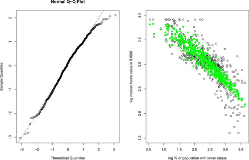
We assume that there is a single unobserved regressor of interest, namely the percentage of the population in the census tract with a lower socio-economic status. This percentage is measured as the equally-weighted average of the percentage of adults without some high-school education and the percentage of male workers classified as laborers. On average, the observed percentage of lower status population equals 12.7%, with a standard deviation of 7.1%. We informally investigate the normality of the log of the observed percentage of lower status population by drawing a QQ plot; see the first graph in Figure 2. The dashed line in this graph represents the 45 degree line, corresponding to the standard normal distribution. We observe some deviations from normality in the right tail, which is less heavy than in the normal case.

Figure 2. Boston housing data.

Notes: The QQ plot in the left-hand-side figure applies to the log of the observed percentage of lower status population (after standardization). The dashed line indicates the 45 degree line, corresponding to the standard normal distribution. In the right-hand-side figure, the open dots reflect the observed data, while the closed dots correspond to the OLS-based predicted (=expected) log housing value.

We consider the quadratic measurement-error model specified by (32) $$\text{log}\hspace{0.17em}(y)=\alpha +\beta \hspace{0.17em}\text{log}\hspace{0.17em}(\xi )+\gamma {[\text{log}\hspace{0.17em}(\xi )]}^2+\mathbf{z}\prime \mathit{\lambda }+\epsilon ;\mathrm{\hspace{1em}}\mathrm{\hspace{1em}}\hspace{0.17em}\text{log}\hspace{0.17em}(x)=\hspace{0.17em}\text{log}\hspace{0.17em}(\xi )+v,$$(32) where y is the median value of the owner-occupied homes in the census tract expressed in thousands of dollars, x the observed percentage of lower status population, ξ the true percentage of lower status population, v the measurement error and ε the regression error. The vector $\mathbf{z}=(z_1,z_2,z_3,z_4)\prime$ includes four additional explanatory variables that were also used by Wooldridge (2012): z₁ is the average number of rooms per house, z₂ the log of the nitric oxides concentration in parts per 10 million, z₃ the log of the weighted distance in miles to five Boston employment centers and z₄ the pupil-teacher ratio in the neighborhood. We assume these covariates to be free of measurement error. Detailed sample statistics for the dependent and explanatory variables are given in Table D1 of Appendix D, supplementary material.

We proceed as in Sections 3.4 and 4.2 to obtain the method-of-moments estimator MM1 under Assumptions 3.1 (i) – (v). Subsequently, we run the Wald test to verify the assumption of no excess kurtosis. To obtain the sieve-based estimator, we follow the two-step approach outlined in Section 5.1 and make the required assumptions about the distribution of $\text{log}\hspace{0.17em}(\xi )|\mathbf{z}.$

7.1. Benchmark approaches

As mentioned in the introduction, we maintain the assumption of Schennach and Hu (2013) that “measurement error is not sufficiently severe to completely alter the shape of the specification.” On the basis of OLS and the Bayesian Information Criterion (BIC), we conclude that we have to include $\text{log}\hspace{0.17em}(\xi )$ and ${[\text{log}\hspace{0.17em}(\xi )]}^2$ to parsimoniously capture the relation between $\text{log}\hspace{0.17em}(y)$ and $\text{log}\hspace{0.17em}(\xi )$ but that higher-order terms are not required.¹¹ We therefore continue with the model that has the lowest BIC value, which is the model with linear and quadratic terms, but no cubic terms. The corresponding OLS estimation results are shown in the left-most panel of Table 7.

Table 7. Estimation results for the Boston housing data.

	OLS				Sieve-based method				Method of moments (MM1)
	Coeff.	s.e.	5%	95%	Coeff.	s.e.	5%	95%	Coeff.	s.e.	5%	95%
Intercept	3.630	0.250	3.179	3.991	4.017	0.311	3.379	4.384	4.722	0.541	3.827	5.605
Log(Status)	0.069	0.119	–0.120	0.277	0.129	0.180	–0.125	0.465	0.896	0.281	0.441	1.386
Log(Status)^2	–0.111	0.028	–0.161	–0.067	–0.154	0.042	–0.230	–0.093	–0.404	0.067	–0.516	–0.300
Rooms	0.078	0.023	0.044	0.120	0.037	0.024	0.007	0.086	–0.113	0.046	–0.193	–0.044
Log(NOx)	–0.514	0.099	–0.678	–0.357	–0.350	0.112	–0.541	–0.167	–0.013	0.170	–0.297	0.253
Log(Dist)	–0.195	0.040	–0.264	–0.129	–0.193	0.044	–0.261	–0.120	–0.306	0.058	–0.403	–0.214
PT–ratio	–0.036	0.004	–0.042	–0.029	–0.032	0.005	–0.040	–0.025	–0.019	0.008	–0.031	–0.006
${\sigma }_{\epsilon }^2$									0.009	0.004	0.001	0.015
${\sigma }_v^2$									0.064	0.007	0.051	0.074
Reliability									0.824
Adj. R^2	0.745

Notes: The underlying quadratic measurement-error model is given by (32). For the sake of comparability, all standard errors (“s.e.”) and 5% and 95% quantiles are based on a standard bootstrap with replacement consisting of 1,000 runs. The reliability is calculated as $1-{\widehat{\sigma }}_v^2/{\widehat{\sigma }}_x^2.$ Covariates used: Log(Status) = log percentage of lower status population; Rooms = average number of rooms per house; Log(NOx) = log of nitric oxides concentration in parts per 10 million; Log(Dist) = log of weighted distance in miles to five Boston employment centers; PT-ratio = pupil-teacher ratio.

We observe that the OLS estimate of γ is significantly negative according to the 90% bootstrap-based confidence interval that is reported in Table 7. As a result, the estimated relation between the expected log housing value and the log percentage of lower status population is described by a parabola that opens downwards. For each observation, we display the OLS-based predicted log housing value in the second graph of Figure 2, together with a scatter plot of $\text{log}\hspace{0.17em}(x)$ and $\text{log}\hspace{0.17em}(y).$ The curve in Figure 2 shows that we expect lower log housing values for neighborhoods with a higher log percentage of lower status population.

We use the 5% and 95% sample quantile of x to determine a relevant range of values for ξ. For this range of values, we obtain the OLS-based elasticity of y with respect to ξ; i.e., the marginal effect of $\text{log}\hspace{0.17em}(\xi )$ on $\text{log}\hspace{0.17em}(y).$ We visualize these results in Figure 3 and observe that housing values are inelastic in all neighborhoods.

Figure 3. Comparison of different estimators.

Notes: For each method, the solid lines in the left-hand-side figure show the estimated elasticity of the housing value with respect to the percentage of lower status, plotted as a function of the log percentage of lower status. The dashed lines constitute the corresponding 90% pointwise confidence interval based on a bootstrap with replacement. The log percentage of lower status population is taken between the 5% and 95% quantile of the observed log percentage of lower status population. In the right-hand-side figure, the three methods are compared in terms of the predicted log housing value (in $1,000) as a function of the log percentage of lower status. Here, the additional control variables have been set at their sample medians.

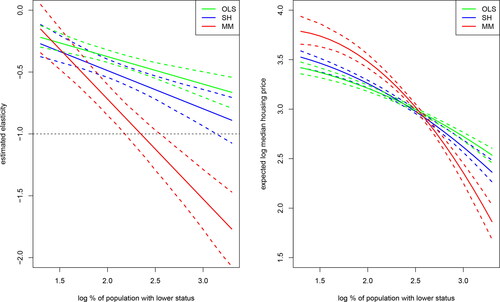
Subsequently, we estimate the quadratic measurement-error model using the sieve-based approach. In line with our simulation experiments, we use a trial-and-error procedure to determine the sieve smoothing parameters. This procedure entails that the values of the s_ks are increased until the resulting maximum likelihood estimates do not change any further, which yields the values $s_1=s_2=s_3=4.$ In line with Schennach and Hu (2013), we use a standard bootstrap with replacement to obtain the corresponding standard errors. The estimation results are shown in the middle panel of Table 7. According to the sieve-based method, the estimate of γ is significantly negative. We next calculate the estimated elasticity of y with respect to ξ and visualize the results in the first graph of Figure 3. We observe that housing values are either inelastic (low and medium percentage lower status) or unit elastic (very high percentage lower status).

According to both OLS and the sieve-based approach, the estimated coefficients of the additional control variables are significant and have the expected signs. However, on the basis of our simulation experiments, we note that some caution is required here. We seen that the bias of the OLS estimator can be substantial in the presence of measurement error. Furthermore, the sieve-based approach assumes that $\mathbb{E}(\hspace{0.17em}\text{log}\hspace{0.17em}(\xi )|\mathbf{z})=\mathbf{z}\prime \mathit{\zeta }$ and that $[\text{log}\hspace{0.17em}(\xi )-\mathbb{E}(\hspace{0.17em}\text{log}\hspace{0.17em}(\xi )|\mathbf{z})]|\mathbf{z}$ does not depend on z. Our simulation results have shown that erroneously imposing these assumptions may also induce substantial bias.

7.2. Method of moments

Lastly, we use MM1 to estimate the quadratic measurement-error model. The system of moment equations has a unique and feasible solution. Estimation results, including bootstrap-based standard errors, are reported in the right-most panel of Table 7. The estimate of γ is significantly negative. Furthermore, the estimate of the measurement-error variance is ${\widehat{\sigma }}_v^2=0.064,$ which translates into a reliability of 82%. Our empirical strategy recommends us to perform the Wald test, based on the auxiliary method-of-moments estimator. The latter estimator turns out to have a unique solution. We use a bootstrap-based version of the Wald test, which yields a p-value of 0.494. Hence, our test provides no evidence against the consistency of MM1.¹²

The first graph in Figure 3 visualizes the estimated elasticity of y with respect to ξ as a function of $\text{log}\hspace{0.17em}(\xi ),$ from which we conclude that housing values are inelastic (low percentage lower status), unit elastic (medium percentage lower status) or elastic (high percentage lower status). For medium to high percentages of the lower status population, the OLS-based elasticity curve lies significantly above the one based on MM1, in the sense that the former curve does not fall within the confidence bounds of the latter. The elasticity curve based on the sieve-based method falls in between the other two curves, but is relatively close to the OLS-based curve. The difference between the elasticity curves produced by OLS and MM1 is consistent with the effect of attenuation on the OLS estimates, as discussed in Section 2. To illustrate more directly that the graph based on MM1 has more curvature, the second graph in Figure 3 displays the predicted (=expected) value of $\text{log}\hspace{0.17em}(y)$ as a function of $\text{log}\hspace{0.17em}(\xi )$ for each of the three estimators.

According to MM1, the number of rooms has a significantly negative marginal effect, which seems counter-intuitive. We first investigate whether this finding is due to outliers, since our simulation results have shown that outlier sensitivity may be an issue for smaller sample sizes. We winsorize the dependent and explanatory variables at the 95% level and re-estimate the model. This adjustment leads to very little change in the sign, magnitude and significance of the estimated coefficients, suggesting that the counter-intuitive finding is not due to outliers.¹³ We provide two alternative explanations. First, Sirmans et al. (2005) and Zietz et al. (2008) address the insignificant or significantly negative coefficients of the number of (bed- or bath-)rooms that have shown up in certain studies. Zietz et al. (2008) argue that particular housing characteristics are priced differently for houses in the upper-price range as compared to houses in the lower-price range and recommend quantile regression to deal with this variation in pricing. Hence, the significantly negative sign of the coefficient estimate of the number of rooms may indicate that the standard quadratic location-shift regression model that we adopted is too restrictive. We refer to Chesher (2017) for a discussion of the effect of measurement error on the estimation of quantile regression functions. Consistent estimation of the quantile regression model in the presence of measurement error is also discussed in Schennach (2008) and Wei and Carroll (2009). We note, however, that these studies make use of side information in the form of instrumental variables and replicated measurements, respectively. A second possible explanation for the counter-intuitive sign is endogeneity due to simultaneity or omitted variables. Such a situation would require an approach that can deal with both measurement error and additional sources of endogeneity; see, e.g., Hu et al. (2015), Song et al. (2015) and Hu et al. (2016).

8. Discussion

This study has proposed a new consistent estimator for the quadratic errors-in-variables model, based on exploiting higher-order moment conditions. Our approach assumes a symmetric measurement-error (ME) distribution without excess kurtosis, but does not require any side information, such as a known measurement error variance, replicated measurements, or instrumental variables. We straightforwardly allow for one or more error-free control variables, which only requires the standard assumption that these regressors are independent of the measurement and regression errors. We have combined our estimator with a Wald-type statistical test to verify a necessary condition for its consistency.

Under the assumption that the measurement error does not alter the shape of the specification, we recommend considering our method-of-moments estimator as a potential candidate if OLS reveals a quadratic relation. On the basis of our theoretical analysis and simulation study, we recommend our estimator “MM1” as the final choice if the Wald test fails to reject. Especially if the sample size is small, we advise to investigate the sensitivity of the estimation results to outliers in the data.

We mention a few directions for future research. Instead of using our Wald test to choose between MM1 (symmetric ME with zero-excess kurtosis) and MM2 (symmetric ME), we may want to consider a different approach to obtain our final estimator. Because MM2 – unlike MM1 – is consistent even in the presence of excess kurtosis, an alternative possibility is to discard MM1 altogether and to resort to MM2 in all cases. Our simulation results have illustrated that this strategy does not necessarily lead to an estimator with a smaller bias or a lower variance, though. Furthermore, MM2 turned out relatively sensitive to outliers and small samples in terms of feasibility. Alternatively, we could resort to an approach that minimizes the final estimator’s Mean Squared Error (MSE). Methods such as shrinkage or model averaging could be used to strike an optimal balance between bias and variance. For a practical implementation of the latter approach, we refer to Lavancier and Rochet (2016). The latter study discusses a method to average different estimators of which at least one is consistent in order to reduce the MSE of the final estimator. We note that, in the absence of symmetry, both MM1 and MM2 will typically be inconsistent. As a result, the benefits of model-averaging remain theoretically unclear (Lavancier and Rochet, 2016). Preliminary estimation results in Lavancier and Rochet (2016) for a specific example show that the model-averaging approach is robust to model misspecification, but further research would be required to extrapolate this conclusion to our method-of-moment estimators.

The quadratic model is the natural first extension of the linear model, and arguably the most common extension used in practice. In principle, our approach could be extended to higher-order polynomials, but this would require fitting moments of a very high order, which would often lead to unacceptably large sampling variability. For other functional forms, it may be more natural to transform the error-ridden covariate first and assume additive measurement error on the transformed scale, similar to what we did in our empirical application.

We mention two other directions for future research. The first is the consistent estimation of the quantile regression model in the presence of measurement error and in the absence of any side information, as suggested by our empirical application. The second direction for future research is to relax the homoscedasticity implied by the independence assumption, which is often at variance with economic reality. We can extend our approach to handle heteroscedasticity, but only so at the cost of using moments of an order well beyond four. This requires enormous sample sizes and is hence not attractive. An alternative is to go back to earlier literature and express the heteroscedasticity as a parametric function of the regressors. In our case, this would involve the unobserved regressor, cf. Meijer and Mooijaart (1996) and Meijer (1998, Ch. 4). This option seems feasible, but our approach then evidently loses its relative simplicity. We emphasize, though, that this limitation is not unique to our approach (e.g., Garcia and Ma, 2017); heteroscedasticity remains a difficult issue to deal with and there is no simple escape by just using robust standard errors.

Acknowledgments

We thank participants of the 2018 Meeting of the Netherlands Econometric Study Group held at the University of Amsterdam for discussion and suggestions. We also thank Susanne Schennach and Yingyao Hu for discussions about their method and for sharing their Matlab code.

Laura Spierdijk gratefully acknowledges financial support from a Vidi grant (452.11.007) in the “Vernieuwingsimpuls” program of the Netherlands Organization for Scientific Research (NWO). Her work was also supported by the Netherlands Institute for Advanced Study in the Humanities and Social Sciences (NIAS-KNAW). The usual disclaimer applies.

Disclosure statement

No potential conflict of interest was reported by the authors.

Correction Statement

This article has been republished with minor changes. These changes do not impact the academic content of the article.

Notes

1 See also Chan and Mak (1985), Moon and Gunst (1995), Wolter and Fuller (1982), Buonaccorsi (1996), Cheng and Schneeweiss (1998), Cheng and Van Ness (1999) and Cheng et al. (2000).

2 Similar to the previous independence relaxation, the assumption that $(\xi ,\mathbf{z})$ is independent of both v and ε can be relaxed to covariance restrictions of the form $\mathbb{C}\text{ov} (z_j^k,x_1^{\mathcal{\ell }})=0$ for suitable values of $k,\mathcal{\ell }$ and with $x_1\in \{v,\epsilon \},j=1,\dots ,K.$

3 More details of the computational implementation of the sieve-based approach are given in Appendix B.

4 The R² is defined as $R^2\equiv \mathbb{V}\text{ar}(\alpha +\beta \xi +\gamma {\xi }^2)/\mathbb{V}\text{ar}(y)=A/(A+{\sigma }_{\epsilon }^2),$ for $A\equiv {\beta }^2\mathbb{V}\text{ar}(\xi )+{\gamma }^2\mathbb{V}\text{ar}({\xi }^2)+2\beta \gamma \mathbb{C}\text{ov} (\xi ,{\xi }^2).$

5 Appendix C shows the exact percentage of simulation runs for which a unique (feasible) solution exists; see Table C.1.

6 The exact percentage of simulation runs with a unique (feasible) solution is shown in Appendix C, supplementary material; see Table C.1.

7 Detailed simulation results for MM2 are provided in Tables C.4 – C.7 in Appendix C, supplementary material.

8 This is shown in Appendix C; see Table C.1, supplementary material.

9 The simulation results for MM2’s outlier sensitivity can be found in Appendix C; see Table C.8, supplementary material.

10 In our empirical analysis, we use the data set BostonHousing2 from the R package mlbench; see https://search.r-project.org/CRAN/refmans/mlbench/html/BostonHousing.html and Gilley and Pace (1996).

11 The values of the BIC in the models with only linear terms, linear and quadratic terms and linear, quadratic and cubic terms are −100.9671, −119.9552 and −119.1272, respectively.

12 Detailed estimation results for MM2 are provided in Table D.2 in Appendix D, supplementary material.

13 We do not report the estimation results after winsorization, because they are very similar to those in Tables 7 (MM1) and D.2 in Appendix D, supplementary material (MM2).

References

- Aghion, P., Bloom, N., Blundell, R., Griffith, R., Howitt, P. (2005). Competition and innovation: an inverted-U relationship. Quarterly Journal of Economics 120(2):701–728. doi:https://doi.org/10.1162/0033553053970214
- Barro, R. (1996). Democracy and growth. Journal of Economic Growth 1(1):1–27. doi:https://doi.org/10.1007/BF00163340
- Ben-Moshe, D., d’Haultfoeuille, X., Lewbel, A. (2017). Identification of additive and polynomial models of mismeasured regressors without instruments. Journal of Econometrics 200(2):207–222. doi:https://doi.org/10.1016/j.jeconom.2017.06.006
- Biørn, E. (2017). Identification and Method of Moments Estimation in Polynomial Measurement Error Models. Working Paper, Department of Economics, University of Oslo.
- Blalock, H. (1965). Some implications of random measurement error for causal inferences. American Journal of Sociology 71(1):37–47. doi:https://doi.org/10.1086/223991
- Bloch, F. (1978). Measurement error and statistical significance of an independent variable. The American Statistician 32(1):26–27. doi:https://doi.org/10.2307/2683471
- Buonaccorsi, J. (1996). A modified estimating equation approach to correcting for measurement error in regression. Biometrika 83(2):433–440. doi:https://doi.org/10.1093/biomet/83.2.433
- Cameron, A., Trivedi, P. (2005). Microeconometrics. United Kingdom: Cambridge University Press.
- Carrillo-Gamboa, O., Gunst, R. (1992). Measurement-error-model collinearities. Technometrics 34(4):454–464. doi:https://doi.org/10.1080/00401706.1992.10484956
- Carroll, R., Ruppert, D., Stefanski, L., Crainiceanu, C. (2006). Measurement Error in Nonlinear Models: A Modern Perspective. 2nd ed., United Kingdom: Chapman & Hall.
- Chan, L., Mak, T. (1985). On the polynomial functional relationship. Journal of the Royal Statistical Society: Series B (Methodological) 47(3):510–518. doi:https://doi.org/10.1111/j.2517-6161.1985.tb01381.x
- Chen, X., Hong, H., Nekipelov, D. (2011). Nonlinear models of measurement error. Journal of Economic Literature 49(4):901–937. doi:https://doi.org/10.1257/jel.49.4.901
- Cheng, C. L., Schneeweiss, H. (1998). Polynomial regression with errors in the variables. Journal of the Royal Statistical Society: Series B (Statistical Methodology) 60(1):189–199. doi:https://doi.org/10.1111/1467-9868.00118
- Cheng, C. L., Schneeweiss, H., Thamerus, M. (2000). A small sample estimator for a polynomial regression with errors in the variables. Journal of the Royal Statistical Society: Series B (Statistical Methodology) 62(4):699–709. doi:https://doi.org/10.1111/1467-9868.00258
- Cheng, C. L., Van Ness, J. (1999). Statistical Regression with Measurement Error. United Kingdom: Oxford University Press.
- Chesher, A. (2017). Understanding the effect of measurement error on quantile regressions. Journal of Econometrics 200(2):223–237. Measurement Error Models. doi:https://doi.org/10.1016/j.jeconom.2017.06.007
- Cragg, J. (1997). Using higher moments to estimate the simple errors-in-variables model. The RAND Journal of Economics 28:S71–S91. doi:https://doi.org/10.2307/3087456
- Dagenais, M., Dagenais, D. (1997). Higher moment estimators for linear regression models with errors in the variables. Journal of Econometrics 76(1-2):193–221. doi:https://doi.org/10.1016/0304-4076(95)01789-5
- Erickson, T., Whited, T. (2000). Measurement error and the relationship between investment and q. Journal of Political Economy 108(5):1027–1057. doi:https://doi.org/10.1086/317670
- Erickson, T., Whited, T. (2012). Treating measurement error in tobin’s q. Review of Financial Studies 25(4):1286–1329. doi:https://doi.org/10.1093/rfs/hhr120
- Garcia, T., Ma, Y. (2017). Simultaneous treatment of unspecified heteroskedastic model error distribution and mismeasured covariates for restricted moment models. Journal of Econometrics 200(2):194–206. doi:https://doi.org/10.1016/j.jeconom.2017.06.005
- Geary, R. (1942). Inherent relations between random variables. Proceedings of the Royal Irish Academy A 47:63–67.
- Gertz, M., Nocedal, J., Sartenar, A. (2004). A starting point strategy for nonlinear interior methods. Applied Mathematics Letters 17(8):945–952. doi:https://doi.org/10.1016/j.aml.2003.09.005
- Gilley, O., Pace, R. (1996). On the harrison and rubinfeld data. Journal of Environmental Economics and Management 31(3):403–405. doi:https://doi.org/10.1006/jeem.1996.0052
- Griliches, Z., Ringstad, V. (1970). Error-in-the-variables bias in nonlinear contexts. Econometrica 38(2):368–370. doi:https://doi.org/10.2307/1913020
- Haans, R., Pieters, C., He, Z. L. (2016). Thinking about U: theorizing and testing U- and inverted U-shaped relationships in strategy research. Strategic Management Journal 37(7):1177–1195. doi:https://doi.org/10.1002/smj.2399
- Harrison, D., Rubinfeld, D. (1978). Hedonic housing prices and the demand for clean air. Journal of Environmental Economics and Management 5(1):81–102. doi:https://doi.org/10.1016/0095-0696(78)90006-2
- Hausman, J., Newey, W., Ichimura, H., Powell, J. (1991). Identification and estimation for polynomial errors-in-variables models. Journal of Econometrics 50(3):273–295. doi:https://doi.org/10.1016/0304-4076(91)90022-6
- Hausman, J., Newey, W., Powell, J. (1988). Consistent Estimation of Nonlinear Errors-in-Variables Models with Few Measurements. Cambridge, MA: MIT Cambridge.
- Hausman, J., Newey, W., Powell, J. (1995). Nonlinear errors in variables estimation of some engel curves. Journal of Econometrics 65(1):205–233. doi:https://doi.org/10.1016/0304-4076(94)01602-V
- Huang, Y., Huwang, L. (2001). On the polynomial structural relationship. Canadian Journal of Statistics 29(3):495–512. doi:https://doi.org/10.2307/3316043
- Huang, L. S., Wang, H., Cox, C. (2005). Assessing interaction effects in linear measurement error models. Journal of the Royal Statistical Society: Series C (Applied Statistics) 54(1):21–30. doi:https://doi.org/10.1111/j.1467-9876.2005.00467.x
- Huang, X., Zhang, H. (2013). Variable selection in linear measurement error models via penalized score functions. Journal of Statistical Planning and Inference 143(12):2101–2111. doi:https://doi.org/10.1016/j.jspi.2013.07.014
- Hu, Y., Schennach, S. (2008). Instrumental variable treatment of nonclassical measurement error models. Econometrica 76(1):195–216. doi:https://doi.org/10.1111/j.0012-9682.2008.00823.x
- Hu, Y., Shiu, J. L., Woutersen, T. (2015). Identification and estimation of single-index models with measurement error and endogeneity. The Econometrics Journal 18(3):347–362. doi:https://doi.org/10.1111/ectj.12053
- Hu, Y., Shiu, J. L., Woutersen, T. (2016). Identification in nonseparable models with measurement errors and endogeneity. Economics Letters 144:33–36. doi:https://doi.org/10.1016/j.econlet.2016.04.009
- Kedir, A., Girma, S. (2007). Quadratic engel curves with measurement error: Evidence from a budget survey. Oxford Bulletin of Economics and Statistics 69(1):123–138. doi:https://doi.org/10.1111/j.1468-0084.2007.00470.x
- Kendall, M., Stuart, A. (1973). The Advanced Theory of Statistics. Vol. 2. London: Charles Griffin and Co., Ltd.
- Kuha, J., Temple, J. (2007). Covariate measurement error in quadratic regression. International Statistical Review 71(1):131–150. doi:https://doi.org/10.1111/j.1751-5823.2003.tb00189.x
- Kukush, A., Schneeweiss, H., Wolf, R. (2005). Relative efficiency of three estimators in a polynomial regression with measurement errors. Journal of Statistical Planning and Inference 127(1–2):179–203. doi:https://doi.org/10.1016/j.jspi.2003.09.016
- Kuznets, S. (1955). Economic growth and income inequality. American Economic Review 45:1–28.
- Lavancier, F., Rochet, P. (2016). A general procedure to combine estimators. Computational Statistics & Data Analysis 94:175–192. doi:https://doi.org/10.1016/j.csda.2015.08.001
- Lee, S., Oh, D. W. (2015). Economic growth and the environment in China: Empirical evidence using prefecture level data. China Economic Review 36:73–85. doi:https://doi.org/10.1016/j.chieco.2015.08.009
- Lewbel, A. (1996). Demand estimation with expenditure measurement errors on the left and right hand side. The Review of Economics and Statistics 78(4):718–725. doi:https://doi.org/10.2307/2109958
- Lewbel, A. (1997). Constructing instruments for regressions with measurement error when no additional data are available, with an application to patents and R&D. Econometrica 65(5):1201–1213. doi:https://doi.org/10.2307/2171884
- Li, T. (2002). Robust and consistent estimation of nonlinear errors-in-variables models. Journal of Econometrics 110(1):1–26. doi:https://doi.org/10.1016/S0304-4076(02)00120-3
- Martínez-Budría, E., Jara-Díaz, S., Ramos-Real, F. J. (2003). Adapting productivity theory to the quadratic cost function. An application to the spanish electric sector. Journal of Productivity Analysis 20:213–229.
- Meijer, E. (1998). Structural Equation Models for Nonnormal Data. Netherlands: DSWO Press.
- Meijer, E., Mooijaart, A. (1996). Factor analysis with heteroscedastic errors. British Journal of Mathematical and Statistical Psychology 49(1):189–202. doi:https://doi.org/10.1111/j.2044-8317.1996.tb01082.x
- Meijer, E., Spierdijk, L., Wansbeek, T. (2017). Consistent estimation of linear panel data models with measurement error. Journal of Econometrics 200(2):169–180. doi:https://doi.org/10.1016/j.jeconom.2017.06.003
- Moon, M. S., Gunst, R. (1995). Polynomial measurement error modeling. Computational Statistics & Data Analysis 19(1):1–21. doi:https://doi.org/10.1016/0167-9473(93)E0041-2
- Nghiem, L., Potgieter, C. (2019). Simulation-selection-extrapolation: Estimation in high-dimensional errors-in-variables models. Biometrics 75(4):1133–1144. doi:https://doi.org/10.1111/biom.13112
- Pal, M. (1980). Consistent moment estimators of regression coefficients in the presence of errors in variables. Journal of Econometrics 14(3):349–364. doi:https://doi.org/10.1016/0304-4076(80)90032-9
- Schennach, S. (2008). Quantile regression with mismeasured covariates. Econometric Theory 24(4):1010–1043. doi:https://doi.org/10.1017/S0266466608080390
- Schennach, S. (2014). Entropic latent variable integration via simulation. Econometrica 82:345–385.
- Schennach, S. (2016). Recent advances in the measurement error literature. Annual Review of Economics 8(1):341–377. doi:https://doi.org/10.1146/annurev-economics-080315-015058
- Schennach, S., Hu, Y. (2013). Nonparametric identification and semiparametric estimation of classical measurement error models without side information. Journal of the American Statistical Association 108(501):177–186. doi:https://doi.org/10.1080/01621459.2012.751872
- Schneeweiss, H., Augustin, T. (2006). Some recent advances in measurement error models and methods. Allgemeines Statistisches Archiv 90(1):183–197. doi:https://doi.org/10.1007/s10182-006-0229-x
- Scott, E. (1950). Note on consistent estimates of the linear structural relation between two variables. The Annals of Mathematical Statistics 21(2):284–288. doi:https://doi.org/10.1214/aoms/1177729846
- Sirmans, G., Macpherson, D., Zietz, E. (2005). The composition of hedonic pricing models. Journal of Real Estate Literature 13(1):1–43. doi:https://doi.org/10.1080/10835547.2005.12090154
- Song, S., Schennach, S., White, H. (2015). Estimating nonseparable models with mismeasured endogenous variables. Quantitative Economics 6(3):749–794. doi:https://doi.org/10.3982/QE275
- Tsiatis, A., Ma, Y. (2004). Locally efficient semiparametric estimators for functional measurement error models. Biometrika 91(4):835–848. doi:https://doi.org/10.1093/biomet/91.4.835
- Van Montfort, K. (1989). Estimating in Structural Models with Non-Normal Distributed Variables: Some Alternative Approaches. Netherlands: DSWO Press.
- Van Montfort, K., Mooijaart, A., De Leeuw, J. (1989). Estimation of regression coefficients with the help of characteristic functions. Journal of Econometrics 41(2):267–278. doi:https://doi.org/10.1016/0304-4076(89)90097-3
- Wansbeek, T., Meijer, E. (2000). Measurement Error and Latent Variables in Econometrics. Netherlands: North-Holland.
- Wei, Y., Carroll, R. (2009). Quantile regression with measurement error. Journal of the American Statistical Association 104(487):1129–1143. doi:https://doi.org/10.1198/jasa.2009.tm08420
- Wolter, K., Fuller, W. (1982). Estimation of the quadratic errors-in-variables model. Biometrika 69(1):175–182. doi:https://doi.org/10.2307/2335866
- Wooldridge, J. (2012). Introductory Econometrics. 5th ed., South-Western Educational Publishing.
- Zhao, M., Gao, Y., Cui, Y. (2020). Variable selection for longitudinal varying coefficient errors-in-variables models. Communications in Statistics - Theory and Methods 1–26. doi:https://doi.org/10.1080/03610926.2020.1801738
- Zhu, J., Li, Z. (2017). Inequality and crime in China. Frontiers of Economics in China 12(2):309–339.
- Zietz, J., Zietz, E. N., Sirmans, G. S. (2008). Determinants of house prices: a quantile regression approach. The Journal of Real Estate Finance and Economics 37(4):317–333. doi:https://doi.org/10.1007/s11146-007-9053-7