An application of copulas to OPEC’s changing influence on fossil fuel prices

Abstract

This work examines how the dependence structures between energy futures asset prices differ in two periods identified before and after the 2008 global financial crisis. These two periods were characterized by a difference in the number of extraordinary meetings of OPEC countries organized to announce a change of oil production. In the period immediately following the global financial crisis, the decrease in oil prices and oil and gas demand forced OPEC countries to make frequent adjustments to the production of oil, while, since the first quarter of 2010, the recovery led to more regular meetings, with only three organized extraordinary meetings. We propose to use a copula model to study how the dependence structure among energy prices changed among the two periods. The use of copula models allows to introduce flexible and realistic models for the marginal time series; once marginal parameters are estimated, the estimates are used to fit several copula models for all asset combinations. Model selection techniques based on information criteria are implemented to choose the best models both for the univariate asset prices series and for the distribution of co-movements. The changes in the dependence structure of couple of assets are investigated through copula functionals and their uncertainty estimated through a bootstrapping method. We find the strength of dependence between asset combinations considerably differ between the two periods, showing a significant decrease for all the pairs of assets.

KEYWORDS:

• copulas
• crude oil markets
• GARCH models
• OPEC
• Spearman’s ρ
• tail dependence indices

1 Introduction

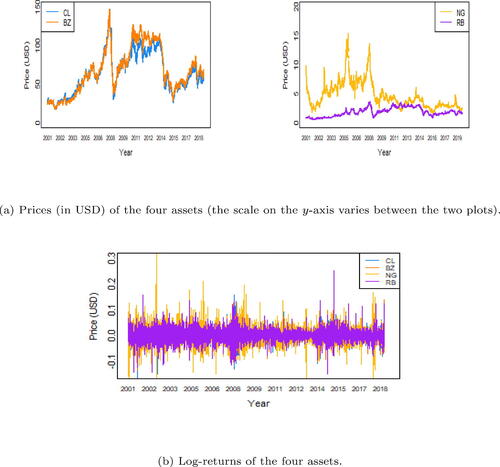
The 2008 global financial crisis has had strong effects on the global market, both short-term and long-term. In particular, it has affected commodity market prices (Chan et al., 2011). The crude oil market showed high volatility in the period after the financial crisis: while the crude oil prices constantly increased since the financialization of the commodity market in 2000, they fell from USD 133.88 in June 2008 to USD 39.09 in February 2009 (U.S. EIA, 2021), while natural gas fell from USD 12.69 to USD 4.52 in the same period (U.S. EIA, 2021). Figure 1(b) shows a strong fluctuation during 2008.

Fig. 1 Assets during the period of analysis.

Several studies have tried to investigate the effect of the global financial crisis on the oil market. Martina et al. (2011) used entropy to analyze oil market efficiency and suggested that extreme events should affect the market only short-term; Zhang et al. (2017) studied the correlation of crude oil and natural gas market volatility and identified a breakpoint in 2008 determing the change of volatility; Liu et al. (2020) showed that correlation between crude oil futures and sector ETFs increased since the 2008 financial crisis; Joo et al. (2020) examined the effect of the financial crisis on the oil market in terms of efficiency and long-term equilibrium. Often, studies focus on the immediate effect of the financial crisis, and not on the long-term changes in the oil market; moreover, even when focusing on long-term effects, as Joo et al. (2020), the interest is mainly on univariate time series.

This work aims at modeling the dependence structure among energy indices, including crude oil prices, crude oil derivatives, and natural gas. Immediately after the global financial crisis, the Organisation of the Petroleum Exporting Countries (OPEC) organized more frequent meetings, mostly aimed at reducing the oil production and this has been shown to negatively influence the oil market efficiency Jiang et al. (2014): the oil market needs time to react to new information. Since 2010, OPEC countries started to meet more regularly. We use the regularity of OPEC announcements as a variable (i) associated to the reduction of the volatility experienced after the financial crisis, and (ii) representing a factor that per se has an effect on the energy market.

We study the dependence structure of the energy asset prices depending on the regularity of OPEC announcements through copula models (Embrechts et al., 2001; Patton, 2012). There are several advantages in using copulas in this setting; first, the dependence structure can be flexibly described and does not have to be necessarily linear or symmetric, and it is possible to model the strenght of the dependnce among extreme values. Second, the marginal univariate time series can be modelled in a realistic way, by introducing ARCH effects, asymmetry and heavy tails, in case data show these characteristics, instead of using multivariate models with strong assumptions on both the univariate models and the multivariate dependence, which are often chosen for tractability. For both univariate models and copula models, we consider several choices and apply tools of model selection to identify the model which better represent the data. We show in this work that among the two considered time windows (when OPEC organized many extraordinary meetings and when OPEC organized more regular meetings) the tails of the univariate time series tended to become lighter, with extreme values less likely, and that the dependence among assets, measured as both monotonic dependence and tail dependence, decreased.

The remainder of the article is organized as follows. Section 2 introduces the background of energy prices analysis, Section 3 described the dataset used in this work, and the univariate and multivariate models that will be used to study the dependence structure among the assets; Section 4 discusses the results, and Section 5 concludes the article.

2 Background

OPEC is the largest and most prominent cartel in the world. It regularly hosts conferences among its thirteen members (Iran, Iraq, Kuwait, Saudi Arabia, Venezuela, Algeria, Angola, Congo, Equatorial Guinea, Gabon, Libya, Nigeria, and United Arab Emirates) to agree on oil production policies. Ordinary meetings of OPEC are held twice a year; however, extraordinary meetings can also been scheduled. The output of these meetings is usually an announcement, setting country-specific production quotas for its members (OPEC Secretariat, 2003). OPEC’s ability to influence the energy market has diminished over the years (Kaufmann et al., 2004); however, there is still evidence of a significant correlation between the oil prices and variables associated to OPEC (quotas, capacity utilization, excess of production quotas) (Fattouh, 2005; Guidi et al., 2006). In particular, there is evidence that OPEC announcements can have an impact on market volatility (Fattouh, 2005), for example, through the speculation about its decisions; nonetheless, the effect on energy prices time series is not fully understood yet.

The literature about the effect of OPEC announcements on crude oil markets or energy markets is still limited, and most of it focuses on univariate modelling. Draper (1984) studied the impact of scheduled and emergency OPEC announcements on different maturities separately, with some evidence of an effect of scheduled meetings but not of the unscheduled ones. Deaves and Krinsky (1992) classified the OPEC announcements into two groups (“good” and “bad”), depending on the effect on the returns of oil futures the day after the announcements and use models with ARCH effects to characterize the oil market, showing that “good” announcements have a positive effect on the market, while “bad” announcements have no significant effect. Wirl and Kujundzic (2004) used a more specific classifications of the announcements with a similar methology. Loutia et al. (2016) investigated the effect of OPEC production decisions, by classifying them into three categories (increase, cut, maintain), on both WTI and Brent crude oil prices by using separate EGARCH models. Guidi et al. (2006) analyzed the effect of OPEC production changes on stock returns in the United States and in the United Kingdom separately, and showed that reduction of the production seems to have a higher impact. Demirer and Kutan (2010) represents an attempt to analyze together spot and futures oil markets. All these works focus their interest on univariate time series; notably Klein (2018) studied the linear correlation between crude oil prices at different resolutions, showing that OPEC meetings have little impact on long-term price trends, but they can have an effect on the short-term trends for several days. In particular, negative trends tend to increase the volatility of crude oil prices, with respect to positive trends.

Our work is different from this literature because (i) we consider the regularity of OPEC announcements, (ii) we model the returns separately through GARCH models specific to each time series, and (iii) we combine the marginal models into a multivariate model through a copula function, in order to analyze the effect of the global finciancial crisis represented by the regularity of OPEC announcements on the dependence structure of energy-related returns.

Given the well-known limitations of linear correlation to describe dependence among financial returns (Embrechts et al., 2002), there is an extensive literature applying copulas to financial markets: see Patton (2006) and Ning (2010), among others, for analyses on the relationship between financial and exchange rate markets, and Reboredo (2011) for an application in the setting of crude oil prices. An important task when using copula models to study the dependence among asset prices is the choice of the particular copula function. In the early 2000’s, the Gaussian copula was a popular tool to model financial data in a flexible way, where individual time series of prices could follow several different marginal distributions. However, it is now recognized that Gaussian copulas, characterized by null tail dependence, can ignore the possibility of occurrence of extreme events (Malevergne and Sornette, 2003; MacKenzie and Spears, 2014). Alternative functions to the Gaussian copula are the Student-t copula, which is still an elliptical copula, or any copula function in the class of Archimedean copulas.

In the setting of energy market, Lu et al. (2014) used copulas with GARCH-type marginals to estimate the Value-at-Risk of crude oil prices and natural gas futures portfolios. Koirala et al. (2015) used copula models to measure the dependence between energy prices, including crude oil, gasoline and natural gas, and agricultural commodities, using a mixture of Clayton and Gumbel copulas to capture both lower and upper tail depdendence. Ji et al. (2018) studied the impact of uncertainties on energy prices through copula models, showing that there exists a negative dependence between energy returns and changes in the uncertainty. We are contributing to this literature by studying the effect of the regularity of OPEC announcements, as associated to the volatility induced by the global financial crisis, to study the changes in the dependence structure of energy prices, in terms of monotonic dependence, tail dependence, and distance from independence.

3 Methods and models

3.1 The data

We consider four assets to represent the energy market: daily prices of West Texas Intermediate (WTI, here indicated as CL) crude oil (originating from the Cushing Oil Field in Oklahoma) and Brent crude oil (originating from the Brent oilfields in the North Sea, here indicated as BZ), Reformulated Gasoline Blendstock for Oxygen Blending (RB), and natural gas (NG). OPEC produced oil is generally priced according to the Brent pricing benchmark, while North American produced oil typically uses the WTI pricing benchmark. RB is considered as a derivative of an OPEC controlled product. Finally, natural gas is considered as an energy asset which should not be influenced by OPEC.

The time series of BZ, CL, NG, and RB asset prices and the correponding log-returns are shown in Fig. 1(a) and 1(b). We used daily data available at the website https://www.backtestmarket.com. All assets’ dates are cross-matched to ensure the data series are synchronized with each other. Data refer to period from January 2001 through September 2019, with 4,608 data points. Table 1 provides descriptive statistics for the asset returns under analysis. The average log-returns are similar and the standard deviations are much larger than the corresponding means. Crude oil assets show a negative skewness, which can be interpreted as a tendency towards large decrease than large increase. Finally, the large values for the kurtosis statistics suggest distribution tails heavier than a normal distribution. Tables 2 and 3 show the sample Kendall’s τ and Spearman’s ρ for each pair of assets, which are measures of monotonic relationships among assets: as expected, the log-returns of the WTI and Brent are strongly correlated and RB is highly dependent on both WTI and Brent, being a derivative of crude oil. Finally NG seems to be only slightly correlated with the other assets.

Table 1 Descriptive statistics of the four asset returns.

Asset	Mean	SD	Max	Min	Skew.	Kurt.
BZ	2.068e-04	0.021	0.136	–0.134	–0.080	6.395
CL	1.668e-04	0.023	0.157	–0.165	–0.131	7.123
NG	–2.598e-04	0.033	0.324	–0.325	0.090	10.464
RB	1.596e-04	0.025	0.249	–0.150	0.116	8.404

Table 2 Sample Kendall’s τ for each pair of assets.

τ	BZ	CL	NG
CL	0.753	–	–
NG	0.164	0.161	–
RB	0.632	0.596	0.150

Table 3 Sample Spearman’s ρ for each pair of assets.

ρ	BZ	CL	NG
CL	0.902	–	–
NG	0.242	0.237	–
RB	0.811	0.777	0.221

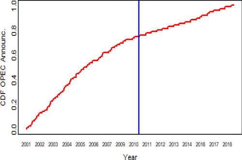
OPEC announcements for the same period are available at https://www.opec.org/opec_web/en/press_room/28.htm. We have decided to give equal weight to each release of new information on the movement of prices (decision of increase or decrease of OPEC’s production), in order to follow Jiang et al. (2014) and show that energy market needs time to process new information; therefore a dummy variable is introduced, which is equal to one when an announcement is made, independently from the type of decision made, and zero for no announcement. Figure 2 show the empirical cumulative distribution function for the binary time series: it can be noted that announcements occurred irregularly in the first period (Period 1), and regularly in the second one (Period 2); the blue line indicates the separation among the two periods. The changepoint has been inferred through a comparison in the means of the number of announcements per quarter: a t-test has been performed to compare the mean number of announcements in two consecutive quarters and the only significant difference correponded to the 37th quarters, which represents the first quarter of 2010. Therefore, we considered the changepoint in January 2010.

Fig. 2 Empirical CDF of the OPEC announcements with a change in the production.

3.2 Marginal models

It is well known that financial markets often exhibit time-varying volatility and this feature is well characterized by generalized autoregressive conditional heteroscedasticity (GARCH) models. Given a time series ${\left\{Y_t\right\}}_{t=0}^T$, its realization follows a GARCH(p, q) model if $$\begin{array}{c}{y}_t={\sigma }_t{\epsilon }_t\\ {\sigma }_t=\sqrt{{\alpha }_0+\sum _{i=1}^p{\alpha }_i{y}_{t-1}^2+\sum _{j=1}^q{\beta }_i{\sigma }_{t-j}^2},\end{array}$$where ${\epsilon }_t$ is a white noise, $p,q\ge 1$, and $\mathit{\alpha }=({\alpha }_1,\dots ,{\alpha }_p)$ and $\mathit{\beta }=({\beta }_1,\dots ,{\beta }_q)$ are parameters from an autoregressive (AR) and a moving average (MA) process, respectively; see Teräsvirta (2009) for a review.

There is evidence that crude oil price returns show heavy tails (Mohammadi and Su, 2010); therefore, we will consider a version of the GARCH(p, q) model with Student-t innovations, so that $y_t={\sigma }_t{\epsilon }_t$ where ${\epsilon }_t\sim t(\nu )$, that is, the error terms follows a t-distribution with ν degrees of freedom. It is possible to show that this model can be expressed via data augmentation (Geweke, 1993): $$\begin{array}{c}{y}_t={\epsilon }_t\sqrt{\frac{\nu -2}{\nu }{\omega }_t{\sigma }_t^2}\\ {\sigma }_t=\sqrt{{\alpha }_0+\sum _{i=1}^p{\alpha }_i{y}_{t-1}^2+\sum _{j=1}^q{\beta }_i{\sigma }_{t-j}^2}\\ {\epsilon }_t\sim \mathcal{N}(0,1)\\ {\omega }_t\sim IG\left(\frac{\nu }{2},\frac{\nu }{2}\right)\end{array}$$where IG(a, b) stands for the inverse gamma distribution with shape parameter a and scale parameter b.

Considering t-distributed innovations allows to fit leptokurtic data, since the kurtosis is associated with the number of degrees of freedom. However, the distribution still cannot deal with skewness, which may characterize financial data. Therefore, it is possible to consider ${\epsilon }_t$ from a skew-normal or a skew-t distribution (Salisu, 2016), by introducing a skewness parameter $\lambda >0$.

We will perform model selection to identify which GARCH model is the most suitable for each marginal distribution and to properly select the values of p and q. The main advantage to introduce a copula approach is that it allows to flexibly and realistically model each univariate time series separately and then model the dependence structure as a second step. In particular, GARCH models are known to suffer of the curse of dimensionality (Caporin and McAleer, 2014); however, we overcome this problem by modeling the time series relative to each asset separately and then relate them through a copula model.

There is evidence that misspecified marginal distributions can affect copula estimation, by increasing bias and mean-squared error (Azam, 2014; Fantazzini, 2009); however, this effect is particularly evident for small sample sizes, and it decreases as the length of the time series increases, as it is also empirically shown in Grazian and Liseo (2017). In order to check robustness with respect to the selected marginals, we will also implement copula estimation by using non parametric estimation of the marginals.

3.3 Copula models

Multivariate analysis can be affected by the assumptions implied in multivariate models. Multivariate distributions, such as the multivariate Gaussian distribution or the multivariate Student-t distribution, usually assume that all the marginal distributions have the same form; moreover, the dependence structure is often assumed to be linear, while in many settings there could be asymmetries, in particular in the tails of the multivariate distributions, or the relationship among processes can be more generally monotonic and not necessarily linear (Embrechts et al., 2002).

Copula models are representations of multivariate distribution which can take into account these generalizations. Given a random variable $\mathbf{Y}=(Y_1,\dots ,Y_d)$ with d-variate cumulative distribution function (CDF) F, Sklar’s theorem (Sklar, 1959) proves that there exists a d-variate function $C:{[0,1]}^d\stackrel{}{\to }[0,1]$ such that $$\mathbf{F}(y_1,\dots ,y_d;{\varphi }_1,\dots ,{\varphi }_d,\psi )=C(F_1(y_1;{\varphi }_1),\dots ,F_d(y_d;{\varphi }_d);\psi )$$where F_j is the marginal CDF of Y_j, indexed by marginal parameter ${\varphi }_j$ and ψ is the parameter characterizing the copula function. If F is continuous, it can be shown that this representation is also unique and, if F admits a density function f (1) $$\mathbf{f}(y_1,\dots ,y_d;{\varphi }_1,\dots ,{\varphi }_d,\psi )=c(F_1(y_1;{\varphi }_1),\dots ,F_d(y_d;{\varphi }_d);\psi )·f_1(y_1;{\varphi }_1)·\dots ·f_d(y_d;{\varphi }_d)$$(1) where c is the derivative of C; Eq. (1)(1) $$\mathbf{f}(y_1,\dots ,y_d;{\varphi }_1,\dots ,{\varphi }_d,\psi )=c(F_1(y_1;{\varphi }_1),\dots ,F_d(y_d;{\varphi }_d);\psi )·f_1(y_1;{\varphi }_1)·\dots ·f_d(y_d;{\varphi }_d)$$(1) shows that the copula function captures the full dependence structure of the multivariate joint distribution.

There are several copula functions available in the literature. Let define $u_j=F_j(y_j;{\varphi }_j)$ for $j=1,\dots ,d$. The Gaussian copula is defined as $$C_G(u_1,\dots ,u_d)=\mathbf{\Phi }({\Phi }^{-1}(u_1),\dots ,{\Phi }^{-1}(u_d);R)$$where $\mathbf{\Phi }$ is the CDF of a multivariate standard normal variable, ${\Phi }^{-1}$ is the inverse of a univariate standard normal CDF, and $\psi =R$ is a correlation matrix $R\in {[-1,1]}^{d\times d}$. The Gaussian copula has no tail dependence and it can be considered a generalization of the multivariate normal distribution, with marginal distribution that can be not-normal.

Similarly, the Student-t copula is defined as $$C_t(u_1,\dots ,u_d)=\mathbf{T}(T^{-1}(u_1;\nu ),\dots ,T^{-1}(u_d;\nu );\nu ,R)$$where T is a multivariate Student-t CDF, $T^{-1}$ is the inverse of a univariate Student-t CDF, and $\psi =(\nu ,R)$ where ν are the degrees of freedom and R is a correlation matrix, $R\in {[-1,1]}^{d\times d}$. Differently from the Gaussian copula, it allows symmetric non zero tail dependence (Schloegl and O’Kane, 2005). As for the marginal distributions, it is possible to extend the Student-t copula to allow for asymmetry, to obtain the skew-t copula: $$C_{\mathit{skewT}}(u_1,\dots ,u_d)=\mathit{skewT}(\mathit{skew}{T}^{-1}(u_1;{\delta }_1,\nu ),\dots ,\mathit{skew}{T}^{-1}(u_d;{\delta }_d,\nu );\nu ,R,\mathit{\delta }).$$ where $\psi =(\nu ,R,\mathit{\delta })$, ν being the number of degrees of freedom, R being a correlation matrix, and $\mathit{\delta }=({\delta }_1,\dots ,{\delta }_d)$ being a vector of skewness parameters. The multivariate skew-t distribution is defined as in Azzalini and Capitanio (2003).

Copula functions showing asymmetric tail dependence are the Clayton and the Gumbel copulas. The Clayton copula is defined as $$C(u_1,\dots ,u_d)={\left[\sum _{j=1}^d{u}_j^{-\theta }-d+1\right]}^{-\frac{1}{\theta }}$$where $\psi =\theta$ with $\theta \in [-1,\infty )\setminus \left\{0\right\}$; the Clayton copula shows positive dependence in the lower tail and no dependence in the upper tail. On the contrary, the Gumbel copula is defined as $$C(u_1,\dots ,u_d)=\hspace{0.17em}\exp \hspace{0.17em}\left[-{\left(\sum _{j=1}^d{(-\hspace{0.17em}\log \hspace{0.17em}{u}_j)}^{\theta }\right)}^{\frac{1}{\theta }}\right],$$ with $\psi =\theta$ and $\theta \in [1,\infty )$; the Gumbel copula shows positive dependence in the upper tail and no dependence in the lower tail. Another example of Archimedean copula showing no tail dependence is the Frank copula, defined as $$C(u_1,\dots ,u_d)=\frac{1}{\theta }\log \hspace{0.17em}\left[1+\frac{\prod _{j=1}^d\hspace{0.17em}\exp \hspace{0.17em}(-\theta u_j)-1}{{[\exp \hspace{0.17em}(-\theta )-1]}^{d-1}}\right]$$ with $\psi =\theta$ and $\theta \in \mathbb{R}\setminus \left\{0\right\}$.

Copula models can be made more complex, by introducing dependence on a covariate (Patton, 2006). The most important extension is considering time-varying copula parameters, that is, the copula parameters is allowed to vary with time according to some model (Aielli, 2013; De Lira Salvatierra and Patton, 2015).

In many settings, some functionals of the dependence are of interest. In the following, we introduce bivariate functionals; extensions to the multivariate settings exist, however they may not be uniquely defined. The Spearman’s ρ between two variables Y₁ and Y₂ is the correlation coefficient among the transformed variables $U=F_1(y_1)$ and $V=F_2(y_2)$, assessing the relationship among the two variables as a monotonic function; it has a copula definition $${\rho }_S=12{\int }_0^1{\int }_0^{1}C(u,v)\mathit{dudv}-3.$$

Similarly, the Kendall’s τ is another measure of rank correlation defined as $$\tau =4{\int }_0^1{\int }_0^{1}C(u,v)dC(u,v)-1.$$

Both the Spearman’s ρ and the Kendall’s τ are invaritant under monotone transformations and they range in $[-1,1]$, where the sign of the index indicates the direction of the association between variables.

The Spearman’s ρ and the Kendall’s τ are equal to zero if the variables are independent, however the fact that $\rho =\tau =0$ does not imply that the variables are independent. Moreover, these indices may be equal for different families of copula models: for example, the Kendall’s τ are equal for all elliptical families (Fang et al., 2002) and the Spearman’s ρ is the same for the Student-t and the Gaussian copula.

On the other hand, the mutual information measures the divergence between the joint distribution represented by a copula and the model of independence, represented by the product of the marginals and can assume different values for different families of copulas, depending on the strength of the dependence (Ebrahim et al., 2014). The mutual information Granger and Lin (1994) for continuous random variables is defined in terms of the Kullback-Leibler divergence or the Shannon entropy $H(·)$ $$\begin{array}{c}I(Y_1,Y_2)=\int \int f(y_1,y_2)\hspace{0.17em}\log \hspace{0.17em}\left(\frac{f(y_1,y_2)}{f_1(y_1)·f_2(y_2)}\right)d{y}_{1}d{y}_2\\ =H(Y_1)+H(Y_2)-H(Y_1,Y_2).\end{array}$$

The mutual information has also a copula representation, which makes use of the simplification for which $H(U_i)=0$ $$\begin{array}{c}I(U_1,U_2)={\int }_{[0,1]}{\int }_{[0,1]}c(u_1,u_2)\hspace{0.17em}\log \hspace{0.17em}c(u_1,u_2)d{u}_{1}d{u}_2\\ =-H(U_1,U_2)=I(C),\end{array}$$where I(C) is called the information function of the copula (Ebrahim et al., 2014). Given the definition of mutual information in terms of Shannon entropy, it is possible to use entropy expressions for multivariate distributions to easily obtain expression for the mutual information; see, for example, Nadarajah and Zografos (2005) and Darbellay and Vajda (2000).

The mutual information index for absolutely continuous distributions is (2) $${\delta }^2(C)=1-e^{-2I(Y_1,Y_2)}.$$(2)

The mutual information index ranges in $[0,1]$. Alternatively, the normalized version of the Bhattacharya-Matusita-Hellinger measure of dependence is defined as $$S_{\rho }=\frac{1}{2}{\int }_{\mathcal{Y}}{\int }_{\mathcal{Y}}{\left(c^{1/2}(F_1(y_1),F_2(y_2))-{(f_1(y_1)·f_2(y_2))}^{1/2}\right)}^{2}d{y}_{1}d{y}_2$$where c is the joint copula density and f_j is the marginal density of the j-th variable, j = 1, 2. The index $S_{\rho }$ is equal to zero if and only if $C=F_1·F_2$. Granger et al. (2004) show that $S_{\rho }$ has also a copula representation as $$S_{\rho }={\int }_{[0,1]}{\int }_{[0,1]}[1-c^{1/2}(u_1,u_2)]d{u}_{1}d{v}_2.$$

The Bhattacharya-Matusita-Hellinger measure of dependence is a non parametric measure of dependence which is robust to non linearity of the observations, and measures the departure from independence. Geenens and Lafaye de Micheaux (2022) defined a Hellinger correlation coefficient as (3) $${\mathcal{H}}^2=1-{\int }_{[0,1]}{\int }_{[0,1]}\sqrt{c(u_1,u_2)}d{u}_{1}d{u}_2$$(3) and found an L₂-consistent estimator, which will be used in this work.

Finally, it is important to test if random vectors can be assumed mutually independent, in order to characterize the dependence structure as a multivariate distribution or, more easily, as a combination of bivariate distributions. Bakirov et al. (2006) proposed a distance correlation based on functionals of the characteristic functions, which can deal with variables of different nature. We will use it to test mutual indpependence of random vectors. Consider Y₁ as a random vector in ${\mathbb{R}}^{d_1}$ and Y₂ a random vector in ${\mathbb{R}}^{d_2}$, where d₁ and d₂ are positive integers. Define the characteristic functions of Y₁ and Y₂ as $g_{Y_1}$ and $g_{Y_2}$, respectively, and the joint characteristic function as $g_{Y_1,Y_2}$. The measure $$\begin{array}{c}{\mathcal{V}}^2(Y_1,Y_2;w)=\parallel g_{Y_1,Y_2}-g_{Y_1}·g_{Y_2}{\parallel }_w^2\\ ={\int }_{{\mathbb{R}}^{d_1+d_2}}|g_{Y_1,Y_2}(y_1,y_2)-g_{Y_1}(y_1)g_{Y_2}(y_2){|}^{2}w(y_1,y_2)d{y}_{1}d{y}_2\end{array}$$between the joint characteristic function and the product of the marginal characteristic functions (where $\parallel ·\parallel$ indicates the norm and w is a weight function) can be used to test the hypothesis of independence $$\begin{array}{c}{H}_0:g_{Y_1,Y_2}=g_{Y_1}·g_{Y_2}\\ H_1:g_{Y_1,Y_2}\ne g_{Y_1}·g_{Y_2}.\end{array}$$

The measure ${\mathcal{V}}^2$ has the property to be zero if and only if Y₁ and Y₂ are independent. Székely et al. (2007) studied the theoretical properties of this test statistic, in particular consistency.

Finally, some studies show that, in particular in presence of volatile markets, tail dependence is useful to study the behavior of extremes in finance (Ane and Kharoubi, 2003). Differently from rank correlations, tail dependence indices describe the concordance in the tails of the bivariate distribution, that is, the dependence of crude oil markets to move together up or down: (5) $${\lambda }_U=\underset{v\to 1^{-}}{\lim }\mathrm{Pr}(F_1(y_1)>v|F_2(y_2)>v)=\underset{v\to 1^{-}}{\lim }\frac{1-2v+C(v,v)}{1-v}$$(5) (6) $${\lambda }_L=\underset{v\to 0^{+}}{\lim }\mathrm{Pr}(F_1(y_1)\le v|F_2(y_2)\le v)=\underset{v\to 0^{+}}{\lim }\frac{C(v,v)}{u}$$(6) provided that the limits exist. Equation (5)(5) $${\lambda }_U=\underset{v\to 1^{-}}{\lim }\mathrm{Pr}(F_1(y_1)>v|F_2(y_2)>v)=\underset{v\to 1^{-}}{\lim }\frac{1-2v+C(v,v)}{1-v}$$(5) represents the upper tail dependence index, while Eq. (6)(6) $${\lambda }_L=\underset{v\to 0^{+}}{\lim }\mathrm{Pr}(F_1(y_1)\le v|F_2(y_2)\le v)=\underset{v\to 0^{+}}{\lim }\frac{C(v,v)}{u}$$(6) represents the lower tail dependence index.

3.4 Methods for inference and testing

Inferential approaches to parameter estimation for copula models often rely on a two-step procedure (Patton, 2004; Cherubini et al., 2004; Kim et al., 2007; Nikoloulopoulos et al., 2008): first parameters of the univariate marginals are estimated from separate univariate likelihoods and then the parameter of the copula model is estimating by pluggin-in the estimates obtained from the first step into the multivariate likelihood. Such approach allows for asymptotic normality and consistency (Francq and Zakoian, 2004). Joe (2005) studied the efficiency of the two-step procedure, showing good efficiency except for the cases of extreme dependence, which does not seem to be the case of the application under analysis, see Section 4. More specifically, under regularity conditions, the relative efficiency of the two-step estimator with respect to the full likelihood estimator tends to one in case of independence of the marginals, and reaches its minimum in case of perfect dependence.

The two-step procedure presents the flexibility to choose the model that best fit each time series. For a time series of length T, with observed random vectors ${\mathbf{y}}_1,\dots ,{\mathbf{y}}_d$, there are d log-likelihood functions for the univariatiate marginals: $${\mathcal{l}}_j({\varphi }_j)=\sum _{t=1}^T\hspace{0.17em}\log \hspace{0.17em}{f}_j(y_{j,t};{\varphi }_j)\mathrm{\hspace{1em}}\mathrm{\hspace{1em}}j=1,\dots ,d$$and the log-likelihood for the joint distribution is: $$\begin{array}{c}\mathcal{l}({\varphi }_1,\dots ,{\varphi }_d,\psi ;{\mathbf{y}}_1,\dots ,{\mathbf{y}}_d)=\sum _{t=1}^T[\log \hspace{0.17em}{f}_1(y_{1,t};{\varphi }_1)+\dots +\hspace{0.17em}\log \hspace{0.17em}{f}_d(y_{d,t};{\varphi }_d)\\ \mathrm{\hspace{1em}}\mathrm{\hspace{1em}}+\hspace{0.17em}\log \hspace{0.17em}c(u_{1,t},\dots ,u_{d,t};\psi )]\end{array}$$ where ${\varphi }_j$ represents the vector of parameters of the marginal distributions for $j=\{1,\dots ,d\}$ and ψ represents the vector of parameter of the copula function; $u_{j,t}=F_j(y_{j,t};{\varphi }_j)$ are the pseudo-observations. Performing a fully maximum-likelihood approach requires an increasing level of computational difficulty as the dimension increases, therefore the two-stage procedure can be implemented. The two-stage procedure is performed by first estimating the parameters of the marginal distributions to obtain estimates $({\widehat{\varphi }}_1,\dots ,{\widehat{\varphi }}_d)$ and, therefore, ${\widehat{f}}_j(y_{j,t};{\widehat{\varphi }}_j)$; then define ${\widehat{u}}_{j,t}={\widehat{F}}_j(y_{j,t};{\widehat{\varphi }}_j)$ and estimate: $$\widehat{\psi }=\arg \underset{\psi \in \Psi }{\max }\sum _{t=1}^T\hspace{0.17em}\log \hspace{0.17em}c\left({\widehat{u}}_{1,t},\dots ,{\widehat{u}}_{d,t};\psi \right).$$

Under regularity conditions, $({\widehat{\varphi }}_1,\dots ,{\widehat{\varphi }}_d,\widehat{\psi })$ is the solution of $$\left(\frac{\partial {\mathcal{l}}_1}{\partial {\varphi }_1^T},\dots ,\frac{\partial {\mathcal{l}}_d}{\partial {\varphi }_d^T},\frac{\partial \mathcal{l}}{\partial {\psi }^T}\right)={\mathbf{0}}^T$$which is, in general, different from the maximum likelihood estimators given by the solutions to $$\left(\frac{\partial \mathcal{l}}{\partial {\varphi }_1^T},\dots ,\frac{\partial \mathcal{l}}{\partial {\varphi }_d^T},\frac{\partial \mathcal{l}}{\partial {\psi }^T}\right)={\mathbf{0}}^T.$$

Selecting the correct model under the marginals may not be an easy task. In order to reduce the impact of model assumptions, several models can be compared for both the marginal distributions and the joint distribution, and model selection measures used to select the best model; for example, BIC (Bayesian information criterion) is often applied in this setting. However, selection criteria may disagree and sometimes there is not enough information to select a model with a reasonable degree of confidence. Fantazzini (2009) studied the effect of misspecification of the marginals on the copula estimation: in particular, Fantazzini (2009) found via simulation that, when observations are characterized by skewness and symmetric marginals are assumed together with a Gaussian copula, correlations are negatively biased; the bias seems to increase when the true copula is a Student-t copula and marginals do not properly account for skewness. Moreover, bias is still evident when the true copula generating the data is not elliptical and marginals do not account for skewness, although the sign of the bias may differ.

Genest et al. (1995) proposed a semiparametric approach, where non parametric estimates are obtained for the marginal distributions, while a parametric model is assumed for the copula. Then the copula parameter ψ is estimated as that value $\widehat{\psi }$ that maximizes the pseudo log-likelihood $$\mathcal{l}(\psi ;{\mathbf{y}}_1,\dots ,{\mathbf{y}}_d)=\sum _{t=1}^T\hspace{0.17em}\log \hspace{0.17em}\left[c\left({\widehat{F}}_{1n}(y_{1,t}),\dots ,{\widehat{F}}_{dn}(y_{d,t})\right)\right]$$where ${\widehat{F}}_{jn}(y_{j,t})=\frac{1}{T+1}{\sum }_{t=1}^T\mathbb{I}[Y_{j,t}<y_{j,t}]$ is the marginal empirical CDF of the j-th variable. The denominator is taken to be equal to $(T+1)$ so that difficulties arising when the estimates are close to one are avoided. The semiparametric approach can be more flexible because it does not need to choose the marginal parametric families and is more robust to model misspecification. The semiparametric estimator of the copula parameter is not as efficient as the maximum likelihood estimator (Genest et al., 1995); however, Genest and Werker (2002) studied the conditions for which it is asymptotically efficient. Kim et al. (2007) showed through simulations that, when marginals are misspecified, the mean squared error obtained by applying the two-step parametric procedures (and also the fully maximum likelihood approach) can be large, with respect to the semiparametric procedure, which is not computationally more expensive.

In this work, we compare the results obtained by using either a fully parametric and a semiparametric approach.

4 Results

4.1 Marginal models

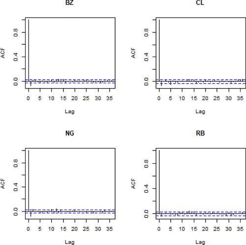
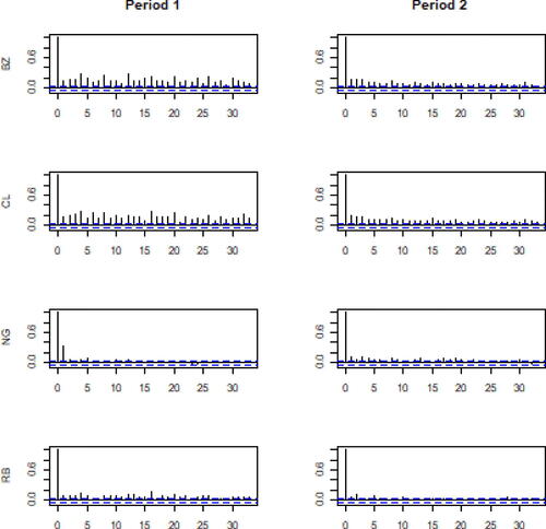
First, log-returns for all time series have been tested for heteroscedasticity by using the Engle’s ARCH test (Engle, 1982); the test rejects the null hypothesis of no heteroscedasticity at lag m for a significance level of 0.05. Similarly, we have applied the Ljung-Box Q-test (Ljung and Box, 1978) for testing for autocorrelation and the null hypothesis of no autocorrelation at lag m is rejected at a significance level of 0.05. Both tests have been applied for every lag $m\in \{1,2,\dots ,200\}$; the Engle’s ARCH test confirms persistence of heteroskedasticity for every time series at large lag (p-value of order ${10}^{-16}$); on the other hand, the Ljung-Box test for the hypothesis of independence in each times series shows no autocorrelation after lag m = 1 for BZ (p-value of order ${10}^{-6}$), CL (p-value of order ${10}^{-5}$), NG (p-value of order ${10}^{-8}$), and after lag m = 13 for RB (p-value of order ${10}^{-6}$). Figure 3 shows the autocorrelation plots for each series, suggesting that autocorrelation is not significantly different from zero after lag m = 1; moreover, for RB autocorrelation, even if tested present, seems to be low.

Fig. 3 Autocorrelation plots for the four log-returns time series.

Figures 4 and 5 show the autocorrelation plots of the absolute value and the squared value of the time series of the four log-returns in the two time windows to investigate the persistence of volatility: they both agree that autocorrelation seems to remain at large lag, in particular for BZ and CL.

Fig. 4 Autocorrelation plots for the absolute value of the four time series.

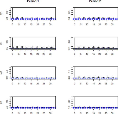
Fig. 5 Autocorrelation plots for the square value of the four time series.

In order to test for heavy tails, the Hill’s estimator has been computed for each time series: $$\widehat{\alpha }={\left[\frac{1}{k}\sum _{i=1}^{k-1}\hspace{0.17em}\log \hspace{0.17em}(y_{T-i}-\hspace{0.17em}\log \hspace{0.17em}(y_{T-k}))\right]}^{-1}$$where k is the number of upper-order statistics used in the estimation. 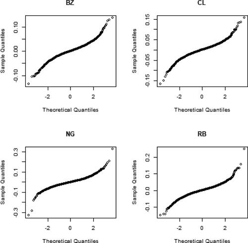Figure 6 shows the obtained plots for values of $k\in \{1,\dots ,1000\}$, showing that the estimates of the Hill’s index are always larger than zero, for all the considered values of k. Moreover, Fig. 7 shows the qq-plots for each time series, from which it is evident that the tails of each time series do not allow for a Gaussian assumption.

Fig. 6 Plots of the Hill’s estimators computed for different values of the upper-order statistics k.

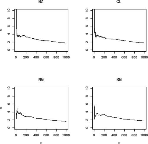
Fig. 7 Qq-plots of the four time series.

We have fitted GARCH(p, q) models with Gaussian and Student-t innovation, and allowing or not for skewness, with parameters p and q ranging from 0 to 10. The best model for each time series has been selected via Bayesian information criterion (BIC) for all models, see Table 4; for reasons of space, only values of $p\in \{1,2\}$ and $q\in \{0,1,2\}$ are shown, since the values of BIC for all the other models where larger. In all cases, models with p = 1 and q = 1 and Student-t innovations are preferred, which means that extreme returns are more likely than in the Gaussian case. Moreover, the time series of BZ and CL in the second time window and of NG in both time windows seem to show asymmetry, with a preference for skew-t models. It is also possible to see from Table 4 that the BIC values are similar for all models, which means that data are not strongly supporting the selected models against the others. For this reason, in Section 4.2 a comparison between parametrically estimated marginal and non parametrically estimated marginals and their effect on the estimation of the copula parameters and the dependence measures is provided.

Table 4 BIC values for combinations of p and q in GARCH models of log-returns for Gaussian, skew-normal, Student-t, and skew-t innovations.

	Period 1	q $=0$	q $=1$	q $=2$	Period 2	q $=0$	q $=1$	q $=2$
BZ							Gaussian
	p $=1$	–4.713	–4.844	–4.841	p $=1$	–5.093	–5.252	–5.248
	p $=2$	–4.744	–4.840	–4.837	p $=2$	–5.126	–5.248	–5.245
							skew-Gaussian
	p $=1$	–4.711	–4.842	–4.839	p $=1$	–5.091	–5.257	–5.254
	p $=2$	–4.742	–4.838	–4.835	p $=2$	–5.124	–5.253	–5.250
							Student-t
	p $=1$	–4.774	–4.852	–4.848	p $=1$	–5.229	–5.329	–5.327
	p $=2$	–4.784	–4.848	–4.845	p $=2$	–5.250	–5.326	–5.323
							skew-t
	p $=1$	–4.771	–4.849	–4.845	p $=1$	–5.228	–5.330	–5.327
	p $=2$	–4.781	–4.845	–4.842	p $=2$	–5.249	–5.327	–5.324
CL							Gaussian
	p $=1$	–4.547	–4.692	–4.691	p $=1$	–4.947	–5.094	–5.090
	p $=2$	–4.585	–4.689	–4.687	p $=2$	–4.992	–5.090	–5.088
							skew-Gaussian
	p $=1$	–4.546	–4.693	–4.691	p $=1$	–4.946	–5.102	–5.099
	p $=2$	–4.587	–4.690	–4.688	p $=2$	–4.992	–5.099	–5.096
							Student-t
	p $=1$	–4.624	–4.712	–4.708	p $=1$	–5.044	–5.149	–5.145
	p $=2$	–4.636	–4.709	–4.706	p $=2$	–5.070	–5.145	–5.143
							skew-t
	p $=1$	–4.621	–4.709	–4.706	p $=1$	–5.047	–5.155	–5.151
	p $=2$	–4.633	–4.707	–4.703	p $=2$	–5.073	–5.151	–5.148
NG							Gaussian
	p $=1$	–3.738	–3.806	–3.804	p $=1$	–4.370	–4.509	–4.506
	p $=2$	–3.747	–3.803	–3.800	p $=2$	–4.377	–4.508	–4.505
							skew-Gaussian
	p $=1$	–3.744	–3.813	–3.810	p $=1$	–4.367	–4.507	–4.503
	p $=2$	–3.754	–3.810	–4.808	p $=2$	–4.375	–4.506	–4.502
							Student-t
	p $=1$	–3.824	–3.872	–3.869	p $=1$	–4.461	–4.529	–4.526
	p $=2$	–3.833	–3.871	–3.868	p $=2$	–4.473	–4.531	–4.528
							skew-t
	p $=1$	–3.822	–3.873	–3.870	p $=1$	–4.458	–4.530	–4.522
	p $=2$	–3.832	–3.872	–3.868	p $=2$	–4.470	–4.526	–4.525
RB							Gaussian
	p $=1$	–4.289	–4.348	–4.345	p $=1$	–4.911	–5.006	–5.002
	p $=2$	–4.295	–4.345	–4.342	p $=2$	–4.942	–5.003	–5.006
							skew-Gaussian
	p $=1$	–4.290	–4.347	–4.344	p $=1$	–4.908	–5.003	–4.999
	p $=2$	–4.295	–4.344	–4.340	p $=2$	–4.938	–5.000	–5.003
							Student-t
	p $=1$	–4.347	–4.386	–4.383	p $=1$	–5.067	–5.115	–5.112
	p $=2$	–4.350	–4.383	–4.379	p $=2$	–5.074	–5.112	–5.108
							skew-t
	p $=1$	–4.346	–4.385	–4.381	p $=1$	–5.067	–5.114	–5.111
	p $=2$	–4.350	–4.382	–4.378	p $=2$	–5.072	–5.111	–5.107

The selected model (the model with the lowest BIC) is given in bold. Models with p > 2 and q > 2 are not provided because they are associated with larger BIC values.

Table 5 shows the maximum likelihood estimates of the parameters of marginal models selected as in Table 4, in the period before and after the change in the regularity of the OPEC announcements. The possibility to separately model the marginal distributions, which is an essential part of the copula approach, allows to use the models that show the better fit to the marginal data: for example, it is possible to use models with asymmetry for BZ and CL in Period 2 and NG in both Periods, and models without asymmetry for the other time series. Moreover, it is possible to model the log-returns with flexible models, as the GARCH-skew-t model, without incurring in the curse of dimensionality previously described, since we only model the one-dimensional distributions.

Table 5 Parameter maximum likelihood estimates for the models selected as optimal models with BIC as in Table 4 (standard errors in brackets).

BZ	Period 1	Period 2	CL	Period 1	Period 2
α 0	7.908e-06	2.011e-06	α0	8.529e-06	2.614e-06
	(2.937e-06)	(3.114e-04)		(2.911e-06)	(1.163e-06)
α1	0.049	0.061	α1	0.047	0.060
	(0.010)	(0.012)		(0.009)	(0.010)
β1	0.935	0.937	β1	0.938	0.937
	(0.013)	(0.011)		(0.001)	(0.010)
ν	10.000	5.427	ν	10.000	6.520
	(1.590)	(0.599)		(1.599)	(0.925)
λ	–	0.921	λ	–	0.874
	–	(0.026)		–	(0.025)
NG	Period 1	Period 2	RB	Period 1	Period 2
α0	3.451e-05	1.685e-05	α0	1.111e-05	2.461e-06
	(1.034e-05)	(4.633e-06)		(4.835e-06)	(1.199e-06)
α1	0.071	0.076	α1	0.033	0.027
	(0.012)	(0.011)		(0.008)	(0.007)
β1	0.906	0.901	β1	0.953	0.968
	(0.014)	(0.013)		(0.012)	(0.009)
ν	6.074	9.472	ν	7.242	4.841
	(0.740)	(1.647)		(1.015)	0.459
λ	1.095	1.024	λ	–	–
	(0.032)	(0.003)		–	–

α₀ is the location of the volatility model, α₁ and β₁ are the coefficient of the AR part and the MA part respectively, ν is the number of degrees of freedom for Student-t innovations, and λ is the parameter of asymmetry for skewed innovations.

The comparison among periods shows that there are slight differences among the parameters of each univariate distribution; the parameters which shows the largest change in the estimation is the number of degrees of freedom ν. It is interesting to notice that the number of degrees of freedom for BZ, CL and RB is decreasing between the two time windows, while it is increasing for NG. The number of degrees of freedom in a Student-t or skew-t distribution is associated with the kurtosis of the distribution: lower values of ν are associated with leptokurtic distributions (heavy tails) and larger values of ν are associated with vanishing kurtosis. The results show that heavier tails are more suitable for model crude oil prices in the second time window, while NG shows lighter tails. With a copula approach, it is possible to separately estimate the degrees of freedom of each time series and it is then possible to flexibly model the tails of each univariate distribution.

4.2 Copula model

We now analyze the change in the dependence structure among the four assets considered in this work before and after the change in the regularity of the OPEC announcements. First, we investigate the structure of mutual independence of the four assets with the test proposed by Bakirov et al. (2006) and Székely et al. (2007) and defined in Eq. (4). The test statistic ${\mathcal{V}}^2$ is 0.501 when testing the independence between the bivariate distribution of BZ and CL and the bivariate distribution of NG and RB (p-value: 0.001), 0.523 for BZ-NG versus CL-RB (p-value: 0.001), and 0.530 for CL-NG versus BZ-RB (p-value: 0.001), suggesting that also the bivariate distributions are dependent. Similarly, the test statistic is 0.524 (p-value: 0.001) for the trivariate distribution of (BZ,CL,NG) against the univariate distribution of RB, 0.577 (p-value: 0.001) for (CL,NG,RB) against BZ, 0.092 (p-value: 0.001) for (BZ,CL,RB) against NG, and 0.572 (p-value: 0.001) for (BZ,NG,RB) against CL, again suggesting dependence among the trivariate distributions and the univariate distributions.

We have fit six different copula models (Gaussian, Student-t, skew-t, Clayton, Frank, and Gumbel copula). Table 6 shows the BIC values for the considered copula function for the four-dimensional distribution of the four log-returns time series, obtained with non parametric estimation of the marginal distributions. In both periods, the selected copula models is a t-copula and the estimates for the correlation matrix R is available in Table 7: it is possible to notice a reduction of the correlation between Period 1 and Period 2, in particular for those pairs of assets involving NG (for which the correlation is already low in Period 1). The number of degrees of freedom passes from 5.427 estimated in Period 1, to 5.139 estimated in Period 2.

Table 6 BIC values for several copula functions for the four-dimensional distribution of the four assets.

Period 1	BIC	Period 2	BIC
Gaussian	–3800.966	Gaussian	–2611.677
t	–4571.084	t	–7391.888
skew-t	–2918.942	skew-t	–4345.774
Clayton	–3132.900	Clayton	–2469.057
Frank	–3450.927	Frank	–2306.257
Gumbel	–3439.927	Gumbel	–2209.688

The bold values are relative to the smallest value of BIC.

Table 7 Values of the R correlation matrix of the t copula selected in Table 6.

				Period 1					Period 2
	BZ	CL	NG	RB		BZ	CL	NG	RB
BZ	1.000	0.945	0.313	0.806	BZ	1.000	0.922	0.121	0.871
CL		1.000	0.312	0.808	CL		1.000	0.125	0.811
NG			1.000	0.290	NG			1.000	0.110
RB				1.000	RB				1.000

In this work, the interest is focused on functionals of bivariate dependence. Extensions to multivariate cases exist but they may not be unique; this reflects the fact that various dependence structures can exist in the multivariate setting: consider, for example, mutual independence between all variables, independence between two subsets of variables, pariwise independence, conditional independence, etc. Therefore, functionals of dependence can be defined with respect to the multivariate copula, in relation to the independence copula, or as weighted averages of pairwise functionals; see, for example, Schmid and Schmidt (2007). Alternatively, it is possible to use the mutual information among all variables, which involves expressions for the entropy, as described in Section 3.3. Given the additional challenges in exploring the structure of multivariate dependence, we focus on the pairwise functionals in this work, and leave other multivariate aspects for further research.

We fit the same six copula models for each pair of assets, such that $${\widehat{\psi }}_{jk}=\arg \underset{{\psi }_{jk}\in \Psi }{\max }\sum _{t=1}^T\hspace{0.17em}\log \hspace{0.17em}c\left({\widehat{u}}_{j,t},{\widehat{u}}_{k,t};{\psi }_{jk}\right).$$for $j,k=\{BZ,CL,RB,NG\}$ and where ${\widehat{u}}_{j,t}$ are the pseudo-observations obtained either by plugging it the parameter estimates of the marginal models or as empirical CDF estimates; the parameter ψ varies according to the specific copula model: for the Gaussian copula, $\psi =\rho$, where ρ is the correlation parameter between the two assets; for the Student-t copula, $\psi =(\rho ,\nu )$, where ρ is the correlation coefficient between the two assets and ν is the number of degrees of freedom; for the skew-t copula, $\psi =(\rho ,\delta ,\nu )$ where ρ is the correlation parameter between the two assets, ν is the number of degrees of freedom, and δ is the skewness parameter; for the Clayton, Gumbel, and Frank copulas $\psi =\theta$ where θ is the parameter for each of the Archimedean copulas.

For each copula, we have computed the BIC to select the best model (Tables 8 and 9). We implemented also dynamic-copula models, where the parameters of the copula are allowed to vary over time, using the Dynamic Copula Toolbox 3.0(Vogiatzoglou, 2021). In every case, the non dynamic version was preferred according to the BIC; therefore, we have omitted those results. Table 8 shows the BIC values when marginals are non parametrically estimated, while Table 9 shows the BIC values for copula models when marginals are parametrically estimated: it is possible to see that the same model is selected in all cases, which means that, in this particular example, the parametric estimation of the marginals seems to be robust to the selection of the copula model.

Table 8 BIC competing copula models with non parametric estimation of the marginals.

	Gaussian	Student-t	Skew-t	Clayton	Frank	Gumbel
						Period 1
BZ–CL	–4117.66	–5190.26	–2794.03	–3894.68	–4354.94	–4593.52
BZ-NG	–310.65	–321.23	–189.90	–120.56	–300.48	–298.49
BZ-RB	–2429.25	–2619.31	–1110.50	–1990.35	–2286.32	–2427.56
CL-NG	–290.38	–302.15	–188.33	–167.23	–287.10	–269.34
CL-RB	–2364.18	–2652.75	–1559.21	–1976.45	–2316.80	–2434.86
NG-RB	–264.13	–278.10	–207.81	–51.67	–246.97	–243.21
						Period 2
BZ-CL	–4031.15	–4391.16	–2454.40	–3712.93	–3755.15	–4037.03
BZ-NG	–25.59	–27.75	–10.60	–41.40	–19.87	–15.94
BZ-RB	–2796.11	–3097.66	–1738.28	–2475.06	–2833.84	–2826.30
CL-NG	–25.26	–31.88	–10.96	–50.26	–20.15	–13.33
CL-RB	–2118.41	–2284.69	–945.29	–1873.64	–2039.89	–2077.77
NG-RB	–20.55	–25.47	–8.91	–31.56	–13.07	–17.61

Table 9 BIC competing copula models with parametric estimation of the marginals, with the best model chosen as in Table 8.

	Gaussian	Student-t	Skew-t	Clayton	Frank	Gumbel
						Period 1
BZ-CL	–4417.92	–5561.25	–5558.12	–4261.75	–4897.02	–4922.33
BZ-NG	–293.28	–300.42	–294.58	–199.84	–294.88	–282.30
BZ-RB	–2642.27	–2841.43	–2835.09	–2180.52	–2668.69	–2606.24
CL-NG	–268.89	–278.71	–271.11	–196.40	–273.92	–251.74
CL-RB	–2551.66	–2872.38	–2865.59	–2171.51	–2668.63	–2610.65
NG-RB	–251.17	–258.80	–251.12	–191.64	–248.26	–229.97
						Period 2
BZ-CL	–3606.11	–3923.62	–2924.94	–3283.16	–3241.28	–3599.84
BZ-NG	–24.10	–21.01	–26.27	–41.90	–18.43	–8.18
BZ-RB	–2471.42	–2779.69	–2774.71	–2193.09	–2391.46	–2522.41
CL-NG	–27.11	–27.50	–40.62	–54.05	–22.18	–7.52
CL-RB	–1841.31	–1996.09	–1994.79	–1628.17	–1690.92	–1801.72
NG-RB	–18.17	–13.61	–13.31	–29.26	–11.46	–7.71

The Student-t copula is chosen as the best model for most of the pairs of assets in Period 1. In the second period, the Student-t is the best model for asset pairs not involving NG, and the Clayton copula is the best for asset pairs involving NG. The latter model suggests that in the second period, pair of assets involving NG show no upper tail dependence. However, these are cases where the dependence is quite weak, in general.

Table 10 shows the point estimates and the relative standard errors of the model selected as optimal by BIC for each pair of assets. Gaussian, Gumbel, Frank, and skew copulas are not shown in Table 10 because they were never selected. Table 10 provides estimates obtained with non parametric estimation of the marginals; results obtained with parametric estimation of the marginals were very similar and, for this reason, omitted.

Table 10 Parameters estimates for the copula models chosen according to Table 9 and Table 8, and corresponding standard errors (in italic).

			Period 1			Period 2
	Student-t		Clayton	Student-t		Clayton
	ρ	ν	θ	ρ	ν	θ
BZ-CL	0.947	1.976	–	0.918	2.393	–
	(0.017)	(3.003)		(0.004)	(0.241)
BZ-NG	0.327	13.515	–	–	–	0.202
	(0.017)	(3.546)				(0.032)
BZ-RB	0.839	4.500	–	0.875	3.721	–
	(0.008)	(0.486)		(0.005)	(0.387)
CL-NG	0.319	14.136	–	–	–	0.138
	(0.017)	(3.679)				(0.026)
CL-RB	0.840	3.668	–	0.813	4.010	–
	(0.008)	(0.338)		(0.008)	(0.483)
NG-RB	0.292	12.447	–	–	–	0.201
	(0.017)	(3.003)				(0.035)

ρ is the correlation parameter and ν is the number of degrees of freedom of a Student-t copula, while θ is the parameter of a Clayton copula.

Table 10 shows the estimated parameters of given copulas for each pair of assets which are calculated using a maximum likelihood estimator. The parameter ρ is the correlation parameter and ν is the number of degrees of freedom of the Student-t copula. For the bivariate Clayton copula, θ is the copula parameter.

The correlation among pairs of assets involving NG is weak in both periods (in Period 1, the corresponding ρ is lower than other pairs of assets, while in Period 2 the θ parameter is close to zero). In general, there seems to be a change in the structure of the dependence between the two periods. To better understand this change in the dependence structure between Period 1 and 2, we analyze several functionals of the dependence: the Spearman’s ρ_S, the Kendall’s τ, and the tail dependence coefficients, λ_L and λ_U, together with measure of distance for the independence copula, ${\delta }^2$ as defined in Eq. (2)(2) $${\delta }^2(C)=1-e^{-2I(Y_1,Y_2)}.$$(2) and ${\mathcal{H}}^2$ as defined in Eq. (3)(3) $${\mathcal{H}}^2=1-{\int }_{[0,1]}{\int }_{[0,1]}\sqrt{c(u_1,u_2)}d{u}_{1}d{u}_2$$(3) .

Table 11 shows that the monotonic dependence decreases from Period 1 to Period 2, for all the pairs of assets; in particular the dependence described by ρ_S and τ becomes close to zero for the pair of assets including NG; it is interesting to notice that, while the dependence is small for the pairs involving NG, each functional is still significantly different from zero and this fact leads to reject the hypothesis of independence.

Table 11 Functional estimates with corresponding standard errors in brackets (computed via bootstrap).

	ρS	τ	λL	λU	${\delta }^2$	${\mathcal{H}}^2$
						Period 1
BZ–CL	0.926	0.793		0.697	0.889	0.923
	(0.001)	(0.008)		(0.004)	(0.001)
BZ–NG	0.3430	0.2343		0.0379	0.174	0.351
	(0.005)	(0.026)		(0.042)	(0.002)
BZ–RB	0.8163	0.6332		0.5716	0.701	0.809
	(0.001)	(0.010)		(0.025)	(0.005)
CL–NG	0.3316	0.2263		0.0375	0.186	0.382
	(0.001)	(0.027)		(0.037)	(0.010)
CL–RB	0.8145	0.6350		0.5959	0.712	0.825
	(0.002)	(0.012)		(0.010)	(0.012)
NG–RB	0.3187	0.2172		0.0368	0.157	0.362
	(0.002)	(0.027)		(0.042)	(0.016)
					Period 2
BZ–CL	0.8703	0.7055		0.4329	0.838	0.890
	(0.013)	(0.015)		(0.162)	(0.016)
BZ–NG	0.1178	0.0786	0.0172	0.0000	0.080	0.135
	(0.001)	(0.014)	(0.022)	(0.000)	0.014
BZ–RB	0.8124	0.6354		0.6054	0.741	0.818
	(0.001)	0.013		(0.010)	0.008
CL–NG	0.1317	0.0880	0.0275	0.0000	0.065	0.147
	(0.001)	(0.013)	(0.022)	(0.000)	(0.024)
CL–RB	0.7340	0.5531		0.5226	0.630	0.760
	(0.000)	(0.013)		(0.020)	(0.002)
NG–RB	0.1015	0.0676	0.0084	0.0000	0.065	0.075
	(0.000)	(0.019)	(0.008)	(0.000)	(0.009)

ρ_S is the Spearman’s ρ, τ is the Kendall’s τ, λ_L and λ_U are the lower and upper tail dependences indices respectively, ${\delta }^2$ is the mutual information index, ${\mathcal{H}}^2$ is the Hellinger correlation coefficient.

Tail dependence is indicated by a single value in Period 1 because in the case of the Student-t copula ${\lambda }_L={\lambda }_U$. In Period 2, when the Clayton copula is selected, ${\lambda }_U=0$ by definition. From Period 1 to Period 2, tail dependence tend to decrease except that for the pair BZ-RB.

The two last columns of Table 11 show the estimated mutual information index and the Hellinger coefficient, which are measures of discrepancy between the joint distribution and the case of independence. The indices decrease between the two periods under considerations (except for the pair BZ-RB) and it shows that the bivariate distribution of BZ-CL, BZ-RB, and CL-RB seems to be far from the case of independence, while the bivariate distributions involving NG tend to show lower dependence, in particular in Period 2.

The results of this section seem to suggest that the strength of dependence, both overall and in the tails of the joint distributions, decreases in periods where the occurrence of extraordinary OPEC meetings decreases.

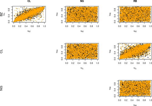
Figures 8 and 9 show the scatterplots of the pseudo-observations obtained via non parametric estimation of the marginals in Period 1 and 2, respectively. For a visual comparison between the observations and the fitted models, we have simulated new pseudo-data from the estimated models and plotted together with the original data. It is evident that CL and BZ show the strongest dependence, while RB shows an average level of dependence with both CL and BZ. As expected, NG has the lowest level of dependence with all the other assets. Moreover, the scatterplots show a visual change in the dependence structure, where assets in Period 1 seem to be more strongly dependent than in Period 2. Finally, the comparison with the simulated pesudo-observations (in orange in the plots) seem to support the choice of the models.

Fig. 8 Dependence scatterplots for pseudo-observations (black) and observations simulated from the fitted models (orange) in Period 1.

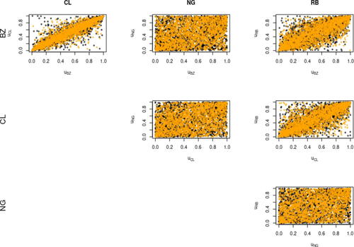
Fig. 9 Dependence scatterplots for pseudo-observations (black) and observations simulated from the fitted models (orange) in Period 2.

5 Discussion

We examined the dependence structure of crude oil prices in periods of irregular and regular OPEC announcements. We performed an analysis to check the best copula model to represent co-movements between crude oil benchmark prices and their derivatives. We found evidence of symmetric tail dependence, captured by a Student-t copula for Brent crude oil and WTI crude oil, Brent crude oil and gasoline RB and WTI crude oil and gasoline RB. We saw a consistent decreasing of the dependence among asset prices in periods of regular OPEC announcements, regarding both the overall dependence (investigated through the Spearman’s ρ_S and the Kendall’s τ) and the tail dependence. In particular, our analysis showed that natural gas prices, which are generally less influenced by crude oil prices, show a dependence close to zero with the other asset prices we investigated in this work in the period of regular announcements.

To the best of our knowledge, this analysis is novel in the literature: in times of crude oil markets stress, the co-movements of crude oil prices and derivatives are more strongly related; on the other hand, in periods of stable global demand of crude oil, OPEC decreases the number of extraordinary meetings and the dependence structure among crude oil and derivatives’ prices is reduced. Interestingly, the only case where the level of tail dependence increases from the first to the second period is the pair of Brent crude oil and gasoline RB; while in all other combinations, tail dependence decreases. The proposed methodology has the important advantage to realistically model each asset price series separately, avoiding the need to implement simplistic joint distributions. Moreover, several assumptions on the type of the dependence can be tested and the best model for the co-movements can be chosen. While we do not aim at establishing a causal relationship between the regularity of the OPEC announcements and the strenght of the dependence, we think that the findings have important implications for risk management: in period of stress, tail dependence tends to be higher, that is, joint losses in crude oil markets are more likely; on the other hand, it tends to decrease in periods where OPEC does not need to adjust prices through output.

Acknowledgements

This research did not receive any specific grant from funding agencies in the public, commercial, or not-for-profit sectors.

References

- Aielli, G. P. (2013). Dynamic conditional correlation: On properties and estimation. Journal of Business & Economic Statistics 31(3):282–299. doi:10.1080/07350015.2013.771027
- Ané, T., Kharoubi, C. (2003). Dependence structure and risk measure*. The Journal of Business 76(3):411–438. doi:10.1086/375253
- Azam, K., (2014). Effects of marginal specifcations on copula estimation. Technical report.
- Azzalini, A., Capitanio, A. (2003). Distributions generated by perturbation of symmetry with emphasis on a multivariate skew t-distribution. Journal of the Royal Statistical Society Series B: Statistical Methodology 65(2):367–389. doi:10.1111/1467-9868.00391
- Bakirov, N. K., Rizzo, M. L., Székely, G. J. (2006). A multivariate nonparametric test of independence. Journal of Multivariate Analysis 97(8):1742–1756. doi:10.1016/j.jmva.2005.10.005
- Caporin, M., McAleer, M. (2014). Robust ranking of multivariate GARCH models by problem dimension. Computational Statistics & Data Analysis 76:172–185. doi:10.1016/j.csda.2012.05.012
- Chan, K. F., Treepongkaruna, S., Brooks, R., Gray, S. (2011). Asset market linkages: Evidence from financial, commodity and real estate assets. Journal of Banking & Finance 35(6):1415–1426. doi:10.1016/j.jbankfin.2010.10.022
- Cherubini, U., Luciano, E., Vecchiato, W. (2004). Copula Methods in Finance. John Wiley & Sons.
- Darbellay, G. A., Vajda, I. (2000). Entropy expressions for multivariate continuous distributions. IEEE Transactions on Information Theory 46(2):709–712. doi:10.1109/18.825848
- De Lira Salvatierra, I., Patton, A. J. (2015). Dynamic copula models and high frequency data. Journal of Empirical Finance 30:120–135. doi:10.1016/j.jempfin.2014.11.008
- Deaves, R., Krinsky, I. (1992). The behavior of oil futures returns around OPEC conferences. Journal of Futures Markets 12(5):563–574. doi:10.1002/fut.3990120507
- Demirer, R., Kutan, A. M. (2010). The behavior of crude oil spot and futures prices around OPEC AND SPR announcements: An event study perspective. Energy Economics 32(6):1467–1476. doi:10.1016/j.eneco.2010.06.006
- Draper, D. W. (1984). The behavior of event-related returns on oil futures contracts. Journal of Futures Markets 4(2):125–132. doi:10.1002/fut.3990040203
- Ebrahimi, N., Jalali, N. Y., Soofi, E. S. (2014). Comparison, utility, and partition of dependence under absolutely continuous and singular distributions. Journal of Multivariate Analysis 131:32–50. doi:10.1016/j.jmva.2014.06.014
- Embrechts, P., Lindskog, F., Mcneil, A. (2001). Modelling dependence with copulas. Rapport technique, Département de mathématiques, Institut Fédéral de Technologie de Zurich, Zurich 14:1–50.
- Embrechts, P., Mcneil, A., Straumann, D. (2002). Correlation and dependence in risk management: Properties and pitfalls. In M. A. H. Dempster, ed., Risk Management: Value at Risk and Beyond, vol. 1, Cambridge: Cambridge University Press, pp. 176–223.
- Engle, R. F. (1982). Autoregressive conditional heteroscedasticity with estimates of the variance of united kingdom inflation. Econometrica 50(4):987. doi:10.2307/1912773
- Fang, H.-B., Fang, K.-T., Kotz, S. (2002). The meta-elliptical distributions with given marginals. Journal of Multivariate Analysis 82(1):1–16. doi:10.1006/jmva.2001.2017
- Fantazzini, D. (2009). The effects of misspecified marginals and copulas on computing the value at risk: A monte carlo study. Computational Statistics & Data Analysis 53(6):2168–2188. doi:10.1016/j.csda.2008.02.002
- Fattouh, B., (2005). The causes of crude oil price volatility. Middle East Economic Survey XLVIII(13).
- Francq, C., Zakoian, J.-M. (2004). Maximum likelihood estimation of pure GARCH and ARMA-GARCH processes. Bernoulli 10(4):605–637. 10.3150/bj/1093265632
- Geenens, G., Lafaye de Micheaux, L. P. (2020). The hellinger correlation. Journal of the American Statistical Association 1–15. 10.1080/01621459.2020.1791132
- Genest, C., Ghoudi, K., Rivest, L.-P. (1995). A semiparametric estimation procedure of dependence parameters in multivariate families of distributions. Biometrika 82(3):543–552. doi:10.1093/biomet/82.3.543
- Genest, C., Werker, B. J. (2002). Conditions for the asymptotic semiparametric efficiency of an omnibus estimator of dependence parameters in copula models. In Distributions with given Marginals and Statistical Modelling. Springer, pp. 103–112.
- Geweke, J. (1993). Bayesian treatment of the independent student-t linear model. Journal of Applied Econometrics 8(S1): 19–40. 10.1002/jae.3950080504
- Granger, C., Lin, J.-L. (1994). Using the mutual information coefficient to identfy LAGS in nonlinear models. Journal of Time Series Analysis 15(4):371–384. doi:10.1111/j.1467-9892.1994.tb00200.x
- Granger, C. W., Maasoumi, E., Racine, J. (2004). A dependence metric for possibly nonlinear processes. Journal of Time Series Analysis 25(5):649–669. doi:10.1111/j.1467-9892.2004.01866.x
- Grazian, C., Liseo, B. (2017). Approximate bayesian inference in semiparametric copula models. Bayesian Analysis 12(4):991–1016. 10.1214/17-BA1080
- Guidi, M. G., Russell, A., Tarbert, H. (2006). The effect of OPEC policy decisions on oil and stock prices. OPEC Review 30(1):1–18. doi:10.1111/j.1468-0076.2006.00157.x
- Ji, Q., Liu, B.-Y., Nehler, H., Uddin, G. S. (2018). Uncertainties and extreme risk spillover in the energy markets: A time-varying copula-based covar approach. Energy Economics 76:115–126. doi:10.1016/j.eneco.2018.10.010
- Jiang, Z.-Q., Xie, W.-J., Zhou, W.-X. (2014). Testing the weak-form efficiency of the WTI crude oil futures market. Physica A: Statistical Mechanics and Its Applications 405:235–244. doi:10.1016/j.physa.2014.02.042
- Joe, H. (2005). Asymptotic efficiency of the two-stage estimation method for copula-based models. Journal of Multivariate Analysis 94(2):401–419. doi:10.1016/j.jmva.2004.06.003
- Joo, K., Suh, J. H., Lee, D., Ahn, K. (2020). Impact of the global financial crisis on the crude oil market. Energy Strategy Reviews 30:100516 doi:10.1016/j.esr.2020.100516
- Kaufmann, R. K., Dees, S., Karadeloglou, P., Sanchez, M. (2004). Does OPEC matter? An econometric analysis of oil prices. The Energy Journal 25:4. 10.5547/ISSN0195-6574-EJ-Vol25-No4-4
- Kim, G., Silvapulle, M. J., Silvapulle, P. (2007). Comparison of semiparametric and parametric methods for estimating copulas. Computational Statistics & Data Analysis 51(6):2836–2850. doi:10.1016/j.csda.2006.10.009
- Klein, T. (2018). Trends and contagion in WTI AND brent crude oil spot and futures markets- THE role of OPEC in the last decade. Energy Economics 75:636–646. doi:10.1016/j.eneco.2018.09.013
- Koirala, K. H., Mishra, A. K., D’Antoni, J. M., Mehlhorn, J. E. (2015). Energy prices and agricultural commodity prices: Testing correlation using copulas method. Energy 81:430–436. doi:10.1016/j.energy.2014.12.055
- Liu, P., Vedenov, D., Power, G. J. (2020). Commodity financialization and sector etfs: Evidence from crude oil futures. Research in International Business and Finance 51:101109. doi:10.1016/j.ribaf.2019.101109
- Ljung, G. M., Box, G. E. P. (1978). On a measure of lack of fit in time series models. Biometrika 65(2):297–303. doi:10.1093/biomet/65.2.297
- Loutia, A., Mellios, C., Andriosopoulos, K. (2016). Do OPEC announcements influence oil prices?. Energy Policy 90:262–272. doi:10.1016/j.enpol.2015.11.025
- Lu, X. F., Lai, K. K., Liang, L. (2014). Portfolio value-at-risk estimation in energy futures markets with time-varying copula-GARCH model. Annals of Operations Research 219(1):333–357. doi:10.1007/s10479-011-0900-9
- MacKenzie, D., Spears, T. (2014). The formula that killed wall street’: The Gaussian copula and modelling practices in investment banking. Social Studies of Science 44(3):393–417. doi:10.1177/030631271351715725051588
- Malevergne, Y., Sornette, D. (2003). Testing the gaussian copula hypothesis for financial assets dependences. Quantitative Finance 3(4):231–250. doi:10.1088/1469-7688/3/4/301
- Martina, E., Rodriguez, E., Escarela-Perez, R., Alvarez-Ramirez, J. (2011). Multiscale entropy analysis of crude oil price dynamics. Energy Economics 33(5):936–947. doi:10.1016/j.eneco.2011.03.012
- Mohammadi, H., Su, L. (2010). International evidence on crude oil price dynamics: Applications of ARIMA-GARCH models. Energy Economics 32(5):1001–1008. doi:10.1016/j.eneco.2010.04.009
- Nadarajah, S., Zografos, K. (2005). Expressions for rényi and shannon entropies for bivariate distributions. Information Sciences 170(2-4):173–189. doi:10.1016/j.ins.2004.02.020
- Nikoloulopoulos, A. K., Karlis, D. (2008). Copula model evaluation based on parametric bootstrap. Computational Statistics & Data Analysis 52(7):3342–3353. doi:10.1016/j.csda.2007.10.028
- Ning, C. (2010). Dependence structure between the equity market and the foreign exchange market–a copula approach. Journal of International Money and Finance 29(5):743–759. doi:10.1016/j.jimonfin.2009.12.002
- OPEC Secretariat. (2003). OPEC production agreements: A detailed listing. OPEC Review 27(1):65–77. doi:10.1111/1468-0076.00124
- Patton, A. J. (2004). On the out-of-sample importance of skewness and asymmetric dependence for asset allocation. Journal of Financial Econometrics 2(1):130–168. doi:10.1093/jjfinec/nbh006
- Patton, A. J. (2006). Modelling asymmetric exchange rate dependence*. International Economic Review 47(2):527–556. doi:10.1111/j.1468-2354.2006.00387.x
- Patton, A. J. (2012). A review of copula models for economic time series. Journal of Multivariate Analysis 110:4–18. doi:10.1016/j.jmva.2012.02.021
- Reboredo, J. C. (2011). How do crude oil prices co-move?. Energy Economics 33(5):948–955. doi: 10.1016/j.eneco.2011.04.006
- Salisu, A. A. (2016). Modelling oil price volatility with the beta-skew-t-EGARCH framework. Economics Bulletin 36(3):1315–1324.
- Schloegl, L., O’Kane, D. (2005). A note on the large homogeneous portfolio approximation with the student-t copula. Finance and Stochastics 9(4):577–584. doi:10.1007/s00780-004-0142-7
- Schmid, F., Schmidt, R. (2007). Multivariate extensions of spearman’s rho and related statistics. Statistics & Probability Letters 77(4):407–416. doi:10.1016/j.spl.2006.08.007
- Sklar, A. (1959). Fonctions de répartition à n dimensions et leurs marges. Publications de l’, Institut Statistique de l’Université de Paris 8:229–231.
- Székely, G. J., Rizzo, M. L., Bakirov, N. K. (2007). Measuring and testing dependence by correlation of distances. The Annals of Statistics 35(6):2769–2794. 10.1214/009053607000000505
- Teräsvirta, T., (2009). An introduction to univariate GARCH models. In Handbook of Financial Time Series, 1st ed. Berlin: Springer, pp. 17–42.
- U. S.Energy Information Administration. (2021-07-17). Natural Gas-Henry Hub Natural Gas Spot Price.
- U.S. Energy Information Administration. (2021). Petroleum & Other Liquids-Cushing, OK WTI Spot Price FOB-Dollars Per Barrel. Available at https://www.eia.gov/dnav/pet/hist/LeafHandler.ashx?n=PET&s=RWTC&f=M. Last accessed 17 July 2021.
- Vogiatzoglou, M. (2021). Dynamic copula toolbox 3.0. In MATLAB Central File Exchange.
- Wirl, F., Kujundzic, A. (1984). The impact of OPEC conference outcomes on world oil prices. The Energy Journal (1):25. 10.5547/ISSN0195-6574-EJ-Vol25-No1-3
- Zhang, Y.-J., Chevallier, J., Guesmi, K. (2017). De-financialization” of commodities? Evidence from stock, crude oil and natural gas markets. Energy Economics 68:228–239. doi:10.1016/j.eneco.2017.09.024