Groundwater geochemistry, hydrogeology and potash mineral potential of the Lake Woods region, Northern Territory, Australia

Abstract

We collected 38 groundwater and two surface-water samples in the semi-arid Lake Woods region of the Northern Territory to better understand the hydrogeochemistry of this system, which straddles the Wiso, Tennant Creek and Georgina geological regions. Lake Woods is presently a losing waterbody feeding the underlying groundwater system. The main aquifers comprise mainly carbonate (limestone and dolostone), siliciclastic (sandstone and siltstone) and evaporitic units. The water composition was determined in terms of bulk properties (pH, electrical conductivity, temperature, dissolved oxygen, redox potential), 40 major, minor and trace elements, and six isotopes (δ¹⁸O_water, δ²H_water, δ¹³C_DIC, δ³⁴S_SO4^2–, δ¹⁸O_SO4^2–, ⁸⁷Sr/⁸⁶Sr). The groundwater is recharged through infiltration in the catchment from monsoonal rainfall (annual average rainfall ∼600 mm) and runoff. It evolves geochemically mainly through evapotranspiration and water–mineral interaction (dissolution of carbonates, silicates and to a lesser extent sulfates). The two surface waters (one from the main creek feeding the lake, the other from the lake itself) are extraordinarily enriched in ¹⁸O and ²H isotopes (δ¹⁸O of +10.9 and +16.4‰ VSMOW, and δ²H of +41 and +93‰ VSMOW, respectively), which is interpreted to reflect evaporation during the dry season (annual average evaporation ∼3000 mm) under low humidity conditions (annual average relative humidity ∼40%). This interpretation is supported by modelling results. The potassium (K) relative enrichment (K/Cl^– mass ratio over 50 times that of sea water) is similar to that observed in salt-lake systems worldwide that are prospective for potash resources. Potassium enrichment is believed to derive partly from dust during atmospheric transport/deposition, but mostly from weathering of K-silicates in the aquifer materials (and possibly underlying formations). Further studies of Australian salt-lake systems are required to reach evidence-based conclusions on their mineral potential for potash, lithium, boron and other low-temperature mineral system commodities such as uranium.

Keywords:

• Groundwater
• hydrogeochemistry
• mineral systems
• potash
• processes
• Australia

Introduction

Despite the large number of salt lakes distributed across Australia, knowledge of saline lakes and their associated groundwater systems as potential resources of potash and other commodities is limited [the term ‘potash’ denotes a variety of salts of potassium (K), such as K chloride, carbonate and sulfate; Jasinski, 2015]. Mernagh et al. (2013) reviewed publicly available national-scale datasets on Australian saline lakes and developed mineral systems models, which were then used to assess the potential of these salt-lake systems for potash and other low-temperature mineral commodities at that scale. That review, later summarised in Mernagh et al. (2016), noted that the Lake Woods region in the Northern Territory has elevated concentrations of K in bore waters that have a spatial association with outcropping rocks containing evaporitic units, mostly within the Tennant Creek geological region (their figure 7). The review recommended further studies be carried out to assess the potential for economic concentrations of potash (as well as lithium (Li) and boron (B)) in this region.

In Australia, no in-depth study of salt-lake systems with a view to determine their mineral potential in terms of Li B and K resources have been published in the publicly available scientific literature. Lake Woods has not previously been investigated in terms of the occurrence of solute-rich groundwaters or the relationship between such groundwaters and seasonal lake waters. However, it was known that regionally the Lake Woods area shows relative K-enrichment values comparable with those reported for groundwaters associated with economic salt-lake potash deposits on other continents (Mernagh et al., 2013, and references therein). Moreover, the relationship between lake hydrological processes and geomorphological evolution has not been explored at Lake Woods to any extent compared with some Australian salt lakes (for instance: Lake Tyrrell, e.g. Bowler & Teller, 1986; Lake Eyre, e.g. Magee & Miller, 1998). Accordingly, the present study included field and analytical investigations at Lake Woods in order to enhance our understanding of a little-known ephemeral lake in a remote part of the continent and to compare our results with better-understood salt-lake systems (e.g. Lake Tyrrell, Lake Eyre). It is worth noting as well that mineral, energy and groundwater resources are the focus of ‘Exploring for the Future,’ a 2016–2020 Australian government research and development initiative aimed at boosting exploration investment in Australia’s resources sector, particularly in northern Australia (DIIS, 2016).

Physiographic and geological setting

Lake Woods [17.84°S, 133.52°E, elevation 198 m Australian Height Datum (AHD)] is a large ephemeral lake located near the township of Elliott, in the semi-arid zone of the Northern Territory (Figure 1). The lake lies to the west of the Stuart Highway that links Darwin and Alice Springs, ∼650 km SSE of Darwin (Figure 1a). It is at the western edge of the Barkly Tableland, a vast inland plain that extends across adjoining expanses of the Northern Territory and Queensland, and is characterised by endorheic drainage. The lake is surrounded by eolian sand sheets and dunes of the Tanami Desert to the west and south. Lake Woods covers an area of up to ∼500 km², although it is sometimes dry. The lake catchment is approximately 25 300 km² in extent (Bowler, Duller, Perret, Prescott, & Wyrwoll, 1998) and includes black soil and laterite plains, dunefields and bedrock hills. Annual average climate conditions at the Elliott weather station (17.56°S, 133.54°E, elevation 220 m AHD), some 14 km to the north of the lake, are characteristic of a semi-arid climate: rainfall ∼600 mm (falling almost entirely during summer, November to March), potential evaporation ∼3000 mm, and relative humidity 30–60% (BOM, 2016). During the wet monsoonal season, winds recorded at the Tindal weather station (some 375 km to the NNW of Lake Woods) are dominantly from the northwest (BOM, 2017). The Supplementary papers (Figure S1) show the wider study area on a Digital Elevation Model and satellite imagery, for reference.

Figure 1. (a) Location of the sampled sites within the Lake Woods area, Northern Territory, Australia, overlain on a satellite image (Esri, 2016) and (b) on a geological map (Raymond, Liu, Gallagher, Zhang, & Highet, 2012). Also shown are (a) major geomorphic features, and (b) Wiso, Tennant Creek, and Georgina geological region boundaries (bold dark grey lines; Blake & Kilgour, 1998). The symbol colours represent the four quartiles of (a) total dissolved solids (TDS, in mg/L) and (b) dissolved potassium concentration (K, in mg/L); the circles are groundwater samples, the triangles are surface water samples (see text). The inset map shows the location of the study area in Australia (square) and of three rain water sample sites (crosses; from W to E: Halls Creek, Alice Springs, Mount Isa; Crosbie et al., 2012; see text).

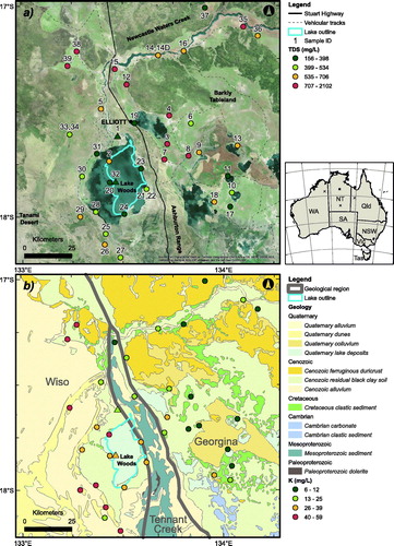
The regional geology (Figure 1b) comprises the Paleozoic Wiso and Neoproterozoic to Paleozoic Georgina geological regions (Blake & Kilgour, 1998) in the west and east of the study area, respectively, as well as a central sliver of the Paleoproterozoic to Mesoproterozoic Tennant Creek geological region. The corresponding geological/geomorphological entities are the Wiso and Georgina basins in the west and east, separated by the north–south-striking bedrock ridge of the Ashburton Range. The ridge rises up to 90 m above the surrounding sandy plains to an altitude of ∼360 m AHD. Lake Woods lies against the western flank of the Ashburton Range, mostly overlying the Wiso Basin and the southern edge of the Cretaceous Carpentaria Basin. Paleolake extent, however, indicates that Lake Woods once lapped east of the Ashburton Range in addition to large extensions to the west of the present-day lake outline (Bowler et al., 1998). The catchment thus includes several major geological provinces (Stewart, Raymond, Totterdell, Zhang, & Gallagher, 2013): the Tomkinson Province making up the Ashburton Range, as well as the Wiso, Georgina and Carpentaria basins. Structurally, the folded and faulted Proterozoic units contrast with the flat-lying to gently dipping Cambrian rocks. The stratigraphy of the area is summarised in Table 1 and is discussed further in the Supplementary Papers.

Table 1. Generalised stratigraphy of the Lake Woods region.

Formation	Age	Geological region	Maximum thickness	Significant aquifer	Description
Brunette Limestone	Cenozoic (11.5 Ma)	NA	18 m		Fossiliferous nodular white limestone, silicified in part and containing chert nodules and bands, minor quartz sandstone and conglomerate; characteristic features include rhizoliths, Cambrian pebbles, alveolar texture, circum- and intragranular cracks
Tertiary Laterite	Cenozoic	NA	6 m		Laterite, ferruginous rubble, some soil cover
Mullaman beds	Cretaceous (Aptian)	Carpentaria	NA		Quartz sandstone and conglomerate, sandy claystone and siltstone
Anthony Lagoon Formation	Middle Cambrian	Georgina	NA	Yes; porous to karstic; depth 35–145 m below surface; regional flow direction NW; yield 0.5–25 L/s; recharge mainly through seasonal infiltration from, e.g. Lake Tarrabool and throughflow from the Gum Ridge Formation in the W	Dolomudstone/dolosparstone, dolomitic-siliciclastic siltstone and mudstone, dolomitic sandstone–siltstone interbeds; evaporites (mostly gypsum), chert concretions; minor intraclast and oncoid dolostone, microbial dololaminite, dolomitic quartz sandstone; equivalent to Point Wakefield beds (Wiso)
Point Wakefield beds	Middle Cambrian	Wiso	54 m	See Anthony Lagoon Formation (Georgina)	Brown and white claystone; red to white, fine, angular well sorted marine sandstone, laminated red-brown and white micaceous siltstone and claystone; minor local conglomerate; bioturbated, fossiliferous; equivalent to Anthony Lagoon Formation (Georgina)
Lothari Hill Sandstone	Middle Cambrian	Wiso	94 m		Red-brown laminated claystone; white fine-grained angular sandstone; tidal deposits
Hooker Creek Formation	Middle Cambrian	Wiso	162 m		Red, laminated, bioturbated, micaceous dolomitic siltstone, sandstone; white, finely crystalline dolomite with algal structures in part; red-brown colour in outcrop probably owing to weathering
Gum Ridge Formation	Middle Cambrian	Georgina	151 m	Yes; porous to karstic; depth 15–168 m below surface; regional flow direction E–NE; yield 0.5–25 L/s; recharge mainly through seasonal creek infiltration; discharge mainly into Anthony Lagoon beds	Grey, partially dolomitised massive, ribbon, bioclast, lithoclast and minor onkoid limestone, minor cryptomicrobial dololaminite and grey siliciclastic mudstone; brown-maroon siltstone at base; recessive outcrop pervasively chertified and lateritised; lateral correlative of Montejinni Limestone (Wiso)
Montejinni Limestone	Middle Cambrian (Early Templetonian)	Wiso	1512 m	Yes; porous to karstic; SWL 24–49 m below surface; regional flow direction W–NW; yield 0.5–25 L/s; recharge mainly through seasonal infiltration from Lake Woods	Fossiliferous limestone, dolostone, calcareous mudstone; minor fine-grained sandstone and siliciclastic mudstone; chert and nodular evaporitic pseudomorphs; silicified outcrop, recessive; lateral correlative of Gum Ridge Formation (Georgina)
Helen Spring Volcanics	Early–Middle Cambrian (511–508 Ma)	Wiso, Tennant	36 m	Partly; not a major aquifer in the Wiso; porous to fractured aquifer in Tennant geological region; depth 2–64 m below surface; yield 0.5–5 L/s	Weathered vesicular basalt; minor trachyte, microdolerite; minor dolerite; volcaniclastic rocks; basal pebbly mudstone, conglomerate and lithic arenite
Antrim Plateau Volcanics	Early–Middle Cambrian (513–505 Ma)	Wiso	1500 m		Massive and amygdaloidal tholeiitic basalt and basalt breccia; commonly capped by ferricrete; agglomerate with brecciated flow tops; minor sandstone and chert interbeds
Renner Group	Mesoproterozoic (1492–1429 Ma)	Tennant	3500 m		Quartz arenite, sublithic arenite, siltstone; minor mudstone and conglomerate; halite pseudomorphs
Namerinni Group	Paleoproterozoic (1660–1610 Ma)	Tennant	2800 m		Quartz arenite, sublithic/lithic arenite, dolostone, mudstone; minor conglomerate; evaporite pseudomorphs locally abundant; stromatolites
Tomkinson Creek Group	Paleoproterozoic (1805–1710 Ma)	Tennant	NA	Partly; fractured; depth 2–140 m; yield 0.1–0.5 L/s	A thick succession of shallow-marine and continental sedimentary rocks, with minor mafic volcanic rocks in the lower part

Sources: ASUD (2016); Blake and Kilgour (1998); Verma and Jolly (1992). Note: SWL: Standing Water Level.

Hydrogeological setting

Lake Woods typically occupies an area of 350–500 km², although during periods of major flooding it can extend to 850 km² and, at times, nearer 1000 km², making it one of the largest ephemeral lakes in the Northern Territory (e.g. see satellite image in Figure 1a). The lake is fed by freshwater dominantly by Newcastle Waters Creek that drains from the northeast, and passes through an erosional gap in the Ashburton Range ∼30 km north of Elliott (see Figure 1a). This creek, which hydrographs indicate to be regularly flooding by several metres at the end of the wet season, drains an area of approximately 19,000 km² of the Barkly Tableland (Georgina geological region) to the east of the Ashburton Range. Some local runoff is received from numerous minor drainage lines on the western flank of the Ashburton Range, although such drainage typically terminates in alluvial floodouts at the base of the range, possibly flowing beneath sand plains rather than maintaining creek lines directly to the lake. Although Lake Woods appears to be a terminal drainage system, it is underlain by low salinity aquifers and is a groundwater recharging system. The depth to groundwater in the Lake Woods area ranges mostly from 15 to 90 m below the ground surface (Tickell, 2003; Verma & Jolly, 1992). Further details pertaining to the hydrogeological environment of the Lake Woods region are given in the Supplementary Papers.

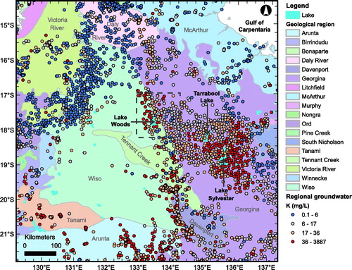
Extensive regional groundwater analyses carried out by the Northern Territory Department of Environment and Natural Resources (Tickell, 2003) indicate that Lake Woods sits at the western end of a region characterised by groundwater that contains elevated K concentrations (Figure 2). This region extends across the Georgina Basin, with the highest concentrations occurring near Lake Sylvester and Tarrabool Lake, some 170–250 km ESE of Lake Woods, and along the western edge of the Georgina and Davenport geological regions, including in the vicinity of Lake Woods. Supplementary papers (Figure S2) show the K/Cl ratio map for the same region.

Figure 2. Regional groundwater bore distribution in the central Northern Territory (S. Tickell, pers comm, 2014) overlain on geological regions (Blake & Kilgour, 1998). The symbol colours represent the four quartiles of dissolved potassium concentration (K, in mg/L). The dashed box shows the location of the Lake Woods study area. Lake Sylvester and Tarrabool Lake, mentioned in the text, are also shown.

Groundwaters in local carbonate rock aquifers are primarily recharged by infiltration of water from overlying creeks and lakes rather than directly by rainfall infiltration or runoff from ranges (Verma & Jolly, 1992). Thus, in the scheme of Winter, Harvey, Franke, and Alley (1998), lakes Woods, Tarrabool and Sylvester and other small seasonal lakes are ‘losing waterbodies’ whereby lake water is lost to the underlying groundwater system rather than being recharged by it. In comparison, in more arid parts of Australia, the opposite is usual, with groundwaters typically discharging to salt lakes. In the Georgina Basin, this recharge mechanism, with lake water infiltrating underlying aquifers, applies to the Gum Ridge and Anthony Lagoon formations. The Anthony Lagoon Formation aquifer additionally receives groundwater via throughflow from the underlying Gum Ridge Formation (Verma & Jolly, 1992). In the Wiso Basin, Lake Woods recharges the underlying Cambrian Montejinni Limestone, and this recharge is more significant than intake waters received by the aquifer from direct rainfall infiltration and runoff from the Ashburton Range. Groundwater flow is towards the northwest (Verma & Jolly, 1992), most likely into the equivalent Cambrian Tindall Limestone aquifer of the Daly Basin (Knapton, 2006).

Methods

Thirty-eight groundwater samples (including three field duplicate samples) were collected from 35 pastoral bores around Lake Woods from late August to mid-September 2013 (i.e. relatively late in the dry season). In addition, two surface-water samples were collected, one from the Newcastle Waters Creek and the other from Lake Woods itself. Sampling sites are shown in Figure 1. In the assessment of analytical results (Results and Discussion), we compare the new water data to average sea water (Drever, 1997) and to the 2007–2011 amount-weighted average rain-water composition from three regional sites: Alice Springs, Halls Creek and Mount Isa (see Figure 1 inset for location; Crosbie et al., 2012). The latter comparison is particularly relevant in light of the hydrogeological conditions of the study area, which are characterised by a groundwater-feeding lake system, implying the need to interpret the geochemistry along the rain water-to-surface water-to-groundwater evolutionary pathway.

In the field, the following parameters were monitored and measured using a flow cell, where possible, to minimise contact with the atmosphere: water pH, specific electrical conductivity compensated to 25°C (EC), temperature (T), redox potential (Eh) and dissolved oxygen (DO). Total alkalinity was also determined on site from freshly collected water as mg/L CaCO₃ and converted to mg/L HCO₃^– for data analysis. Field equipment was calibrated daily prior to sampling. Additionally, at each site, quality control checks were undertaken to ensure proper functioning of the equipment. Pumped bores were monitored for stabilised parameters (especially pH, T and EC) prior to sampling to ensure fresh groundwater was being collected as opposed to stagnant bore water, which could be contaminated by fallen debris, interaction with bore/pump materials and the atmosphere, or rain/flood water ingress. Two surface-water samples, one from Newcastle Waters Creek, the other from Lake Woods itself, were collected as grab samples a few centimetres under the water surface and without disturbing bottom sediments. Details of field equipment and procedures are reported in the Supplementary papers (Table S1).

Several aliquots of water were collected at each site for various analyses and the following sample preparation protocols were carried out in the field. Where filtration was required, Millipore mixed cellulose 0.45 µm filters were used, either inline or via a pressure vessel and Millipore Swinnex filter holder. Filters were changed for each site. Where the sample was turbid and difficult to filter, Millipore glass fibre pre-filters were used upstream of the 0.45 µm filter. At Site LW32, the lake water was very turbid and filtered through a high capacity 0.45 µm Waterra inline filter. The aliquot for anion analysis was filtered directly into a 30 mL Sarstedt polypropylene (PP) bottle and refrigerated. The aliquot for cation analysis was filtered directly into a 30 mL Sarstedt PP bottle, acidified with concentrated ultrapure HNO₃ to 2% v/v, and refrigerated.

Duplicate samples for oxygen and hydrogen isotope analysis were collected raw (unfiltered and untreated) in two 10 mL additive-free, sterile plastic Vacutainer tubes. The aliquot for carbon isotopic analysis of dissolved inorganic carbon (DIC) was filtered through a 0.45 µm filter as described above into a 500 mL Cospak-supplied low density polyethylene (LDPE) bottle, alkalinised with concentrated NaOH and treated with SrCl₂ powder to induce precipitation of DIC as SrCO₃. The aliquot for sulfur isotopic analysis of dissolved sulfate was filtered into a 500 mL Cospak-supplied LDPE bottle, acidified with concentrated HCl and treated with BaCl₂ powder to induce precipitation of dissolved sulfate as BaSO₄. The aliquot for strontium isotopic analysis was collected as per the aliquot for cation analysis (i.e. filtered and acidified).

All samples, apart from carbon and sulfur isotope precipitates, were stored refrigerated for the length of the field trip and subsequently transported in insulated cool boxes with ice bricks via refrigerated freight to the Geoscience Australia laboratories in Canberra, Australia.

Details on the laboratory analytical methods and quality control/quality assessment procedures are given in the Supplementary papers.

Results and discussion

Surface and groundwater geochemistry

All geochemical data are summarised in Table 2; the full dataset (which consists of site metadata; five field-determined bulk properties pH, EC, T, Eh and DO; 40 anion and cation concentrations; and six isotope ratios) is available in the Supplementary papers (Table S2).

Table 2. Statistical summary of hydrogeochemical data for the water samples from Lake Woods.

Parameter	Units	Method	LLD	Min	Med	Ave	Max	Surface water (creek)	Surface water (lake)
Field parameters
T	°C	Field probe	NA	21.2	30.3	29.0	38.7	31.5	27.5
EC	µS/cm	Field probe	10	354	922	1040	3150	324	486
DO	mg/L	Field probe	0.1	<0.1	2.7	2.7	6.6	3.4	5.6
pH	NA	Field probe	NA	5.64	6.96	6.97	7.59	6.89	8.94
Eh	mV	Field probe	NA	78	236	239	399	395	108
Major cations
Na	mg/L	ICP-OES	0.3	8.3	83.3	91.8	391.0	7.1	20.7
K	mg/L	ICP-OES	0.5	5.9	23.6	26.6	58.7	14.4	28.8
Ca	mg/L	ICP-OES	0.1	13.1	65.2	70.1	162.0	27.2	46.3
Mg	mg/L	ICP-OES	0.1	10.8	41.7	40.6	96.5	14.2	7.9
Major anions
Cl^–	mg/L	IC	2	7.8	51.4	115.7	598.0	15.1	53.8
HCO3^–	mg/L	Titration	10	70.8	433.7	422.2	658.8	159.8	162.3
SO4^2–	mg/L	IC	0.5	2.6	64.3	102.1	639.2	6.0	21.3
Br^–	mg/L	IC	0.025	0.07	0.27	0.62	2.74	0.09	0.44
F^–	mg/L	IC	0.02	0.15	1.07	1.24	3.30	0.19	0.61
Trace elements
Al	mg/L	ICP-MS	0.0001	0.0008	0.0027	0.0039	0.0174	0.0019	0.0121
As	mg/L	ICP-MS	0.0001	0.0002	0.0012	0.0032	0.0712	0.0019	0.0194
B	mg/L	ICP-OES	0.01	0.06	0.24	0.28	0.99	0.12	0.35
Ba	mg/L	ICP-MS	0.005	0.025	0.100	0.183	0.590	0.179	0.157
Co	mg/L	ICP-MS	0.0001	<0.0001	<0.0001	0.0002	0.0042	0.0004	0.0002
Cr	mg/L	ICP-MS	0.0001	<0.0001	0.0004	0.0006	0.0020	0.0005	<0.0001
Cs	mg/L	ICP-MS	0.0001	<0.0001	<0.0001	0.0001	0.0012	<0.0001	<0.0001
Cu	mg/L	ICP-MS	0.0001	0.0004	0.0019	0.0075	0.0487	0.0042	0.0037
Eu	mg/L	ICP-MS	0.0001	<0.0001	<0.0001	<0.0001	0.0002	<0.0001	<0.0001
Fe	mg/L	ICP-MS	0.0001	<0.0001	<0.0001	0.3538	10.1093	<0.0001	0.0032
Ga	mg/L	ICP-MS	0.0001	0.0004	0.0026	0.0048	0.0162	0.0048	0.0043
Ge	mg/L	ICP-MS	0.0001	<0.0001	0.0002	0.0003	0.0021	<0.0001	<0.0001
Hf	mg/L	ICP-MS	0.0001	<0.0001	<0.0001	<0.0001	0.0004	0.0002	<0.0001
Li	mg/L	ICP-MS	0.0001	0.0011	0.0284	0.0339	0.1334	0.0003	0.0002
Mn	mg/L	ICP-MS	0.0001	<0.0001	0.0007	0.0262	0.3109	0.0017	0.0060
Mo	mg/L	ICP-MS	0.0001	<0.0001	0.0018	0.0027	0.0162	0.0006	0.0028
Ni	mg/L	ICP-MS	0.0001	<0.0001	<0.0001	0.0003	0.0040	0.0005	0.0017
P	mg/L	ICP-MS	0.0001	<0.0001	0.0035	0.0066	0.0542	0.0219	0.0528
Pb	mg/L	ICP-MS	0.0001	<0.0001	<0.0001	0.0001	0.0010	<0.0001	<0.0001
Rb	mg/L	ICP-MS	0.0001	0.0060	0.0155	0.0167	0.0304	0.0213	0.0102
Sc	mg/L	ICP-MS	0.0001	<0.0001	0.0101	0.0106	0.0181	0.0036	0.0142
Se	mg/L	ICP-MS	0.0001	<0.0001	0.0011	0.0017	0.0056	0.0009	0.0010
SiO2	mg/L	ICP-OES	0.2	12.8	44.4	39.3	61.2	12.3	31.9
Sn	mg/L	ICP-MS	0.0001	<0.0001	<0.0001	0.0001	0.0007	<0.0001	<0.0001
Sr	mg/L	ICP-MS	0.0001	0.1302	0.8199	0.9118	3.1745	0.3207	0.3530
Ti	mg/L	ICP-MS	0.0001	0.0027	0.0174	0.0166	0.0285	0.0006	0.0158
U	mg/L	ICP-MS	0.0001	<0.0001	0.0046	0.0047	0.0130	0.0006	0.0003
V	mg/L	ICP-MS	0.0001	0.0005	0.0045	0.0100	0.0397	0.0152	0.0438
Zn	mg/L	ICP-MS	0.0001	0.0077	0.0252	0.0471	0.2175	0.0011	0.0043
Zr	mg/L	ICP-MS	0.0001	<0.0001	<0.0001	0.0002	0.0022	0.0002	0.0001
Isotopes
δ^2H(H2O)	‰ VSMOW	MS	NA	–65	–56	–54	–35	41	93
δ^18O(H2O)	‰ VSMOW	MS	NA	–8.9	–7.3	–7.0	–3.3	10.9	16.4
δ^13C(DIC)	‰ VPDB	MS	NA	–11.8	–8.7	–8.8	–6.1	–0.2	NA
δ^34S(SO4)	‰ VCDT	MS	NA	7.9	16.6	16.3	24.7	NA	NA
δ^18O(SO4)	‰ VSMOW	MS	NA	8.1	11.1	11.1	13.1	NA	NA
^87Sr/^86Sr	NA	MS	NA	0.71008	0.71654	0.71698	0.72949	0.71705	0.71734

LLD: lower limit of detection; Min: minimum; Med: median; Ave: average; Max: maximum; temperature (T); electrical conductivity (EC) in µS/cm; dissolved oxygen (DO) in mg/L; pH in pH units; redox potential (Eh) in mV; concentration of chemical species (anions) and elements (others) in mg/L; and isotopes in ‰ (see text). Analytical/measurement method: IC, ion chromatography; ICP-MS: inductively coupled plasma-mass spectrometry; ICP-OES: inductively coupled plasma-optical emission spectrometry; MS: mass spectrometry; Probe: field probe kit; Titration: field titration. All values < LLD replaced by 1/2 LLD prior to calculations.

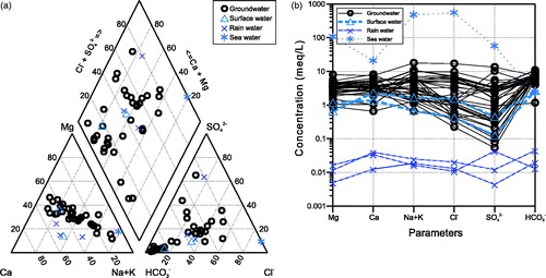
The Piper diagram (Piper, 1944) of Figure 3a indicates a substantial contribution of Mg (up to 50% relative meq/L) and SO₄^2– (up to 65% relative meq/L) in some of the Lake Woods groundwaters. The observed Na–Cl^– to Ca–HCO₃^– transition is typical for rain waters (as the infiltrating starting-point of the groundwaters) evolving progressively from coastal to more inland areas (e.g. Crosbie et al., 2012). The groundwaters are mostly Mg–Ca–HCO₃^– (N = 5), Ca–Mg–HCO₃^– (4), Na–Mg–Ca–HCO₃^––Cl^– (4) or Na–Ca–Mg–HCO₃^––Cl^– (3) type waters, with other water types being represented by only one or two samples. The surface waters are either Ca–Mg–HCO₃^– type water (creek), or Ca–HCO₃^––Cl^– type water (lake). The Schoeller diagram (Schoeller, 1935) of Figure 3b displays the compositional spread of the groundwaters and how they compare with rain water and surface water (as well as with average sea water). It illustrates also how the cation concentrations are less variable than those of Cl^– and especially SO₄^2–. Bicarbonate alkalinity (HCO₃^–), however, has a very restricted concentration range in the Lake Woods ground (and surface) waters. The three average rain-water compositions are relatively similar considering their widely spaced geographic locations (inset, Figure 1).

Figure 3. (a) Piper and (b) Schoeller plots of the Lake Woods water samples. Samples are differentiated by their type: circles, groundwater; triangles, surface (creek or lake) water; crosses, rain water; and star, average sea water (Drever, 1997).

Major ion concentrations in the surface and groundwater samples from Lake Woods are generally consistent with having been derived from the evaporation or evapotranspiration of rain water, using the three aforementioned regional rain-water compositions as proxies for average regional rainfall composition. This means that when plotted against a conservative ion such as Cl^–, those major ions mostly fall within the rain-water evaporation and/or transpiration [hereafter noted as evapo(transpi)ration] trend (RWET) of the regional rain water (Figure 4; Supplementary papers, Figure S3). Some groundwater samples, however, show a slight enrichment in Ca (Supplementary papers, Figure S3a), Mg (Figure 4a) and Na (Supplementary papers, Figure S3b). For K, some samples are enriched, others depleted, relative to the RWET, showing no clear trend with increasing Cl^– (Figure 4b). Most groundwaters are enriched in HCO₃^– (Supplementary papers, Figure S3c) relative to evaporated rain water; conversely, only a few have SO₄^2– concentrations in excess of what would be expected from rain-water evaporation (Figure 4c; see below). Processes that may explain these deviations include mixing and water–mineral interaction (dissolution, precipitation, cation exchange, etc.), as expanded below.

Figure 4. (a) Mg–Cl^–, (b) K–Cl^–, (c) SO₄^2––Cl^–, and (d) Br^––Cl^– scatter plots of the Lake Woods water samples. Samples are differentiated by their type: circles, groundwater; triangles, surface (creek or lake) water; crosses, rain water; and star, average sea water (Drever, 1997). RWET: rain water evapo(transpi)ration trend (shaded field), SWDL: sea water dilution line (solid line).

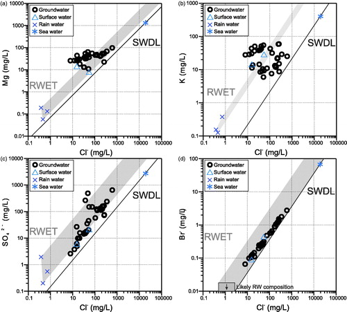
The origin of salinity in groundwater can be inferred from conservative tracers such as Br^– and Cl^–. Sea water has a Cl^–/Br^– (mass) ratio of ∼290 and dilution of sea water (or mixing with fresh meteoric water) will maintain that ratio in the absence of other processes affecting those anions. Initial rain water typically has a Cl^–/Br^– ratio similar to diluted sea water near the coast and an increasingly lower ratio further inland (Herczeg & Edmunds, 2001). At Lake Woods (Figure 4d), the relatively low Cl^–/Br^– ratio of the two surface-water samples (120 and 170) is readily accounted for by the distance from the coast. In the groundwaters, this ratio ranges from 120 to 218. The partly higher Cl^–/Br^– ratio of groundwater, which tends to increase with TDS (r = 0.61, N = 38), is postulated to potentially reflect a minor addition of Cl^– from halite dissolution (halite has a very high Cl^–/Br^– ratio owing to the almost complete exclusion of the Br^– ion from its lattice structure). This is consistent with halite pseudomorphs having been reported in the Namerinni Group and Renner Group basement formations and other evidence of evaporitic minerals and structures in the basement rocks (see stratigraphy information in Supplementary Papers). Alternatively, the minor addition of Cl^– could originate from other minerals (e.g. K-rich muscovite) or fluid inclusions in basement rocks.

Sulfate concentrations relative to Cl^– are almost entirely compatible with those expected from evapo(transpi)ration of the regional rain water (Figure 4b). Perhaps one or two samples with slightly more elevated SO₄^2– concentrations could have experienced an addition of S, which we will revisit when considering the S isotope data (see below).

The minor enrichment in Ca and Mg in some groundwaters (Supplementary papers, Figures S3a and S4a) compared with evaporated rain water noted above is postulated to result from dissolution of carbonate. This carbonate could be a mixture of Ca- and Mg-carbonates, but is more likely to be dolomite ([Ca,Mg]CO₃) owing to (1) a strong correlation observed between dissolved Ca and Mg concentrations (r = 0.83, N = 38), (2) a Ca/Mg (molar) ratio close to unity (as it is in dolomite) in the majority of groundwater samples and (3) the reported occurrence of that mineral in the local aquifers (e.g. Montejinni Limestone; see stratigraphy information in Supplementary Papers). Several groundwater samples, though, have Ca/HCO₃^– (molar) ratios below unity or lower than rain water or surface water (i.e. lower than ∼0.3), especially at low salinities. This implies an additional source of HCO₃^–, which is proposed to result from feldspar dissolution, as developed below.

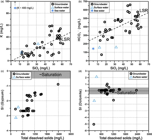
Relative enrichments in Na and K during the evolution of rain water to soil water to groundwater (Supplementary Papers, Figures S3b and 4b), as well as in of HCO₃^– and SiO₂ (Supplementary Papers, Figures S3c, d), are likely due to the incongruent dissolution of feldspar (microcline/orthoclase and the albite-rich end of the plagioclase series), which is consistent with the sandstone/siltstone lithologies of the major regional aquifer (Anthony Lagoon Formation). This reaction is commonly described as the weathering (hydrolysis) of aluminosilicate (e.g. Drever, 1997) following: (Eqn 1) $${2\text{KAlSi}}_3{\mathrm{O}}_8+{2\mathrm{H}}_2{\text{CO}}_3+{9\mathrm{H}}_2\mathrm{O}\rightleftharpoons {\text{Al}}_2{\text{Si}}_2{\mathrm{O}}_5{\left(\text{OH}\right)}_4+{4\mathrm{H}}_4{\text{SiO}}_4+{2\mathrm{K}}^{+}+{2\text{HCO}}_3{}^{-}$$(Eqn 1)

This reaction consumes atmospheric carbon dioxide (as carbonic acid, H₂CO₃), dissolves feldspar (here shown as K-feldspar, KAlSi₃O₈) in the presence of water and results in the common weathering product kaolinite [Al₂Si₂O₅(OH)₄] as well as silicic acid (H₄SiO₄), base cations (K⁺, and/or Na⁺ if present in the initial feldspar) and bicarbonate/alkalinity (HCO₃⁻) in solution. This scenario is consistent with the overall positive correlations observed in sampled groundwater at Lake Woods between SiO₂(aq) and both K (r = 0.68, N = 38; Figure 5a) and HCO₃⁻ (r = 0.62, N = 38; Figure 5b) (SiO₂ concentrations were not reported for the three average rain water samples [Crosbie et al., 2012] and are generally very low in rain water). Note that the highest SiO₂ concentrations in the Lake Woods groundwater are almost exclusively from the southwestern part of the study area (red symbols in Supplementary Papers, Figure S3d), within the Wiso geological region. This is where the more silicic aquifer of the Montejinni Formation (which also contains chert) is expected to exist in subcrop (Verma & Jolly, 1992), with recharge from the lake and via Ashburton Range runoff. Thus, a degree of silicate weathering is inferred to explain the excess cation (K, Ca, Mg, Na), aqueous SiO₂ and bicarbonate concentrations above the RWET trends discussed previously.

Figure 5. (a) K–SiO₂, (b) HCO₃^––SiO₂, (c) gypsum saturation index-total dissolved solids, and (d) dolomite saturation index-total dissolved solids scatter plots of the Lake Woods water samples. Samples are differentiated by their type: circles, groundwater; triangles, surface (creek or lake) water; crosses, rain water; and star, average sea water (Drever, 1997). LSR: least-squares regression line through the groundwater dataset (dashed line). Shaded fields indicate likely saturation with respect to mineral.

The saturation index (SI) of a water sample with respect to a given mineral is defined as: (Eqn 2) $$\text{SI}={\hspace{0.17em}\text{log}\hspace{0.17em}}_{10}\left(\text{IAP}/K_{\text{sp}}\right)$$(Eqn 2) where IAP is the (actual) ion activity product (based on concentrations measured in the sample), and K_sp is the (thermodynamic) solubility product (calculated from thermodynamic data) (Zhu & Anderson, 2002). Figure 5c and d illustrate the SIs of the water samples from the Lake Woods study area with respect to gypsum (CaSO₄•2H₂O) and dolomite. All groundwaters are undersaturated with respect to gypsum (Figure 5c), suggesting that it is unlikely that the waters have been in significant contact with gypsum either in the soils or in the aquifers, given the high solubility of gypsum. As salinity (or total dissolved solids, TDS) increases, there is a tendency for the samples to approach gypsum saturation. In contrast, most samples are in equilibrium with dolomite (–0.5 < SI_dol < +0.5) regardless of salinity; only four or five groundwater samples are either under- or oversaturated with respect to dolomite (Figure 5d). This is consistent with the strong correlation between Ca and Mg noted above suggesting dolomite equilibrium. Other SI calculations (not shown) suggest that most of the sampled waters are close to equilibrium with calcite (CaCO₃; SI_cal mostly from –0.5 to +0.5) and chalcedony (SI_cha from –0.2 to +0.5), reflecting interaction between aquifer carbonate and silicate minerals and groundwaters.

Conversely to the samples most enriched in SiO₂, sourced from the southwest, those containing higher Ca and Mg concentrations tend to originate from the northeastern half of the study area (map not shown). Ca and Mg (molar) concentrations in the groundwaters are strongly correlated (r = 0.83, N = 38) with a slope of 0.70 (Figure 6a). The majority of groundwaters at Lake Woods have Ca/Mg ratios broadly consistent with evapo(transpi)ration of regional rain waters or local surface waters (not shown), with the exception of one sample more enriched in Mg and another more enriched in Ca.

Figure 6. (a) Mg–Ca scatter plot, (b) map of distribution of K/Cl^– (mass) ratio, and (c) K/Cl^– (mass) ratio-total dissolved solids scatter plot of the Lake Woods water samples. Samples are differentiated by their type: circles, groundwater; triangles, surface (creek or lake) water; crosses, rain water; and star, average sea water (Drever, 1997). RWET: rain water evapo(transpi)ration trend (shaded field), SWDL: sea water dilution line (solid line). LSR, least-squares regression line through the groundwater dataset (dashed line).

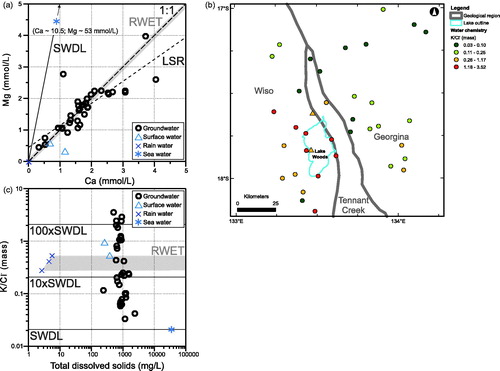
All the water samples collected in this study are enriched in K relative to Cl⁻ compared with sea water, which has a K/Cl⁻ (mass) ratio of ∼0.02 (Figure 6b, c). The groundwaters most enriched in K with 10× or more the sea water ratio (K/Cl⁻ ratios of 0.26 to 3.52, the top two quartiles of the dataset), are all located in the southwestern part of the study area, i.e. over the Wiso and Tennant Creek geological regions (Figure 6b). The three regional rain water samples have K/Cl⁻ ratios of ∼0.28 to 0.54, already more than 10× the sea water ratio (Figure 6c). ‘Excess’ K in rain water in continental settings is well documented and generally attributed to airborne mineral dust from soil (e.g. clay minerals, K salts) as well as emissions from biomass burning (e.g. Honório, Horbe, & Seyler, 2010; Junge & Werby, 1958) being trapped in low clouds and/or rain drops during precipitation events. The two surface waters are slightly more enriched in K than rain water, with K/Cl^– ratios of 0.53 and 0.95. The surface and groundwaters that exhibit K/Cl⁻ ratios more elevated than rain water, in the order of >0.6, must have acquired additional K by interacting with minerals in the soil or aquifers through cation exchange rather than dissolution of K-bearing minerals because their salinity is not markedly greater (in fact arguably slightly lower) than the groundwaters with lower K/Cl^– ratios (see Figure 6c). The regional groundwater dataset also shows K/Cl⁻ ratios exceeding 0.21 (top quartile; ∼10× sea water) and up to 17.5 (nearly 900× sea water) surrounding Lake Woods, although with no obvious relationship to geological regions (Supplementary Papers, Figure S2).

Isotope geochemistry

The stable isotopes of water (δ²H or δ²H_(H2O) and δ¹⁸O_(H2O), reported in ‰ VSMOW) are useful to determine the origin of water and the dominant processes that affect it (e.g. Cook & Herczeg, 2001; Faure & Mensing, 2005). Figure 7a shows the classical δ²H_(H2O)– δ¹⁸O_(H2O) scatter plot of the Lake Woods water samples together with the Global Meteoric Water Line (GMWL: δ²H_(H2O) = 7.96 δ¹⁸O_(H2O) + 8.86; Faure & Mensing, 2005) and the least-squares regression (LSR) line through the Lake Woods groundwater data only (LSR equation: δ²H_(H2O) = 5.24 δ¹⁸O_(H2O) – 17.55; r = 0.97; N = 38). The two outlying surface-water samples with (strongly) positive isotopic values were not included in the LSR to avoid these samples forcing the regression line and to test whether they line up with the trend of the groundwater data. The 38 groundwater samples from the Lake Woods area plot along a line with a slope of 5.24, which is within the range typically interpreted to represent evaporation or evapotranspiration as the samples become progressively enriched in heavy isotopes ²H and ¹⁸O as lighter isotopes preferentially vaporise (Coplen, Herczeg, & Barnes, 2001). Post-monsoon surface (creek) waters plot just to the lower left of the present groundwater data cluster and on the LSR line [13 Newcastle Waters Creek samples collected in March and April 1994 by Yin Foo & Matthews (2000, 2001) have a mean (±SD) δ²H of –70 (±2)‰ and δ¹⁸O of –10 (±0.3)‰). The two surface-water samples collected in this study at the end of the dry season clearly stand out compared with the groundwater samples in this diagram, yet their stable isotopic composition is consistent with a strongly evaporated or evapotranspired local water. One of them (creek water) falls on the regression line for the groundwater; the other (lake water) is slightly above.

Figure 7. (a) δ²H_(H2O)–δ¹⁸O_(H2O) scatter plot of the Lake Woods water samples. Dot-dashed line is the Global Meteoric Water Line (GMWL); dashed line is the least-squares regression (LSR) line through the Lake Woods groundwater data only (see text). (b) δ²H_(H2O)–Cl^– scatter plot of the Lake Woods water samples. (c, d) δ²H_(H2O)–Cl^– scatter plot of the Lake Woods water samples with modelling results overlain for initial δ²H_(H2O) of –65‰ under relative humidity conditions of 0.39 and 0.48 (c), and initial δ²H_(H2O) of –35‰ under relative humidity conditions of 0.45 and 0.58 (d). Samples are differentiated by their type: circles, groundwater; triangles, surface (creek or lake) water; crosses, rain water; and star, average sea water (Drever, 1997).

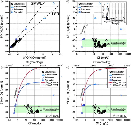
A useful diagram to discriminate between evaporation and evapotranspiration is a plot of δ²H_(H2O) vs a salinity indicator such as Cl^– (Figure 7b). This figure clearly shows all groundwater samples from the Lake Woods study to be dominated by evapotranspiration of water consistent with the three regional rain water compositions. The two surface-water samples, conversely, are strongly affected by purely physical evaporation. These two samples have unusually high positive isotopic values (δ¹⁸O of +10.9 and +16.4‰, and δ²H of +41 and +93‰), which we believe are among the highest O and H isotopic values reported worldwide for surface water, on par perhaps only with those from the Lake Chad region (e.g. Bouchez et al., 2016; Mook, 2001). These extraordinarily elevated isotopic compositions may represent evaporation under very low humidity conditions (I. Cartwright, pers comm; Banks et al., 2009; Cartwright, Hall, Tweed, & Leblanc, 2009; Tweed, Leblanc, Cartwright, Favreau, & Leduc, 2011). We test this hypothesis by modelling the evaporation process as described below.

It is possible to calculate the expected isotopic composition of residual water after evaporation (δ¹⁸O_evap and δ²H_evap) under various relative humidity conditions according to Craig and Gordon (1986) and Gonfiantini (1986). Modelling as detailed in the Supplementary Papers for the known range of initial δ²H (δ²H_i) values of rain water (i.e. from –65 to –35‰) indicates that relative humidity conditions of 0.39 to 0.58 (from 0.39–0.48 for δ²H_i = –65‰ to 0.45–0.58 for δ²H_i = –35‰) are required to produce the isotopic composition of the two surface waters sampled in the Lake Woods study (Figure 7c, d). Using the wet season isotopic data from Yin Foo and Matthews (2000, 2001) as initial conditions (i.e. δ²H_i = –70‰) requires a similarly low relative humidity range (0.38 to 0.47) (plot not shown).

These humidity conditions are entirely compatible with the long term (1976–2005) average meteorological data for the area (BOM, 2016), which is subjected to alternating monsoonal precipitation during summer (November to March) and dry months during winter (May to September), predicating a wide range of annual humidity. If we accept that the surface water’s isotopic composition requires purely physical evaporation under low humidity conditions and that the groundwaters are fully compatible with plant-mediated evapotranspiration of the regional rain water, then we must conclude that there is a disconnect between surface and groundwater in the Lake Woods area, at least as far as stable isotopes δ²H and δ¹⁸O are concerned. This disconnect is likely the result of the sampling campaign having taken place late in the dry season: the surface waters from the creek and the lake are remnants of the last monsoonal rain events and have experienced intense physical evaporation (as opposed to transpiration) since falling as much of the vegetation is dry at this time; the groundwater, conversely, was recharged mainly during the wet season when maximum hydraulic head (surface flooding) promoted infiltration of water into soil and aquifers after having experienced little evaporation (high atmospheric humidity) and significant transpiration by the then luxuriant vegetation.

The S and O isotope values of dissolved SO₄^2– (reported in ‰ VCDT and VSMOW, respectively) were analysed on a subset of 20 Lake Woods groundwater samples. The data form an oblique trend with a positive slope in a δ³⁴S_(SO4)–δ¹⁸O_(SO4) scatter plot (LSR equation: δ³⁴S_(SO4) = 1.99 δ¹⁸O_(SO4) – 5.70; r = 0.71; N = 20) (Figure 8a). The data fall mostly within the ‘Evaporite’ and ‘Atmospheric deposition’ fields at the upper end and the regression line intersects the ‘Soil solution’ end-member field at the lower end (fields from Krouse & Mayer, 2001; Pauwels, Ayraud-Vergnaud, Aquilina, & Molénat, 2010). The data do not appear to trend towards/away from the sea water composition. The observed trend suggests mixing between soil water containing dissolved sulfate with relatively depleted S and O isotopic signatures (near the ‘Soil solution’ field in Figure 8a) with a formation water exhibiting relatively enriched S and O isotope values (near the ‘Evaporite’ field in Figure 8a). One possible source of the ³⁴S-depleted sulfate is through oxidation of reduced biogenic sulfur under saturated conditions (Krouse & Mayer, 2001), where the resulting sulfate can acquire the low δ³⁴S values of biogenic sulfur (down to –30‰) and the low δ¹⁸O values of the ambient groundwater (here –9 to –3‰; see above). Disseminated pyrite, as a possible source of biogenic sulfur, has been reported in lithologies equivalent to the main aquifer in the region (e.g. Kruse & Radke, 2008). The ³⁴S-enriched sulfate, at the other end of the trend, is compatible with the dissolution of evaporite sulfosalt minerals, e.g. gypsum and/or anhydrite. Two possible sources for these minerals exist at Lake Woods, one being recently formed evaporitic minerals in the regolith, the other being syn- or post-depositional evaporites in the basinal formations, which are known to be present in the main aquifers and basement units (e.g. Anthony Lagoon and Gum Ridge formations, Montejinni Limestone; Kruse, Dunster, & Munson, 2013; Verma & Jolly, 1992). To elucidate the relative role of these two sources of sulfate, we need to look at the data from a different angle.

Figure 8. (a) δ³⁴S_(SO4)–δ¹⁸O_(SO4) scatter plot of the Lake Woods water samples, showing the evaporite field from Krouse and Mayer (2001), soil solution field of Pauwels et al. (2010), and the least-squares regression (LSR) line through the Lake Woods groundwater data. (b) δ³⁴S_(SO4)–SO₄^2– scatter plot of the Lake Woods water samples, showing the sea water dilution line (solid line; SWDL), the general trend expected from bacterial sulfate reduction (dashed arrow; BSR); and the general trend exhibited by the Lake Woods water samples (grey arrow). Inset: δ³⁴S_(SO4)–1/SO₄^2– scatter plot, showing the least-squares regression (LSR) line through the Lake Woods groundwater data; and the δ³⁴S_(SO4) end-member composition of sea water (SW; Drever, 1997), regolith gypsum (RG; Chivas et al., 1991; Mernagh et al., 2013; P. de Caritat, unpublished data), and Cambrian marine sulfate (CMS; Claypool et al., 1980; Faure & Mensing, 2005; Krouse, 1980). (c) ⁸⁷Sr/⁸⁶Sr–Sr scatter plot of the Lake Woods water samples, showing the decreasing trend of ⁸⁷Sr/⁸⁶Sr with increasing Sr concentration, the bimodal ⁸⁷Sr/⁸⁶Sr distribution (inset histogram), and spatial distribution of the two populations (inset map). Colours distinguish samples with clustered ⁸⁷Sr/⁸⁶Sr values. (d) ⁸⁷Sr/⁸⁶Sr–δ¹³C_(DIC) scatter plot of the Lake Woods water samples, showing the range of ⁸⁷Sr/⁸⁶Sr (0.710–0.715) with δ¹³C_(DIC) (–12 to –6‰) values of the groundwaters mostly from the less radiogenic population of samples, and spatial distribution (inset map). Arrow indicates the trend associated with carbonate dissolution (e.g. Dogramaci & Herczeg, 2002). Samples are differentiated by their type: circles, groundwater; triangles, surface (creek or lake) water; and star, average sea water (Drever, 1997).

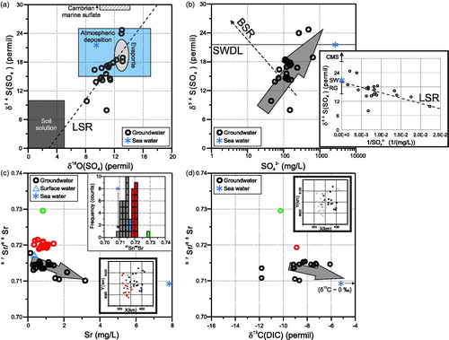
The Lake Woods groundwater data have a positive slope on a δ³⁴S_(SO4)–SO₄^2– scatter plot (LSR equation: SO₄^2– = 21.12 δ³⁴S_(SO4) – 170.84; r = 0.57; N = 20) (Figure 8b), indicating the absence of Bacterial Sulfate Reduction (BSR), which preferentially removes the ³⁴S-depleted SO₄^2– from solution, resulting in a negative slope on such plot (Krouse & Mayer, 2001). Plotting δ³⁴S_(SO4) vs the inverse of SO₄^2– concentration is useful to trace the dominant origin(s) of dissolved S in a hydrological system (Krouse & Mayer, 2001). The bulk of the Lake Woods data (Figure 8b inset) points reasonably strongly towards a single dominant S source with a δ³⁴S_(SO4) value of around +20‰ [LSR equation: δ³⁴S_(SO4) = –451 (1/SO₄^2–) + 20.15; r = 0.59; N = 20]. This can be interpreted as the signature of either sea water (+21‰) in atmospheric deposition, or sulfosalts in the regolith such as gypsum. Regolith gypsum is common in Australia, where it generally has δ³⁴S_(SO4) values ranging from ∼+15‰ to +20‰ depending mainly on distance from the coast (Chivas, Andrew, Lyons, Bird, & Donnelly, 1991; Mernagh et al., 2013; P. de Caritat, unpublished data). It has been shown above, however, that gypsum dissolution is not an important process in the majority of the Lake Woods groundwaters (see Figure 5c). Therefore, the dominant single source of S with a δ³⁴S value of ∼+20‰ is considered to be sea water and is thus inherited from precipitation, specifically during summer monsoons.

Two samples (LW8 and LW9) have been noted to have higher δ³⁴S_(SO4) values (∼+24–25‰) than other Lake Woods groundwater samples, well above the range of sea water and regolith gypsum (Figure 8a, b), which may reflect a contribution of ³⁴S-enriched sulfate from evaporites in the underlying bedrock. These two samples come from adjacent bores in the eastern part of the study area (∼25 km E of Lake Woods) underlain by Georgina Basin sediments, which include the Anthony Lagoon Formation, known to host gypsum/anhydrite (Kruse, 1996; Verma & Jolly, 1992). No published δ³⁴S data on gypsum from the Anthony Lagoon Formation are available, but globally, Cambrian marine gypsum is reported to have δ³⁴S_(SO4) values of around ∼+29 to +33‰ (Claypool, Holser, Kaplan, Sakai, & Zak, 1980; Faure & Mensing, 2005; Krouse, 1980; see hatched field in Figure 8a).

Conversely, the sample (LW13) with the lowest δ³⁴S_(SO4) value (+7.93‰), from a bore located ∼50 km E of Lake Woods, also in the Georgina geological region, may reflect a contribution from a lighter δ³⁴S_(SO4) source. This source could be sulfur from shales, hydrocarbons or coal, or from the oxidation of sulfide minerals (including biogenic pyrite), all of which tend to have an isotopic composition below +5‰ (Caritat, Kirste, Carr, & McCulloch, 2005; Kirste, Caritat, & Dann, 2003; Krouse, 1980). The Georgina Basin is a known conventional and unconventional hydrocarbon province (e.g. Boreham & Ambrose, 2007; Boreham et al., 2013; Draper, 2007) and is likely to host all of the above potential sources of ³⁴S-depleted sulfur.

The Sr isotope systematics indicate a wide spread of relatively elevated ⁸⁷Sr/⁸⁶Sr values for the waters from the Lake Woods study area, ranging mostly from 0.710 to 0.722, with one outlying sample at nearly 0.730 (Figure 8c). Aside from this outlier, the distribution is bimodal (Figure 8c inset histogram), with one sub-population having a mode at ∼0.715, the other at ∼0.721; the two surface-water samples fall between these two populations, at ∼0.717. Three groundwater samples at the lowest end of the range have a Sr isotopic signature close to that of sea water (∼0.709 for modern sea water and ∼0.708–0.7095 for Cambrian sea water; Nicholas, 1996). Spatially, the samples from the less radiogenic sub-population are from the eastern part of the study area corresponding to the Georgina geological region; the samples from the more radiogenic sub-population are from the western part of the study area corresponding to the Wiso geological region; and finally the outlying sample with ⁸⁷Sr/⁸⁶Sr near 0.730 is from the northernmost bore in the northern sliver of the Tennant Creek geological region (see Figure 8c inset map).

There is a notable decrease in ⁸⁷Sr/⁸⁶Sr ratios of the first (Georgina Basin) sub-population of Lake Woods groundwaters as the Sr concentration increases towards a sea-water composition (see Figure 8c) and also perhaps as the δ¹³C_(DIC) increases (Figure 8d). Such trends have been interpreted to reflect the dissolution of marine carbonates (e.g. Dogramaci & Herczeg, 2002), consistent with calcite and dolomite equilibrium as interpreted above. We interpret the second sub-population (Wiso) as representative of interaction with more radiogenic, presumably non-carbonate minerals (e.g. plagioclase, K-feldspar; e.g. McNutt, 2001) in the aquifers of the Wiso Basin. Without further information for isotopic compositions of rocks/minerals in the area, it is unwarranted to speculate further.

In terms of C isotopes, the Lake Woods groundwaters have δ¹³C values between –12 and –6‰ (VPDB), well below the value of sea water (∼0‰; Deuser, Degens, & Guillard, 1968) (Figure 8d); the creek-water sample, however, has a value of –1‰ (not shown). The isotopic values for the groundwaters are consistent with them being in equilibrium (–11 to –8‰; Kendall & Doctor, 2003) with Phanerozoic marine carbonate (δ¹³C ∼0 to +5‰; Ekart, Cerling, Montanez, & Tabor, 1999). This agrees with the groundwaters being at saturation with respect with calcite and dolomite, as discussed above (see Figure 5d). However, we cannot discount that the negative δ¹³C values may also reflect an organic (plant, microbial) influence.

Key implications

Groundwater evolution

Based on the interpretation of chemical and isotopic compositions of the Lake Woods area waters posited above, the factors and processes that control their composition can be described as follows:

1. Moisture with a diluted sea-water geochemical signature forms over the oceans and seaways mostly to the north, northwest and west of the study area. It moves inland and rain falls (during the wet season) over the Lake Woods catchment area and its aquifer recharge zones to its east and southeast, inheriting enhanced major-ion-to-chloride ratios relative to sea water (e.g. K/Cl^–, Ca/Cl^–, SO₄^2–/Cl^–; e.g. see Figure 4; Supplementary Papers, Figure S3). This is the result of both aerosol particle settling during atmospheric transport and the incorporation of terrestrial dust during rain-drop formation and rainfall (in the case of K, biomass burning may also play a role in the region). The two surface-water samples at Lake Woods (i.e. the lake water itself, and the Newcastle Waters Creek feeding it) have a Cl^–/Br^– (mass) ratio of 120 and 170, consistent with that expected from precipitation falling some distance (a minimum of 800–1600 km in the present case) away from the maritime source of moisture (see Davis, Fabryka-Martin, & Wolfsberg, 2004). The groundwaters have a partly overlapping and partly higher Cl^–/Br^– ratio (range 120–218) indicating inheritance of these ions from the local surface (and ultimately rain) water, augmented by a small contribution of Cl^– through minor halite dissolution, as noted in some of the basement units.

2. Evaporation and evapotranspiration of rain water occurs in the catchment area at and immediately below the ground surface. The stable isotope values δ²H and δ¹⁸O of water indicate quite clearly that the two surface-water samples have undergone substantial evaporation under low-moisture conditions, that is, during the dry season (towards the end of which fieldwork occurred). The local surface water starts with a δ²H of –70 (±2)‰ VSMOW and a δ¹⁸O of –10 (±0.3)‰ VSMOW at the end of the wet season (average and standard deviation of 13 post-monsoonal compositions for the Newcastle Waters Creek from Yin Foo & Matthews (2000, 2001)). Ensuing evaporation results in significantly more elevated isotopic values (e.g. δ²H of +41 and +93‰ VSMOW) and Cl^– concentrations (15 and 54 mg/L) relative to regional rain water (δ²H of –70 to –30‰ VSMOW, and Cl^– concentrations of <1 mg/L). In contrast, the groundwater at Lake Woods has a much depleted stable isotopic range, similar to the regional rain water (e.g. δ²H of –70 to –30‰ VSMOW) but with comparable or even more elevated Cl^– concentrations (8–598 mg/L). The latter results indicate that groundwaters have undergone evapotranspiration, not straightforward physical evaporation (see Figure 7b). This interpretation is consistent with isotopic modelling (see Figure 7c, d). Together with the Cl^–/Br^– ratio interpretation, it confirms that under low humidity conditions (dry season), the surface water represents local precipitation that has undergone strong evaporation (particularly elevated δ²H and δ¹⁸O values; moderately high Cl^– concentrations) without significant vegetation-induced transpiration. The groundwater at Lake Woods, in contrast, was recharged during previous wet seasons and was subjected to evapotranspiration (e.g. δ²H similar to precipitation and elevated Cl^–). Overall, our results are consistent with Lake Woods being a losing waterbody, and thus not fed significantly by the underlying aquifer(s).

3. After percolation through soil and recharge into the aquifer, the waters reach equilibrium with dolomite and calcite quite quickly, as indicated by (a) SI_dol close to zero at even low TDS values (see Figure 5d), (b) the strong co-evolution of Ca and Mg, (c) the Ca/Mg (mol) ratio close to unity for most groundwater samples (see Figure 6a), and (d) the δ¹³C values (–12 and –6‰ VPDB) consistent with marine carbonate dissolution from aquifer formations being the source of the DIC.

4. Dissolution of either regolith or evaporitic gypsum occurs to only a very minor extent in the system, as SI_gyp indicates undersaturation at all salinities with a slow evolution towards equilibrium (see Figure 5c). Two samples have elevated δ³⁴S_(SO4) values (∼+24‰ VCDT), which may indicate dissolution of Cambrian marine sulfate (see Figure 8a), present in the aquifer formations.

5. BSR is not occurring in this groundwater system.

6. Hydrolysis of K-feldspar (and plagioclase) takes place during transit of the groundwater in the aquifers, as shown by the strong correlation of the reaction by-products silicic acid (H₄SiO₄ measured as SiO₂), base cations (K and/or Na, Ca; see Figure 5a), and alkalinity (HCO₃⁻; see Figure 5b). This is consistent with the Sr isotope results (see below).

7. Minor halite dissolution occurs where groundwater comes into contact with basement units, e.g. the Renner Group, as indicated by the Cl^–/Br^– ratio, discussed above.

8. Strontium isotope ratios of the groundwaters reflect the geological regions they occur in: samples collected from bores in the Wiso geological region west of the Ashburton Range have more radiogenic ⁸⁷Sr/⁸⁶Sr ratios consistent with the partly siliciclastic (sandstone, mudstone) nature of the Montejinni and Point Wakefield aquifers there. On the east side of the range, less radiogenic ⁸⁷Sr/⁸⁶Sr ratios reflect the dominantly carbonate nature of the Anthony Lagoon and Gum Ridge aquifers.

The results of the present study suggest that Lake Woods is not a hydrologically closed system. Lake water recharge is predominantly by surface-water flow from Newcastle Waters Creek following periodic monsoonal rainfall, with subordinate replenishment of lake waters via runoff from numerous small creeks draining the rocky slopes of the Ashburton Range. In turn, Lake Woods recharges underlying aquifers, particularly the porous Cambrian Montejinni Limestone of the Wiso Basin (Verma & Jolly, 1992). This process impedes the accumulation and retention of salts in the lakebed despite high rates of solar radiation that would otherwise tend to promote formation of evaporite minerals. Only ephemeral efflorescent salts are expected to precipitate at the lake margins under such prevailing conditions.

Lake Woods has a history of cyclic hydrological changes dating back to the early Pleistocene that is preserved in a complex series of outer shorelines and sand ridges. Application of multiple luminescence dating techniques has identified four major depositional events (Bowler et al., 1998). Lake Woods lacks the surface retention of salts typical of other lakes in central Australia. Although episodic drying of the relatively large lake through recent millennia may have resulted in concentrations of dissolved salts, these have not been retained in the surficial landscape. There may have been extended periods in the geological past, for example during the hyperarid Last Glacial Maximum (LGM) around 20 ka, when salts accumulated in the lakebed. During the LGM, vegetation decreased across Australia because of extreme aridity, and water-tables rose (owing to the combined reduction in vegetation, temperature and evapotranspiration), to discharge into lakebeds (Bowler et al., 1998). Lake settings became ‘groundwater windows’ from which salts precipitated in response to evaporative concentration. During periods of extreme aridity across the continent, salts were remobilised from salt lakes by enhanced eolian activity and deposited further afield. It is assumed that any such salts in Lake Woods, had they accumulated in the past, would have long since been flushed into underlying aquifers and down the northwestward-groundwater gradient to the Daly Basin once climatic conditions ameliorated. Moreover, any windborne salts sourced from lakes in the central Australian region, along with salts arriving in monsoonal rainfall, may have readily been sequestered into smectite clays of surrounding black soil plains, to contribute solutes to the groundwater system.

Mineral prospectivity

Mineral prospectivity of the Lake Woods region is investigated within the mineral system framework (Knox-Robinson & Wyborn, 1997; Murphy et al., 2011; Wyborn, Heinrich, & Jaques, 1994). Although there is significant enrichment of K in the input fluids to the Lake Woods catchment compared with Cl^– content, its total concentration remains lower than or equal to that in sea water (i.e. ∼399 mg/L). The fact that solute-laden groundwater does not discharge at Lake Woods, but rather seasonal lake water percolates downward into underlying aquifers, implies that solutes are transported into the aquifers rather than retained in the lake system, yielding unfavourable conditions for precipitation and preservation of salts in the surficial environment.

In order to form economic concentrations of potash it would be necessary to pump the groundwater into solar evaporation ponds where it could undergo intense evaporitic concentration. The most concentrated groundwaters in this region contain up to ∼50 mg/L K. This means that it would be necessary to evaporate 10.5 m³ of water to extract one kg of KCl (assuming 100% recovery). The economics of such a process would depend on the time taken to evaporate the water, the purity of the product, infrastructure costs and market imperatives. Furthermore, the cutoff grade for extraction of K brines is variable, and historically, development has not been based on true economic merit (Garrett, 1996). Current commercial K brines range in concentration from 1500 to 40 000 mg/L (Garrett, 1996; Kilic & Kilic, 2010).

Several ephemeral lakes on the Barkly Tableland east of Lake Woods, including Tarrabool Lake and Lake Sylvester, are surrounded by bedrock units that contain evaporites and local groundwaters are enriched in K compared with sea water, with K/Cl^– >10× sea water (Jaireth et al., 2012). Whether these numerous lakes function as discharge lakes (i.e. in receipt of groundwater), or as recharge lakes (i.e. episodic lake waters being flushed to the underlying aquifer), analogous to Lake Woods, has not been established. Given the widespread occurrence of groundwaters containing high K concentrations in the plains east of Lake Woods and a lack of information about connectivity between surface water and groundwater at Lake Sylvester, Tarrabool Lake and neighbouring satellite lakes, this region warrants investigation before prospectivity for commodity salts can be disregarded.

The Li/Cl^– ratio of the Lake Woods groundwaters ranges from 0.4 to ∼400 times its value in sea water (8.8 × 10⁻⁶). Lithium mineralised regions around the world mostly have waters with Li/Cl^– ratios of 50 to >500 times the sea-water value, and Lake Frome, which has been touted as a potential Li target in Australia (ASX, 2011), has Li/Cl^– values mostly <50 times sea water (Mernagh et al., 2013). Current or recently producing Li-bearing salt lakes contain brines with Li concentrations ranging from 50 to 1400 mg/L, although the lowest productive grade for assessing prospectivity is currently 200 mg/L Li (Gruber et al., 2011). In that regard, Li concentrations in Lake Woods groundwater are negligible (<0.2 mg/L).

The B/Cl^– (mass) ratio of the Lake Woods groundwaters ranges from 2 to 284 times its value in sea water (2.3 × 10⁻⁴). Boron mineralised regions around the world mostly have waters with B/Cl^– ratios of 10 to >50 times the sea-water value (Mernagh et al., 2013).

These results suggest that the Lake Woods groundwaters, considered in isolation, potentially have a suitable composition for a B and/or Li mineral potential to be present. As discussed before, however, the hydrological conditions (discharging lake) are not favourable to the development of an economic resource.

Finally, the mineral potential of the Lake Woods region for uranium (U) deposits has not been previously assessed in detail. The groundwaters show signs of moderate U enrichment (U up to 13 µg/L, which is below the Australian Drinking Water Guidelines [ADWG, 2018] value of 17 µg/L), although the U/Cl^– ratio can be up to 7000 times its value in sea water. The surface regolith and rocks in the Lake Woods study area have low to moderate U content (mostly <1.5 ppm U) as shown by airborne radiometric data (Minty, Franklin, Milligan, Richardson, & Wilford, 2009), or by more direct National Geochemical Survey of Australia measurements (mostly <2 mg/kg total U in coarse surface sediments, and mostly <0.6 mg/kg Aqua Regia digestible U in coarse surface sediments; Caritat & Cooper, 2011; Reimann & Caritat, 2017). The compilation of Mernagh et al. (2013) did not highlight the Lake Woods region as having a particularly high U mineral potential.

Conclusions

The hydrogeochemical analysis developed here has identified the major chemical processes controlling groundwater composition in the Lake Woods area, including evapotranspiration and water–mineral interaction (i.e. dissolution of carbonates, silicate hydrolysis and to a lesser extent dissolution of evaporite minerals such as halite, gypsum and/or anhydrite). However, the surface (lake and creek) waters collected during the dry season have exceptionally enriched O and H isotope values (δ¹⁸O of +10.9 to +16.4‰ VSMOW and δ²H of +41 to +93‰ VSMOW), which we contend resulted from evaporation (and not evapotranspiration) during low humidity conditions (dry season).

The mineral systems analysis provided here has identified several factors favourable for productive potash systems. For example, the Georgina Basin contains evaporite-bearing bedrock units and extensive aquifers for which geochemical analysis of the groundwaters indicates source fluids enriched in K. However, some critical factors of the mineral system are not present in ephemeral lake systems of the region. The Lake Woods system, for example, is not hydrologically closed and is not a lake that is dominated by groundwater processes. Consequently, it lacks a suitable intrinsic enrichment mechanism (e.g. continuous intense evaporation) to generate high concentrations of target elements in the fluids within the near-surface environment. On the other hand, numerous other ephemeral lakes in the Georgina Basin east of Lake Woods, where groundwaters are similarly enriched in K, have not been investigated to date. These areas, including Lake Sylvester and Tarrabool Lake, may be more prospective than Lake Woods if groundwaters are discharging in these ephemeral lakebeds and salt precipitation is occurring, and an all-inclusive mineral system is operating. The Li, B and U resource potential of Lake Woods appears limited based on the hydrological and surface geology conditions, even though at first glance the groundwaters may be anomalous in these elements. The present study has, accordingly, highlighted the importance of accounting for all the critical factors of a mineral system in assessing a region’s prospectivity for economic mineral deposits.

Acknowledgements

We thank the landowners for granting access to their land and water bores. The satellite image used in Figures 1a and S1b was provided through Esri (2016) based on data from Esri, DigitalGlobe, GeoEye, Earthstar Geographics, CNES/Airbus DS, USDA, USGS, AEX, Getmapping, Aerogrid, IGN, IGP, swisstopo and the GIS User Community. Regional hydrogeological information and dissolved K data were provided by Steven Tickell, NT Department of Environment and Natural Resources. Internal (Geoscience Australia) reviews by Andrew Feitz and Luke Wallace contributed to improving the final manuscript and are much appreciated. Journal referees are warmly thanked for providing detailed and constructive critiques of our original manuscript. Published with permission from the Chief Executive Officer, Geoscience Australia.

References

- ADWG (Australian Drinking Water Guidelines). (2018). National water quality management strategy – Australian Drinking Water Guidelines 6, 2011 (version 3.5 Updated August 2018). Canberra ACT: National Health and Medical Research Council, Natural Resources Management Ministerial Council.
- ASUD (Australian Stratigraphic Units Database). (2016). Australian stratigraphic units database [Dataset]. Canberra ACT: Geoscience Australia. Retrieved from http://www.ga.gov.au/data-pubs/data-standards/reference-databases/stratigraphic-units
- ASX (Australian Securities Exchange). (2011). ERO to commence major 2011 drilling program. Retrieved from http://www.tycheanresources.com/investors/asx/2011/ero_asx20110124.pdf
- Banks, E. W., Simmons, C. T., Jolly, I. D., Doble, R. C., McEwan, K. L., & Herczeg, A. L. (2009). Interactions between a saline lagoon and a semi-confined aquifer on a salinized floodplain of the lower River Murray, southeastern Australia. Hydrological Processes, 23, 3415–3427.
- Blake, D., & Kilgour, B. (1998). Geological Regions of Australia 1:5 000 000 scale [Dataset]. Canberra ACT: Geoscience Australia. Retrieved from http://www.ga.gov.au/metadata-gateway/metadata/record/gcat_a05f7892-b237-7506-e044-00144fdd4fa6/Geological+Regions+of+ Australia%2C+1%3A5+000+000+scale
- BOM (Bureau of Meteorology (2016). ) Maps of average conditions. Canberra ACT: Bureau of Meteorology. Retrieved from http://www.bom.gov.au/climate/averages/maps.shtml
- BOM (Bureau of Meteorology) (2017). Wind speed and direction rose (Tindal). Canberra ACT: Bureau of Meteorology. Retrieved from http://www.bom.gov.au/cgi-bin/climate/cgi_bin_scripts/windrose_selector.cgi?period=OcttoApr&type=9&location=14932&Submit=Get+Rose
- Boreham, C. J., & Ambrose, G. J. (2007). Cambrian petroleum systems in the southern Georgina Basin, Northern Territory, Australia. In T. J. Munson & G. J. Ambrose (Eds.), Proceedings of the Central Australian Basins Symposium, Alice Springs, 16–18th August, 2005 (pp. 254–281). Darwin, NT: Northern Territory Geological Survey, Special Publication.
- Boreham, C. J., Edwards, D. S., Hall, L., Bernecker, T., Carr, L. K., Chen, J., … Horsfield, B. (2013). Unconventional Middle Cambrian petroleum systems in the Georgina Basin, Australia. Paper presented at The American Association of Petroleum Geologists, Hedberg Conference, Beijing, China, 21–24 April 2013. Tulsa, OK: AAPG.
- Bouchez, C., Goncalves, J., Deschamps, P., Vallet-Coulomb, C., Hamelin, B., Doumnang, J.-C., & Sylvestre, F. (2016). Hydrological, chemical, and isotopic budgets of Lake Chad: A quantitative assessment of evaporation, transpiration and infiltration fluxes. Hydrology and Earth System Sciences, 20, 1599–1619.
- Bowler, J. M., & Teller, J. T. (1986). Quaternary evaporites and hydrological changes, Lake Tyrrell, north-west Victoria. Australian Journal of Earth Sciences, 33, 43–63.
- Bowler, J. M., Duller, G. A. T., Perret, N., Prescott, J. R., & Wyrwoll, K.-H. (1998). Hydrological changes in monsoonal climates of the last glacial cycle: Stratigraphy and luminescence dating of Lake Woods, N.T., Australia. Palaeoclimates: Data and Modelling, 3, 179–207.
- Cartwright, I., Hall, S., Tweed, S., & Leblanc, M. (2009). Geochemical and isotopic constraints on the interaction between saline lakes and groundwater in southeast Australia. Hydrogeology Journal, 17, 1991–2004.
- Chivas, A. R., Andrew, A. S., Lyons, W. B., Bird, M. I., & Donnelly, T. H. (1991). Isotopic constraints on the origin of salts in Australian playas. 1. Sulphur. Palaeogeography, Palaeoclimatology, Palaeoecology, 84, 309–332.
- Claypool, G. E., Holser, W. T., Kaplan, I. R., Sakai, H., & Zak, I. (1980). The age curves of sulfur and oxygen isotopes in marine sulfate and their mutual interpretation. Chemical Geology, 28, 190–260.
- Cook, P. G., & Herczeg, A. L. (Eds.) (2001). Environmental tracers in subsurface hydrology (second printing). Boston, MA: Kluwer Academic Publishers.
- Coplen, T. B., Herczeg, A. L., & Barnes, C. (2001). Isotope engineering—Using stable isotopes of the water molecule to solve practical problems. In P. G. Cook & A. L., Herczeg (Eds.), Environmental Tracers in Subsurface Hydrology (Second Printing) (pp. 79–110). Boston, MA: Kluwer Academic Publishers.
- Craig, H., & Gordon, L. I. (1986). Deuterium and oxygen-18 variations in the ocean and atmosphere. In E. Tongiorgi (Ed.), Stable Isotopes in Oceanographic Studies and Palaeotemperatures (pp. 9–130). Pisa, Italy: Consiglio Nazionale Delle Ricerche Laboratorio di Geologia Nucleare.
- Crosbie, R., Morrow, D., Cresswell, R., Leaney, F., Lamontagne, S., & Lefournour, M. (2012). New insights to the chemical and isotopic composition of rainfall across Australia. Canberra, ACT: CSIRO Water for a Healthy Country Flagship, Australia.
- Davis, S. N., Fabryka-Martin, J. T., & Wolfsberg, L. E. (2004). Variations of bromide in potable ground water in the United States. Ground Water, 42, 902–909.
- de Caritat, P., Kirste, D., Carr, G., & McCulloch, M. (2005). Groundwater in the Broken Hill region, Australia: Recognising interaction with bedrock and mineralisation using S, Sr and Pb isotopes. Applied Geochemistry, 20, 767–787.
- de Caritat, P., & Cooper, M. (2011). National geochemical survey of Australia: The geochemical atlas of Australia (Record 2011/20, 2 Volumes, 557 p). Canberra ACT: Geoscience Australia.
- DIIS (Department of Industry, Innovation and Science) (2016). Exploring for the future. Canberra ACT: Department of Industry, Innovation and Science. Retrieved from http://industry.gov.au/resource/Programs/Pages/Exlporing-for-the-Future.aspx
- Deuser, W. G., Degens, E. T., & Guillard, R. R. L. (1968). Carbon isotope relationships between plankton and sea water. Geochimica et Cosmochimica Acta, 32, 657–660.
- Dogramaci, S. S., & Herczeg, A. L. (2002). Strontium and carbon isotope constraints on carbonate-solution interactions and inter-aquifer mixing in groundwaters of the semi-arid Murray Basin, Australia. Journal of Hydrology, 262, 50–67.
- Draper, J. (2007). Georgina Basin – an early Palaeozoic carbonate petroleum system in Queensland. Australian Petroleum Production and Exploration Association Journal, 47, 105–124.
- Drever, J. I. (1997). The geochemistry of natural waters: Surface and groundwater environments (3rd ed.). New Jersey, NJ: Prentice Hall.
- Ekart, D. D., Cerling, T. E., Montanez, I. P., & Tabor, N. J. (1999). A 400 million year carbon isotope record of pedogenic carbonate: implications for paleoatmospheric carbon dioxide. American Journal of Science, 299, 805–827.
- Esri (Environmental Systems Research Institute). (2016). ArcGIS world imagery. Redlands CA: Environmental Systems Research Institute. Retrieved from: http://goto.arcgisonline.com/maps/World_Imagery
- Faure, G., & Mensing, T. M. (2005). Isotopes—Principles and applications. Hoboken, NY: John Wiley & Sons.
- Garrett, D. E. (1996). Potash—Deposits, processing, properties and uses. New York NY: Chapman and Hall.
- Gonfiantini, R. (1986). Environmental isotopes in lake studies. In P. Fritz & J. C., Fontes (Eds.), Handbook of environmental isotope geochemistry. The terrestrial environment (Vol. 2, pp. 113–186). Amsterdam: Elsevier.
- Gruber, P. W., Medina, P. A., Keoleian, G. A., Kesler, S. E., Everson, M. P., & Wallington, T. J. (2011). Global lithium availability: A constraint for electric vehicles? Journal of Industrial Ecology, 15, 760–775.
- Herczeg, A. L., & Edmunds, W. M. (2001). Inorganic ions as tracers. In P. G. Cook & A. L. Herczeg (Eds.), Environmental tracers in subsurface hydrology (Second Printing) (pp. 31–77). Boston, MA: Kluwer Academic Publishers.
- Honório, B. A. D., Horbe, A. M. C., & Seyler, P. (2010). Chemical composition of rainwater in western Amazonia – Brazil. Atmospheric Research, 98, 416–425.
- Jaireth, S., Bastrakov, E., Wilford, J., English, P., Magee, J., Clarke, J., … Thomas, M. (2012). Salt lakes prospective for potash deposits (First edition). 1:5 000 000 scale. Canberra ACT: Geoscience Australia, Geocat No. 75875. Retrieved from https://d28rz98at9flks.cloudfront.net/76454/MAP_3_Potash_36x54_600dpi.pdf
- Jasinski, S. M. (2015). Potash. Reston VA: USGS 2013 Minerals Yearbook, 58.1–58.6. Retrieved from http://minerals.usgs.gov/minerals/pubs/commodity/potash/myb1-2013-potas.pdf
- Junge, C. E., & Werby, R. T. (1958). The concentration of chloride, sodium, potassium, calcium, and sulfate in rain water over the United States. Journal of Meteorology, 15, 417–425.
- Kendall, C., & Doctor, D. H. (2003). Stable isotope applications in hydrologic studies. In J. I. Drever (Ed.), Surface and ground water, weathering, and soils. Treatise on GEochemistry, 5 (pp. 319–364). Amsterdam: Elsevier.
- Kilic, O., & Kilic, A. M. (2010). Salt crust mineralogy and geochemical evolution of the Salt Lake (Tuz Gölü), Turkey. Scientific Research and Essays, 5, 1317–1324.
- Kirste, D., Caritat, P. de, & Dann, R. (2003). The application of the stable isotopes of sulfur and oxygen in groundwater sulfate to mineral exploration in the Broken Hill region of Australia. Journal of Geochemical Exploration, 78-79, 81–84.
- Knapton, A. (2006). Regional groundwater modelling of the Cambrian Limestone Aquifer System of the Wiso Basin, Georgina Basin and Daly Basin. A report prepared by NRETA Land and Water Division (Technical Report No. 29/2006A). Darwin, NT: NT Department of Natural Resources, Environment & The Arts.
- Knox-Robinson, C. M., & Wyborn, L. A. I. (1997). Towards a holistic exploration strategy: Using geographic information systems as a tool to enhance exploration. Australian Journal of Earth Sciences, 44, 453–463.
- Krouse, H. R. (1980). Sulphur isotopes in our environment. In P. Fritz & J.-C. Fontes (Eds.), Handbook of environmental isotope geochemistry (pp. 435–471). Amsterdam: Elsevier.
- Krouse, H. R., & Mayer, B. (2001). Sulphur and oxygen isotopes in sulphate. In P. G. Cook & A. L. Herczeg (Eds.), Environmental tracers in subsurface hydrology (Second Printing) (pp. 195–231). Boston, MA: Kluwer Academic Publishers.
- Kruse, P. D. (1996). Helen Springs Stratigraphic Drilling 1996 – NTGS96/1 Nilly Waterhole (Technical Report, GS96/004). Darwin, NT: NT Department of Mines and Energy.
- Kruse, P. D., & Radke, B. M. (2008). Ranken-Avon Downs, Northern Territory. 1:250 000 geological map series explanatory notes, SE 53-16, SF 53-04. Darwin, NT: Northern Territory Geological Survey.
- Kruse, P. D., Dunster, J. N., & Munson, T. J. (2013). Chapter 28 Georgina basin. In M. Ahmad & T. J. Munson (compilers), Geology and mineral resources of the northern territory (pp. 28:1–28:56). Darwin, NT: Northern Territory Geological Survey, Special Publication 5.
- Magee, J. W., & Miller, G. H. (1998). Lake Eyre palaeohydrology from 60 ka to the present: beach ridges and glacial maximum aridity. Palaeogeography, Palaeoclimatology, Palaeoecology, 144, 307–329.
- McNutt, R. H. (2001). Strontium isotopes. In P. G. Cook & A. L. Herczeg (Eds.), Environmental tracers in subsurface hydrology (Second Printing) (pp. 233–260). Boston, MA: Kluwer Academic Publishers.
- Mernagh, T. P., Bastrakov, E. N., Clarke, J. D. A., Caritat, P. de, English, P. M., Howard, F. J. F., … Wilford, J. R. (2013). A review of Australian salt lakes and assessment of their potential for strategic resources. Canberra ACT: Geoscience Australia Record, 2013/39, 243 p. Retrieved from https://d28rz98at9flks.cloudfront.net/76454/Rec2013_039.pdf
- Mernagh, T. P., Bastrakov, E. N., Jaireth, S., Caritat, P. de, English, P. M., & Clarke, J. D. A. (2016). A review of Australian salt lakes and associated mineral systems. Australian Journal of Earth Sciences, 63, 131–157.
- Minty, B., Franklin, R., Milligan, P., Richardson, M., & Wilford, J. (2009). The radiometric map of Australia. Exploration Geophysics, 40, 325–333.
- Mook, W. M. E. (2001). Environmental isotopes in the hydrological cycle. Principles and applications. UNESCO/IAEA Series, 39. Vienna: IAEA. Retrieved from http://www-naweb.iaea.org/napc/ih/IHS_resources_publication_hydroCycle_en.html
- Murphy, F. C., Hutton, L. J., Walshe, J. L., Cleverley, J. S., Kendrick, M. A., McLellan, J., … Nortje, G. S. (2011). Mineral system analysis of the Mt Isa–McArthur River region, Northern Australia. Australian Journal of Earth Sciences, 58, 849–873.
- Nicholas, C. J. (1996). The Sr isotopic evolution of the oceans during the 'Cambrian Explosion'. Journal of the Geological Society, 153, 243–254.
- Pauwels, H., Ayraud-Vergnaud, V., Aquilina, L., & Molénat, J. (2010). The fate of nitrogen and sulfur in hard-rock aquifers as shown by sulfate-isotope tracing. Applied Geochemistry, 25, 105–115.
- Piper, A. M. (1944). A graphical procedure in the geochemical interpretation of water analyses. Transactions, American Geophysical Union, 25, 914–923.
- Raymond, O. L., Liu, S., Gallagher, R., Zhang, W., & Highet, L. M. (2012). Surface geology of Australia, 1:1 million scale dataset 2012 edition [Dataset]. Canberra ACT: Geoscience Australia. Retrieved from http://www.ga.gov.au/metadata-gateway/metadata/record/74619/
- Reimann, C., & Caritat, P. de (2017). Establishing geochemical background variation and threshold values for 59 elements in Australian surface soil. The Science of the Total Environment, 578, 633–648.
- Schoeller, H. (1935). Utilité de la notion des échanges de bases pour la comparison des eaux souterraines. Société Géologique France Bulletin (Série S), 5, 651–657.
- Stewart, A. J., Raymond, O. L., Totterdell, J. M., Zhang, W., & Gallagher, R. (2013). Australian geological provinces, 2013.01 edition [Dataset]. Canberra ACT: Geoscience Australia. Retrieved from http://www.ga.gov.au/metadata-gateway/metadata/record/gcat_c3fac1d5-48c1-624e- e044-00144fdd4fa6/Australian+Geological+Provinces%2C+2013.01+ edition
- Tickell, S. J. (2003). Water resource mapping: Barkly tablelands. Darwin NT: Northern Territory Department of Infrastructure, Planning and Environment.
- Tweed, S., Leblanc, M., Cartwright, I., Favreau, G., & Leduc, C. (2011). Arid zone groundwater recharge and salinisation processes: an example from the Lake Eyre Basin, Australia. Journal of Hydrology, 408, 257–275.
- Verma, M. N., & Jolly, P. B. (1992). Hydrogeology of Helen Springs. Explanatory notes for 1:250 000 Scale Map (Northern Territory Power and Water Authority Report 50/1992). Darwin, NT: Northern Territory Power and Water Authority.
- Winter, T. C., Harvey, J. W., Franke, O. L., & Alley, W. M. (1998). Groundwater and surface water: A single resource. U.S. Geological Survey Circular 1139. Denver, CO: U.S. Government Printing Office.
- Wyborn, L. A. I., Heinrich, C. A., & Jaques, A. L. (1994). Australian Proterozoic mineral systems: Essential ingredients and mappable criteria. In The Australian Institute of Mining and Metallurgy (AusIMM) Annual Conference, Darwin, 5–9 August 1994 (pp. 109–115). Melbourne, VIC: AusIMM.
- Yin Foo, D., & Matthews, I. (2000). Water resources assessment of the Sturt Plateau technical data report (Report 31/2000D). Darwin, NT: Natural Resources Division, Department of Lands Planning and Environment.
- Yin Foo, D., & Matthews, I. (2001). Hydrogeology of the Sturt Plateau 1:250 000 scale map explanatory notes (Report 17/2000D). Darwin, NT: Department of Infrastructure, Planning and Environment.
- Zhu, C., & Anderson, G. (2002). Environmental applications of geochemical modelling. Cambridge, UK: Cambridge University Press.