Towards quantifying uncertainties in geological models for mineral resource estimation through outside-in deposit-scale structural geological analysis

Abstract

Mineral Resource downgrades can be prevented by integrating better structural geological interpretations into project evaluations. Geological modelling for Mineral Resource estimation is presented as a systematic process of structural geological analysis at the deposit-scale using drill-sampled grade data. The initial step in this process is to use Maximum Intensity Projection (MIP) rendering to interpret axial symmetry and its orientation from the grade interval mid-points at the deposit-scale, thus reducing the modelling process’s degrees of freedom to only three—estimating the prolateness of the grade or lithological distribution. This approach contrasts with the brute-force methods for assessing modelling uncertainty because the axial direction is fixed to the down-plunge orientation, thus eliminating from the outset, structurally implausible geometric configurations and unrealistic geological scenarios common in brute-force methods. Adopting this new approach of creating geological models means moving away from conventional mining industry methods that prioritise operational considerations in constructing resource estimates but fail to explain the geometric complexities of mineral deposits. We use experiments and a practical case study of a historical gold mine in Western Australia to highlight the significance of analysing the structural control of a gold deposit at the deposit-scale using raw grade data. Our research is based on anecdotal evidence suggesting that erroneous geological modelling leads to unforeseen Mineral Resource downgrades. However, we cannot confirm this hypothesis because there have been few, if any, independent public inquiries into Mineral Resource downgrades. To establish the underlying reasons for significant resource downgrades with certainty, impartial investigations (modelled on accident investigations in the aviation industry) are imperative.

KEY POINTS

1. There is a general lack of incorporating structural geological knowledge in creating resource models, which can lead to poor outcomes such as Mineral Resource downgrades.

2. Structural geological analysis of drill-sampled raw grade data allows the structural controls on a deposit to be better understood.

3. We offer a simple workflow for understanding and modelling these patterns.

Keywords:

• Maximum Intensity Projection
• structural geology
• resource geology
• gold
• implicit modelling
• axial symmetry
• resource risk
• mineral resources

Introduction

The paper introduces a practical structural geological technique not currently used by practitioners in resource estimation that has the potential to significantly improve the accuracy of their estimates. We present some steps towards quantifying the uncertainties of geological models.

In recent years, multiple instances of Mineral Resource¹ downgrades have negatively affected investor confidence. In publicly disclosed technical reports, such as those reported in compliance with the Canadian National Instrument (NI) 43-101 (Canadian Institute of Mining, 2022; CSA, 2011; Pressacco et al., 2019), the role of structural geological input, or even geological input in general, is rarely acknowledged in the resource estimation process for mineral deposits. In fact, structural geological input is typically not included in the resource estimation process, irrespective of the deposit’s subsequent economic success or failure. The lack of structural input is a result of the historical development of geostatistical estimation methods and geological modelling, which were primarily influenced by surveying rather than the geological discipline (Krige, 1951; Matheron, 1963). Mineral deposits are largely controlled by geological variabilities commonly governed by structural geological controls. Therefore, incorporating a comprehension of structural geology into resource estimations is a logical approach that can enhance their accuracy.

Interpreting the structural configuration of any deposit as input into the resource estimation process is often an intimidating hurdle for most geologists, especially if the modeller has little or no understanding of structural geological principles. In addition, most deposits lack structural geological data, thus making it impossible to incorporate structural information into the resource estimation process.

The methodology discussed in this paper does not require traditional structural geological data collected from the field. Instead, it uses the readily available grade data obtained through drilling—data that are also the primary focus of resource estimators. Using the scientific principle of fundamental structural geometry, we develop a straightforward deposit-scale structural model using grade data. This model helps create geological and resource models and helps identify additional targets for further exploration. This paper also explores the problems that can arise in resource modelling when geological factors, particularly structural geological controls, are not sufficiently considered.

Structural geology and its connection to resource estimations

A comprehensive three-dimensional (3D) geology model is essential for accurately estimating the resources of a deposit and is the foundation for the entire resource estimation process, ensuring accuracy and reliability of the final results. This model should represent the deposit’s geology as understood at the time of estimation, and it should include structural geometry, lithology, alteration, and all other relevant data (Vann & Stewart, 2011). All subsequent steps, such as resource domaining, variography and estimation parameters, should incorporate the knowledge gained from this detailed 3D geology model.

Textbooks on resource geology generally emphasise the fundamental importance of geology (Abzalov, 2016; Coombes, 2008). Although these works provide an excellent overview of resource estimation practices, they commonly assume the existence of an accurate underlying geology model. Sterk et al. (2019) address the lack of textbook guidance for constructing geological or structural models for resource estimation. Introductory training courses in resource geology may touch on the importance of geology in model construction, but tend to place more emphasis on software-based workflows or statistical analyses that are performed on already modelled domains (McManus et al., 2021; Sterk et al., 2019). These courses generally assume that trainees already have the modelling skills to create these volume domains and seldom provide detailed explanations on how to construct the underlying 3D geological volumetric models necessary for resource estimation. If the trainees do have these skills, it is also assumed that they can recognise the potential geological variations that may occur in a given scenario, which involves the necessary step of excluding domain geometry variations that are geologically implausible. In contrast to a geostatistician, who may have limited knowledge of geology and assume that many geometric variations are probable, there are geological and structural constraints that make some geological models highly improbable. The relationship between structural geology, geological modelling and resource estimation is rarely addressed in the literature (Cowan, 2014; Stoch et al., 2022), and this relationship is the primary focus of this paper.

Where structural geological controls of a deposit are not properly understood, the resulting Mineral Resource model will likely be fundamentally flawed. An independent investigation or resource audit typically verifies the statistical validity of a Mineral Resource, but not the geological soundness of the model. An audit of the geological soundness is crucial to test the model sufficiently and to identify and challenge errors and assumptions that may have been introduced through ‘groupthink’ (Phillips, 2011). The primary issue is that while geostatistical methods can be used to model and evaluate intra-model variations, there is currently no equivalent methodology for analysing inter-model variations, particularly in terms of ruling out implausible geological models. The persistence of surprise Mineral Resource downgrades in 2023, two decades after the advent of rapid implicit geological modelling (Cowan et al., 2002, 2003), could be partly attributed to failing to recognise and eliminate unsuitable geological models. In the next section, we discuss Mineral Resource downgrades and examine several recent failed mining projects to help understand the common causes of these downgrades and mine failures.

Examples of Mineral Resource downgrades

There are many examples of Mineral Resource or Ore Reserve downgrades where the estimated mineable tonnage or grade from a deposit is reduced during later exploration or at the start of production. Although Mineral Resource upgrades make headlines, substantial downgrades in contained metal, modified geological interpretations and reductions in mineable resources are also announced and can significantly impact a company (Jacoby, 2017; McGee, 2019; Vanzo, 2019), especially junior companies where the downgrade may be material. These downgrades are commonly blamed on software, misinterpretation of mineralisation zones or not understanding the structural geological data (Reid & Cowan, 2019). The advent of rapid, implicit modelling processes that enable the practitioner to construct numerically interpolated shells encapsulating specific rock volumes (Cowan et al., 2003) has increased these risks. The ease and speed of constructing grade shells and geological units can lead to inadequate attention to the resulting geometries and their geological significance, resulting in negative impacts on the model.

According to Canadian Institute of Mining guidelines (Pressacco et al., 2019, p. 13): “… the final wireframe models must be examined to ensure that they are a reasonable reflection of the current understanding of the deposit’s geological, alteration, weathering and structural features, do not contain unrealistic artifacts, and honour the informing data as closely as practical” and, additionally, “Practitioners should ensure that the final resource block model is consistent with the primary data such as the geology and mineralisation wireframe models, and structural models” (Pressacco et al., 2019, p. 22). Similarly, the Australasian Joint Ore Reserves Committee’s (JORC) guidelines (JORC, 2012) direct the Competent Person to discuss the confidence, or uncertainty, of the geological interpretation and its impact on the resource estimate—the Competent Person is ultimately responsible for the software program’s output and should not blame the software.

Sterk et al. (2019) list several significant downgrades to Mineral Resource figures reported to stock exchanges between January 2017 and October 2019—many have been linked to poorly modelled geology or a lack of robust domain modelling. Several well-documented examples of downgrades in Mineral Resources from gold deposits are summarised below.

In 2017, ABM Resources (listed on the Australian Stock Exchange) announced a 50% downgrade in gold at the Buccaneer deposit in the Northern Territory, Australia (Jacoby, 2017), which comprised a 35% drop in tonnes and an 18% drop in grade (Briggs, 2017). The explanation for the downgrade was that the grade shells generated by Leapfrog software used as the domain interpretation extrapolated significant volumes in areas of limited drilling support (Briggs, 2017). ABM Resources attributed the difference in volume between the 2013 and 2017 Resources to the software algorithm in areas of limited data (Briggs, 2017).

In 2019, The Globe and Mail newspaper discussed several downgrades that have affected Canadian listed companies (McGee, 2019). One involved the loss of 1.5 Moz of gold assumed to be in the ground at the Aurora gold mine, Guyana. High-grade implicitly modelled Leapfrog shells at a 5.0 g/t threshold were manually adjusted to connect small disconnected shells to ensure continuity in the grade estimate (Reipas, 2012). However, new drilling and an updated geological model indicated the assumed continuity did not exist, and the modelling method was adjusted to match the short-range continuity and fold axes controls seen in the data, resulting in a significant downgrade to the Mineral Resource (Valliant et al., 2019).

In 2016, the Phoenix deposit in Canada, owned by Rubicon Minerals Corporation (listed on the Toronto Stock Exchange), booked a dramatic 88% reduction in contained gold, resulting in a 64% fall in the company’s share price (Koven, 2016). The assumption was that the grade was contained along rock unit contacts and within a specific set of faults (Bernier et al., 2014). Although the updated 2016 resource model included significant additional drilling and new underground development, the lack of data was not the only reason for the downgrade. The original model was influenced by interpretation in two-dimensional (2D) sections across the assumed grade continuity along strike, combined with mistaken assumptions on what controlled the grade distribution (Koven, 2016; Winship, 2016). Additional drilling and mining showed that the gold was controlled by the interaction between a second series of faults oblique to the strike of the ore body and the steep plunge of the fold axes in the folded host stratigraphy (Bernier et al., 2016; Winship, 2016).

The failures in these three projects were linked to incorrect domain geometry and volume construction, leading to inaccurate resource estimations. Specifically, the incorrect interpretation of the deposit’s structural control was a contributing factor in two cases. All three risks are associated with inter-model variations (see Stoch et al., 2022), specifically the inability to rule out implausible scenarios.

Geological modelling inaccuracy

Unlike the aviation sector, no external organisation investigates the causes of mining or exploration company Mineral Resource downgrades. As companies do not make their internal reports on such incidents public, it is challenging to identify the common issues that led to significant Mineral Resource downgrades from publicly disclosed reports. Through private discussions with resource professionals and interpreting news reports and technical report updates after Mineral Resource downgrades, it appears that inaccurate domain geometry and volume construction, rather than geostatistical calculations within a domain, are the primary cause of Mineral Resource downgrades. As demonstrated by the experiments conducted by Stoch et al. (2022), unconstrained domain volumes that disregard structural geometry will cause significant volume shifts, thus supporting the notion that poor geological modelling can lead to substantial overestimations of the resource. Regrettably, there are currently no established guidelines for systematically addressing this issue, primarily because geological modelling is not regarded as a quantifiable process (McManus et al., 2021).

A review of uncertainty assessment of spatial domain models by McManus et al. (2021, p. 11) stated that improving uncertainty assessment “… could be overcome if mining companies start including quantitative uncertainty assessment and associated professional development in their budgets”. Paradoxically, McManus et al. (2021) noted that geostatistical methods are unable to measure the interpretation or conceptual uncertainty of the geological model used to establish the spatial domain. One of their key recommendations was to conduct further research and present additional case studies across diverse geological settings using methods and workflows that quantify uncertainty assessments on expert-driven subjective interpretations. This statement suggests that geological interpretations, according to the authors, are predominantly qualitative and not easily quantifiable. In essence, what appears to be the most hazardous step in resource modelling cannot be quantified. The mining industry currently lacks a solution to this significant problem; therefore, professional development cannot be deemed a viable solution to the issue while no remedy for this problem exists.

The following section shows that a basic structural interpretation of mineral deposits can limit the range of possible models from an infinite number to just a select few and that determining the symmetry axis of the deposit is a crucial step in achieving this. This structural geological analysis does not require conventional field investigation but uses the same drill-sampled grade data that resource geologists use to estimate the resource.

A step towards quantifying geological models

Although traditional field analysis is commonly the norm for applied structural geological analysis (e.g. Blenkinsop & Doyle, 2010; Kramer Bernhard et al., 2020), this is actually an indirect approach to analysing structural control of mineral deposits because it does not directly examine the sampled grade distribution. This emphasis on field analysis may be the result of habit and traditional teaching of structural geology; however, the most effective way to interpret the structural controls of mineral deposits is by directly analysing the grade distribution dataset.

Grade is an unconventional dataset for structural geological analysis, but if the assumption that virtually all deposits are in some way structurally controlled or modified is correct, then it is logical to expect structural features to be observable from the first-order (large-scale) grade patterns of mineral deposits. This is particularly helpful in cases where traditional structural geological data are not available for various reasons. Resource geologists already examine this dataset, removing a potential hurdle in incorporating structural geological input into resource estimation.

Axial symmetry

Determining the axis of symmetry, such as the fold axis or fracture intersection, is a fundamental method of structural geological analysis. With most mineral deposits considered to be structurally controlled, it follows that analysing axial symmetry in grade distribution is integral to geological modelling.

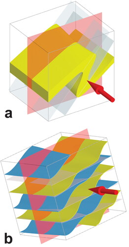
The symmetry axis of an object is an imaginary line that passes through the object and divides it into two mirror-image halves that are identical in shape and size. Geologically, this implies that there is a consistent continuity of grade or lithology along the symmetry axis (Figure 1).

Figure 1. Symmetry axis (red arrow) and orthogonal to this axis is the reflection symmetry plane (red plane) for (a) monoclinic fold and (b) C-S fabric. Geometries are independent of scale.

Resource geologists routinely use axial symmetry as a guide for creating estimation domains from drilling data, even though they may not be consciously aware of this process (it’s the well-worn habit of using cross-sections) (Cowan, 2016). The tradition of drilling on section planes was to allow sections to be hand-drawn and to make polygonal grade estimates of mineral deposits (Annels, 1991). In today’s computerised world, what exactly are we trying to achieve by continuing to interpret in cross-sections? To answer this, we need to clearly define a cross-section:

“A diagram or drawing that shows features transected by a given plane; specifically a vertical section drawn at right angles to the longer axis of a geologic feature, such as the trend of an orebody, the mean direction of flow of a stream, or the axis of a fossil” (American Geosciences Institute, 2023).

This definition specifically states that the cross-section is vertical, but it also states it must be drawn at right angles to the longer axis of a geologic feature. Thus, the formal definition of a cross-section is not only vertical but also a reflective symmetry plane across an axial geological feature.

We contend that the crucial aspect of defining a cross-section is not its orientation but rather its perpendicularity to a linear feature—that is, the section plane is a reflection plane perpendicular to an existing orthogonal axis. For example, in the case of a fold axis, the reflection plane is the fold profile (Figure 1a), and for a C-S fabric (Berthé et al., 1979), the profile plane is orthogonal to the intersection of C and S fabrics (Figure 1b). The rationale for using cross-sections in geological interpretation is not because of their vertical orientation; instead, it is because they can help rapidly interpret geological features from section to section. Because geological units and structural permeability are most continuous along this axis, the alteration, as well as grade, is also most continuous along this axis. Thus, the vertical sectional orientation itself does not contribute to producing an accurate interpretation of the geology, but the critical factor is the orientation of the section to a known geological feature, which must be visually identified by the geologist conducting the interpretation. Disregarding this seemingly minor step will result in inaccurate geological models, potentially leading to downgrades in Mineral Resource estimates. As indicated in the summary of the Phoenix deposit, this was cited as one of the major reasons for reducing that deposit’s Mineral Resource estimate.

We propose the intelligent use of axial symmetry in geological patterns that can be visually discerned from both grade and lithology in drilling data. By doing so, the degrees of freedom for modelling can be significantly reduced.

If we assume that the centroid of the deposit remains fixed at (x, y, z), the orientation degrees of freedom can be expressed by the three angles (φ, θ, and ψ) around the x-axis, y-axis and z-axis, respectively. Additionally, the ellipsoidal lengths (a ≥ b ≥ c) can be used to approximate the mineralisation, providing three more degrees of freedom that result in an infinite number of geometric fits. To simplify the modelling process, we can constrain our line of sight parallel to the axial symmetry and estimate the principal axial positions of b and c in the cross-sectional view perpendicular to the a-axis. Thus, we reduce the modelling problem to only three degrees of freedom, which is estimating the relative axial lengths of a, b and c of the best-fit ellipsoid. The same steps can be applied to multiple domains and lithologies without any modification, but the key step is to first identify the axial symmetry of the object to be modelled. The above steps are simple and give repeatable results even if achieved visually on screen (discussed in the next section).

For this reason, we believe that a ‘brute force’ modelling approach of generating multiple implicit geological models to document modelling uncertainty, such as that proposed by McManus et al. (2021), is inefficient and will likely result in many geologically inaccurate models as it fails to reduce the degrees of freedom of the modelling process. We contend that by considering axial symmetry, the modelling process can be limited to just three degrees of freedom, resulting in a small range of models—even a single model in the simplest of cases.

Various techniques are available to identify the axial symmetry of grade and lithological data, but a fast and effective visual method is using a simple computer projection technique developed for the medical industry during the early computer era—Maximum Intensity Projection, which was originally developed for analysing 3D computerised tomography data (Wallis et al., 1989).

Maximum Intensity Projection (MIP)

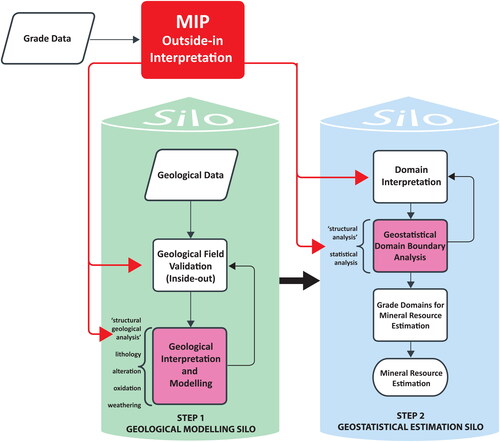
Prior to delving into MIP, it’s necessary to touch on where this ‘structural geological analysis’ fits into the resource estimation workflow (Figure 2). The term ‘structural geological analysis’, frequently shortened to ‘structural analysis’, does not equate to the ‘structural analysis’ of grade continuity that geostatisticians carry out as part of the grade continuity analysis utilising variography. Our structural analysis is conducted prior to the construction of domains and centres around determining the structural symmetry of grade distribution in geographic coordinates.

Figure 2. Resource modelling workflow is typically segmented into two largely independent workflows, visually represented as silos. Although we do not advocate this split, it is a common practice in the mining industry. The ‘structural analysis’ we are discussing with the use of MIP falls within the geological interpretation procedure, denoted in pink in the left-hand geological modelling silo. Conversely, the ‘structural analysis’ carried out by resource geologists slots into the geostatistical estimation workflow, depicted on the right, once again highlighted in pink. Ideally, insights derived from MIP can be utilised in both these processes, and even beyond, as depicted by the red arrows.

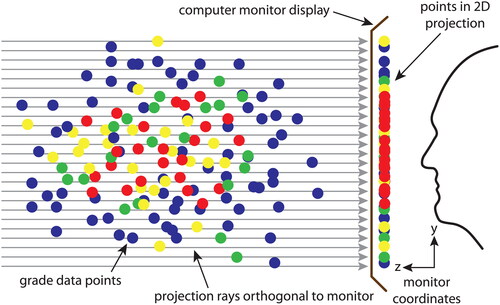
The visual analysis of grade data can be simplified by using the MIP rendering method, which involves projecting 3D point values into a 2D image using a ray orthogonal to the computer monitor plane (Figure 3).

Mineral deposits commonly comprise a core of high grades surrounded by a lower-grade halo (Figure 4), making it difficult to discern the deposit’s details. However, MIP can bring the highest value points forward along the ray in the projected 2D image, providing an X-ray view of the deposit. For the past two decades, we have used the MIP technique to efficiently analyse both dense and sparse drill-hole data on hundreds of mineral deposits (see examples illustrated in Cowan, 2014, 2020a). We have found that desurveyed mid-point data, which includes x, y, z and grade, is better suited for data interpretation than drill-hole interval data. By increasing the point size of assay points on screen, we can create simulated 3D volume data that do not require significant processing power or time. Combining MIP with the physical rotation of data into down-plunge view (Cowan, 2014; MacKin, 1950) allows geologists to determine the linear grade alignment in sparse assays sampled with drill holes.

Figure 3. Schematic cross-sectional view of a computer monitor showing how MIP works with grade point data. The highest grade point values from the cloud of grade data are projected to the front of the computer monitor along a path orthogonal to the monitor.

To illustrate the usefulness of MIP, synthetic data representing a cylindrical fold object with a finite thickness (Figure 4a) was created from a drawn fold mesh (Figure 4i) to train geologists in this technique. The objective was to model the boundary between the ore and waste zones as quickly and accurately as possible. The MIP technique was used to reveal the fold profile view, and the geologists were quickly able to determine the geometry of the ore body. Although the MIP view is 2D, the primary 3D point dataset can be rotated to find a distinctive fold profile pattern (Figure 4a–c). Between 2003 and 2012, Jun Cowan conducted this exercise during geological modelling training sessions that involved hundreds of geologists with varying degrees of experience. In each session, the geologists were able to replicate the down-plunge orientation within a cone of approximately 5°.

Figure 4. Synthetic grade dataset with ‘ore’ in red and ‘waste’ in blue: (a) low grades surround the high grade so the geometry of the ore cannot be deciphered easily; (b) MIP on an arbitrary viewing direction yields nothing that is geologically sensible; (c) only the down-plunge orientation reveals a fold profile; (d–h) MIP rendered vertical sections parallel to the drilling fence, but these sections display ill-defined 2D continuities across three fences, failing to reveal the true 3D geometry of the ore as these sections are not orthogonal to the symmetry axis of the ore body; (i) original fold-shaped mesh object used to create the data; (j) ore boundary is modelled by first identifying the axial symmetry orientation from the data points; and (k) model resulting from isotropic interpolation of data ignoring axial symmetry orientation.

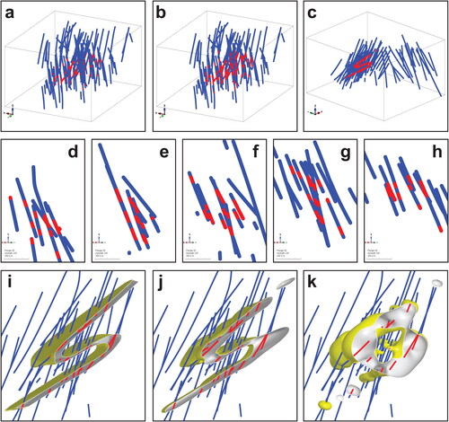
In contrast, vertical sections (Figure 4d–h), which are not orthogonal to the symmetry axis of the data, result in confusing and commonly conflicting apparent 2D continuities even with this simple fold-form geometry (Figure 4i). Interpreting in vertical sections, which is standard practice in the mining industry, is not recommended unless the section is orthogonal to the continuity direction.

Using the visually estimated principal directions of the simulated ore distribution, implicit modelling of the data can be performed quickly and accurately, as shown in Figure 4j. This method allows multiple geologists to generate models with similar axial symmetries without the need for time-consuming sectional digitisation. The exercise involving MIP and implicit modelling usually takes only a few minutes and because the fold axis and axial plane can be accurately identified and replicated by multiple geologists, the resulting models are highly reproducible and nearly identical, greatly improving modelling speed and reproducibility. A model created using traditional modelling methods, where each section is digitised by hand, cannot match the accuracy of the model depicted in Figure 4j because there is no assurance that the vertical sections used for interpretation will be orthogonal to the axial symmetry of the mineralisation.

However, it is not advisable to depend solely on isotropic implicit models, as proposed by Stenhouse et al. (2020, figure 6), without analysing the raw grade point data to identify the axial symmetry orientation. This is because the results obtained through interpolated modelling are strongly influenced by both the values being interpolated and their spatial sampling locations. An isotopically interpolated model of the data depicted in Figure 4a–c is shown in Figure 4k, which does not resemble the synthetic model of Figure 4i.

To further illustrate the impact of sampling bias on implicit modelling, another synthetic model was created based on an exercise presented in Turner and Weiss (1963, figure 5-12), featuring two lithologies with a folded interface (Figure 5). As depicted in Figure 6, three groups of models were produced from 11 sets of drill sampling of the synthetic model. One set was sampled using the traditional fence drilling method, which was sampled across strike, while the other 10 sets were randomly oriented. The models in Series 1 were created using isotropic linear interpolation, which is the default setting in Leapfrog software. The highly variable results displayed in Series 1 clearly demonstrate that different sampling patterns can produce significantly different outcomes from identical lithological distributions. Depending solely on these outcomes can lead to a wide range of geological interpretations that are largely influenced by the drill sampling pattern.

Figure 5. Synthetic two-lithology geological model created using an exercise in Turner and Weiss (1963, figure 5-12): (a) is the model with the original map overlay of a down-plunge exercise, and (b) the synthetic model. This synthetic model was sampled by virtual drill holes of various orientations and positions as shown in Figure 6.

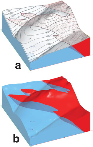
Figure 6. Synthetic model of Figure 5 sampled and modelled with fence drilling and 10 other random drill sampling methods, two of which are shown here. Top row (Series 1) represents isotropic interpolation just using drill-hole data. Middle row (Series 2) is the result of the same isotropic interpolation with the contact of the two lithologies digitised in plan. Bottom row (Series 3) includes the contact of the two lithologies and was modelled with an imposed anisotropy with the maximum axis of the ellipsoid parallel to the down-plunge and a–b plane of the triaxial ellipsoid parallel to the axial plane of the folded interface. See animated GIF file in supplemental data showing all models for each series of models.

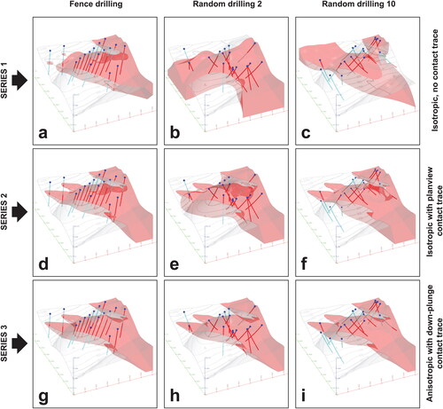
Figure 7. (a) Horizontal sectional slice located at the base of the synthetic model shown in Figure 5. The traces of the 11 models produced for Series 1, 2 and 3 are displayed in (b), (c) and (d), respectively. The arrow in the figure indicates the trace of the lithological contact from the synthetic model (a); all drill-hole segments are depicted in these sections.

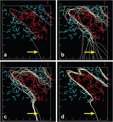
Figure 8. Box plot of the modelled volume of the red unit in Series 1, 2 and 3, compared with the true volume of the red unit in Figure 5b (dashed line). Each series represents 11 modelling realisations from 11 sets of drill patterns. The box in the plot represents the interquartile range. The white line in the box is the median, and ‘x’ is the mean value. The vertical axis is in volumetric units.

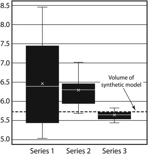
Figure 9. Simplified geological plan after Gartz (2008). The location of the study area is marked with a red box, both on the location plan and on the map. The study area is located in the Meekatharra–Wydgee Greenstone Belt in the NE Murchison Province of Western Australia.

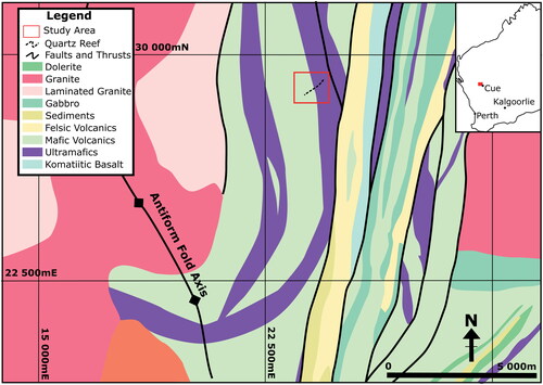
Figure 10. Simple workflow outlining the basic processes involved in building a robust structural model from grade data. Figures 11, 12 and 13 describe a simple process that can acquire useful structural information from the grade data.

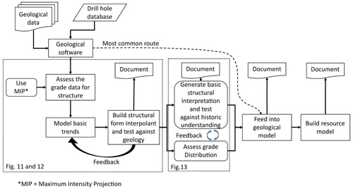
Figure 11. Simple workflow using MIP to analyse a deposit. (a) View with gold projected using MIP looking down plunge at 48→117. (b) An apparent fold is identified in the gold data. (c) The gold trend has been modelled using a series of structural discs (MIP turned off for clarity). (d) A series of structural forms have been modelled based on this structural geological data that model the fold surface. (e) The form surfaces are compared against the gold to see if the trends still make sense looking down plunge. (f) The same down-plunge view but showing the extracted volume points for the porphyry unit (in red). (g) A stereonet of the structural discs shows the poles form a great circle with a pole plunging SE at 48→117. (h) The fold trends overlayed onto the regional geology looking down the plunge of the apparent fold axis. Legend: Au g/t is the gold composites in grams per tonne, Porph is the porphyry, Disc means the structural discs, Forms are the structural forms built from the grade composites and fold is the interpreted fold seen in the grade.

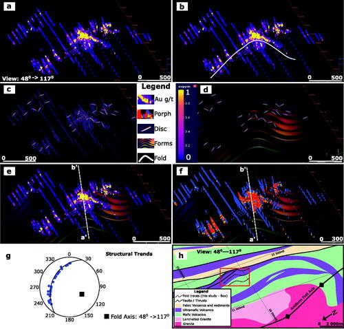
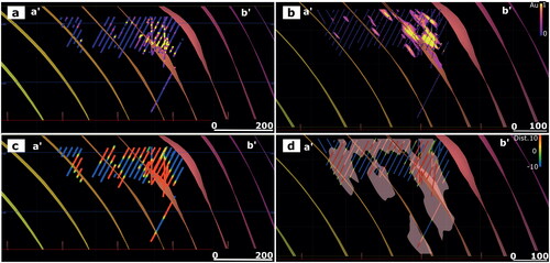
Figure 12. Form surfaces assessed in section looking NE along the fold axial plane (a′–b′ in Figure 11e); refer to Figure 11 for the legend. (a) The plunge of the grade was assessed against the form surfaces. (b) A series of grade shells were created using a structural trend based on the form surfaces to drive the implicit modelling interpolant. (c) The porphyry is compared against the grade-based fold trends; the porphyry volume is shown (in red). (d) A porphyry wireframe model was generated using the form-surface trend model to drive the interpolation.

In Figure 6, Series 2 shows the same isotropic interpolation setting as Series 1, but with the addition of the surface contact trace between the two rock units, digitised in plan view. In Series 3, 11 models were generated that are minimally affected by the drilling pattern, which includes the contact trace, digitised viewing along the plunge axis, as well as the estimated anisotropy. The models produced in Series 3 are almost identical, regardless of the sampling pattern, and use the same drilling patterns displayed in Series 1 and 2. Figure 7 displays the deviation of the model contacts resulting from the three modelling methods at a depth significantly away from the digitised surface contact trace. These experiments reveal that isotropic interpolation yields highly variable results depending on the drill sampling (Figure 7b, c) and cannot be considered ‘unbiased’ as claimed by Stenhouse et al. (2020). The isotropic modelling of Series 1 resulted in the largest volume variations as well as an overestimate of the average volume (Figure 8). Series 2 performed comparatively well and appeared realistic, yet it still overestimated the volume when compared with Series 3, which incorporated anisotropy into the interpolation, aligning it with the structural shape of the plunging fold. The complete set of drill sampling and resulting models from the experiment depicted in Figure 6 is available as an animated GIF file in the Supplemental data.

An isotropic implicit modelling approach that is blind or ‘black-box’ in nature can be severely limited and may prove to be costly as it may not uncover structural geometry, even when the dataset is perfectly constructed (Figures 5–8; Supplemental data). Therefore, traditional explicit methods of digitisation performed on sections that are orthogonal to the axial symmetry line of the mineralisation are likely to produce superior results compared with a blind implicit modelling approach that disregards structural geometry.

Digitisation method of 3D planar continuity

The modelling technique shown in Figure 6g–i and 7d (Series 3) involves a specific digitisation method. It operates on the principle of measuring bedding in an inaccessible cliff face by walking to a position where the viewer is aligned with the strike line of the bedding. From this viewpoint, they can look along the strike and measure a true dip value because the view is confined within the bedding plane.

The method of measuring the tangent plane using a 3D viewer is not restricted to the strike-line view alone. It is possible to view the plane of continuity along infinite lines, not just the strike line. The optimal approach involves digitising the local tangent plane by viewing along the rotational symmetry line of the surface being analysed. Conventional compasses and digital phones cannot achieve this type of measurement in the field. However, the digitising tool in Leapfrog software was specifically developed by Jun Cowan to enable this type of measurement. For instance, when analysing a folded surface, the viewer needs to look along the fold axis to digitise tangent planes. With the aid of MIP projection, grade trends along the bedding become clear when viewed along the line of symmetry, and it is possible to determine if the view line is within the local tangent plane. This allows digitisation of tangent planes in a down-plunge projection view, as demonstrated in a case study below.

Building a simple structural model for geology and resource modelling—a case study

It is crucial to comprehensively understand and evaluate the underlying structural geological controls when building a geological model for resource modelling purposes. This involves using all available data and directly incorporating the knowledge of the geologists who conducted the mapping and drill-hole logging to ensure the resulting resource model is robust. Regrettably, many projects lack fundamental knowledge and understanding of structural geology, and in many cases, the basic structural geological data are not collected. Within the mining industry it is also common to review a historic dataset or an old mine to reassess a project for additional mineralisation that may have been missed in the past—in such cases a comprehensive dataset may be lacking.

Where structural geological data are unavailable, the grade data can be used to gain a basic understanding of the structural controls of a deposit, as discussed above and detailed by Cowan (2014, 2020a). The workflow allows the modeller to form a basic structural geological framework from the grade data and build a testable model using the ‘outside-in’ method of analysis, as discussed by Cowan (2020a, 2022). This model can then be tested against other available exploration data (e.g. geological mapping, drilling, core photos and other forms of data). Data should be assessed critically, hypotheses re-evaluated in light of new or additional data (Vann & Stewart, 2011), and, where possible, reference should be made back to the geology. Building upon this foundational knowledge, a sound geological model with a structural framework can be established and used to inform resource estimation.

The project discussed in this case study is a small gold deposit in the Meekatharra–Wydgee Greenstone Belt in the NE Murchison Province of Western Australia (Gartz, 2008). Internal Harmony Gold Mineral Resource reports describe the deposit as comprising a mineralised quartz vein cutting porphyritic granodiorite intrusions. The deposit is hosted by north–south–trending, multiply deformed, intercalated, high-Mg mafic and ultramafic volcanic rocks containing minor interbedded felsic volcanic and sedimentary units on the east limb of a south-plunging granite-cored antiform (Figure 9). The area has been metamorphosed to amphibolite facies and intruded by several granite bodies, some of which show strong foliation development. Several east-over-west thrusts cut the stratigraphy and truncate the mineralisation, and some porphyritic granodiorite dykes with strongly foliated contacts intrude into the area.

The main mineralising event comprises quartz veins within the porphyries, particularly around the edges of the porphyry bodies, with strong silica–sericite–sulfide alteration near the mineralisation. A significant quartz reef with very high grades cuts the study area. In the past, miners targeted this reef using small shafts and drives to access the upper levels of the quartz reef. This quartz reef is the main fluid conduit for mineralisation, it is well mapped and is the main basis for the original resource domain wireframes.

The approach here is to accept the presence of the reef but filter it from the review of the historical data to see what additional working hypotheses can be developed. A difficulty faced by many geologists is stepping outside their usual perspective and practices to view and examine the geologic and drill data afresh (Vann & Stewart, 2011). The ‘fact’ that the quartz reef is the source of the mineralisation can be considered the consensus view. By removing it from consideration, we can assess the data from new and unique perspectives.

A modelling workflow is presented in Figure 10 that gleans some structural information from the grade data to build a testable underlying structural model. A reading of Mineral Resource technical reports shows that the most common route followed after loading data into the software is to generate a geology model (or occasionally go straight to building the resource model), effectively bypassing the structural assessment stage. Unfortunately, many modellers miss the significant portion of work involved in constructing the structural framework—the skeleton of the geological model. Structural modelling has two major components: (1) hypothesis building and testing (Figures 11 and 12) and (2) model finalisation and validation (Figure 13). Both should be completed before creating a model of the deposit geology or resource estimation domains. This process can also be used to assess the resource estimation domains constructed by someone else as part of an internal peer review process or perhaps as a potential business opportunity.

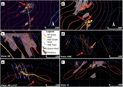
Figure 13. (a) Two assumed structures based on the grade shells are shown in yellow and white. The red arrow indicates a structure that seems to be quite significant. (b) The original domain wireframes (orange) are comparable with the grade shell (red) and the porphyry (brown). The red arrow indicates the location of the interpreted fault in (a). (c) The original interpretation appears to be similar to the newly modelled grade domain and the structural form surfaces. (d) The original wireframes (red arrow) assume a much steeper dip than shown by the form surfaces; the original reef wireframe is marked with the orange arrow. (e) The potential for additional metal in the pit wall (red circles) was not targeted because the original grade wireframe dips away from the grade trends (red arrow). (f) Several potential exploration targets were missed. IM, Implicit Model; RSO, Original resource domains; ASB, post-mining surveyed As-Built topography.

Figures 11, 12 and 13 demonstrate how to evaluate and model the fundamental structure of a deposit using only grade data at the deposit-scale. Assessing the grade data independently of other information has a significant advantage in constructing new and verifiable hypotheses. The grade is generally influenced by the underlying geology (such as rock types, alteration and structures), and the patterns observed in the data commonly reveal the story of the mineralising event. After developing a structural hypothesis based on the grade data, the model’s characteristics can be compared with historical literature, field or pit mapping data, and the accuracy of the interpretations can be evaluated. By using MIP to modify the colour spectrums of the grade values, it is possible to accentuate various underlying geological controls. For example, a low-grade halo might be controlled by a specific rock type, while high grades may be controlled by a foliation fabric. If MIP is not available in the software, creating a series of grade indicators with contrasting colours and sizes for two grade bins can achieve a similar outcome, albeit with greater difficulty (Barnes & Gossage, 2014).

Workflow

Using MIP to display the grade data simplifies the process of determining the axial direction with the greatest linear continuity of the mineralisation. Rotating the data on the computer monitor causes the linear trends to converge to a point at a particular orientation, much like observing the end of a pencil after rotating it. This orientation corresponds to the axial symmetry and is equivalent to the down-plunge axis. In the case study, the projected area of the high grades appears to be the smallest when viewed at 48→117, indicating that this is likely the down-plunge orientation (Figure 11a). This particular viewpoint seems to define a folded profile that may indicate lithological controls on the gold (Figure 11b). It is important to note that this does not necessarily suggest that the mineralisation existed before folding occurred; rather, that the underlying host rock may be folded. This allows us to generate a simple hypothesis that the host to the gold appears to be folded, and this is further investigated below.

An understanding of the folded trends becomes evident by digitising local tangents (in this case as structural discs) to the curvilinear grade traces in the down-plunge view of grade (48→117) using MIP rendering (note that in Figure 11c, MIP is turned off for clarity to see the structural discs). Sufficient structural discs have been digitised to define the planar tangents to the grade patterns and used to build a structural form-surface model (Figure 11d). Comparing these form surfaces with the original grade data (Figure 12a) is important for validation but also helps to identify other significant trends. Additionally, this method can be used to model other controls on mineralisation resulting from discontinuities, such as shears and faults. These trends are digitised using a drawing tool and added to the interpretations and the model. Structural discs, which can be used to define tangent planes, are a feature of some software products. If this feature is not available, trend-based polylines can be digitised on the screen viewing down plunge to achieve a similar result and allow the overall structure to be visualised.

Figure 11e displays the grade data looking down plunge, viewed at 48→117, while Figure 11f displays the logged porphyry intersections from drilling. The porphyry units appear to conform to the fold patterns seen in the grade data. In this case, the porphyry lithology has been extracted from the drill-hole data and displayed as points inside (red) and outside the porphyry (blue). Some software products can generate these points directly from drilling interval data, or they can be created manually using a spreadsheet. To create the points manually, first composite the lithology data into equal lengths and desurvey it to x, y, z lithology tables. Then, in the spreadsheet, points inside and outside the lithology of interest can be assigned values of +1 and −1, respectively, while contact points can be assigned a value of 0. Combining these two files and loading them into the viewer allows the porphyry trends to be evaluated using MIP in the same manner as the grade. The red points inside the porphyry have a higher value, so they take precedence over the points lying outside the porphyry when viewed with MIP. By examining the porphyry data in this way, potential faults and shear zones, as well as other controls, may become more evident. At this stage, a hypothesis can be formed that the broad grade distribution appears to be controlled by folded lithological units. However, this hypothesis should be validated against other independent geological information, as it was developed solely based on the underlying patterns observed in the grade distribution without any input from other geological data.

Figure 12a looks NE, normal to the apparent fold axial plane, while Figure 12b shows grade contours created using implicit modelling as influenced by the form surfaces, which we refer to as ‘form-surface trends’. The grade generates coherent bodies that can be used to drive resource domaining decisions. Some software programs allow for modelling 3D grade contours that follow the form surfaces generated in the previous step using a form-surface trend model (Figure 11d). However, as of 2023, no software is available that allows modelling of triaxial continuities along these form-surface trends. Instead, oblate continuity along the form surfaces is currently the only option, which can lead to inaccurate results but can still serve as an approximate guide. If the software does not allow for the construction of form interpolants and form-surface-based grade models, similar results can be achieved using a series of simple wireframes representing grade envelopes. These can be manually generated by digitising polylines (strings) on down-plunge sections by following the form-surface trends. With care, this approach can yield better results than automated methods because the down-plunge continuities can be taken into account. In Figure 12c, a comparison is presented between the form surfaces generated from the grade-based data and the logged porphyry data, which also appears to follow the form surfaces. The figure indicates a discernible link between the form-surface trends identified from the grade and the volume of porphyry points. This close correlation suggests an apparent association between the gold, the porphyry and the folding. The grade-based form-surface trend model was then used to build a 3D porphyry model based on the porphyry logs (Figure 12d). In this case, the structural model defines what appears to be significant folding that has possibly affected the mineralisation host rocks, including the porphyry (as shown in Figure 11). This step establishes a further geological control to the grade distribution that can be checked against the core and may be used in the resource domaining process rather than simply relying on an assumed grade cutoff value.

The model was tested against the known local and regional geology. A structural model should not be an isolated entity—it should reflect a small component of the larger whole. In the case study, the deposit sits on a regional-scale fold, and the fold contours constructed from the grade are a good match against the stratigraphy in the regional geology maps. Figure 11g shows a stereonet of the structural discs created in Figure 11c; they plot on a great circle with a plunge axis of 48→117. Figure 11h shows the regional geology looking down the plunge described in Figure 11g and confirms that the fold trends are on the eastern flank of a regional SE-plunging antiform.

According to a production report (Pinder, 2007), the mine experienced notable ore reconciliation problems during mining. Table 1 summarises the close-out reconciliation reported during a significant cutback operation in 2005. It is possible that the insufficient identification and modelling of porphyry mineralisation and folded controls, as observed in this study, could account for the unsatisfactory reconciliation results.

Table 1. Reconciliation figures for a significant cutback on the pit, based on the end of mine reconciliation report (Pinder, 2007).

	Tonnes	Au g/t	Ounces Au	Diff.T to RM	Diff.Au to RM	Diff.Oz to RM
Resource model (RM)	84 185	4.56	12 345
Grade Control model (GCM)	94 073	4.27	12 908	112%	94%	105%
Actual Credited (AC)	136 196	3.04	13 329	162%	67%	108%

Once a relationship between the stratigraphy/geology and the gold has been established, possible target areas can be assessed for future drilling. Figure 13 uses grade shells to enhance clarity and reveals the presence of two potential fault structures that appear to intersect with the mineralised lenses (as shown in Figure 13a). These faults have a notable impact on the grade model and should be visible in the pit wall and previous domain interpretations (as depicted in Figure 13b). It is always advisable to verify the existence of these structures by examining drill core (or the core photos), surface mapping, and pit/underground maps, if available. Given their significance from a resource perspective, it is likely that these structures should have been included in the original modelling.

Figure 13b depicts the grade shell (outlined in red) and the porphyry model (in pale brown) alongside the original resource domains (in yellow). The previous grade-based resource domains were explicitly modelled in 2D, in plan and cross-section, perpendicular to the quartz reef and the assumed mineralisation strike. The implicitly modelled shells align with the general trend of the original resource grade shells in plan. Additionally, the possible structures highlighted in Figure 13a coincide with some of the breaks in the original estimation domain model, as well as some of the previously interpreted lodes and faults. As a result, it appears that these structures were identified in the past and have some basis in the data. Notably, the as-built mesh of the completed mine, designed around the quartz reef, aligns with the folded trend, indicating that there may have been an understanding of a relationship between the folded stratigraphy and the distribution of grades. However, none of the available reports appear to have discussed this connection.

Assessing the models in section helps validate the robustness of the existing wireframes to see whether the original domain geometry matches the understandings developed in the new modelling. Figure 13c looks in the same NE section normal to the fold axial plane, as seen in Figure 12a. The old domain shell adequately matches the grade shell taken from the implicit model and also matches the porphyry model. In contrast, when assessed in the original ENE-looking mine grid section, there is a significant mismatch between the original resource domains and the newer model (Figure 13d). The implicit grade model built using the folded grade trends, and the porphyry model, seem to dip at a lower angle than the original sectional interpretation. The original wireframes assumed the grade is contained in and around the quartz reef; however, the grade can be seen in the drilling in Figure 13d to have the same dip as the interpolated grade contours and not the steep orientation seen in the original domain model. It appears that the reef may not have the steep dip indicated by the resource domain wireframes, and perhaps this may have been a cause of the poor reconciliation.

This departure of the original model from the grade trends modelled here is apparent when assessing the data viewing down the fold plunge (Figure 13e). The quartz reef domain was remodelled from drilling using the understandings from this study—it has a lower-angle dip than the original interpretation and intersects one of the potential target zones. This grade interpretation implies a doubly plunging distribution following the fold trends seen in the porphyry and bedding. As the explicit interpretation was driven solely by the quartz reef, it indicates only a single plunge direction based on the expected dip of the shear, which deviates from the updated understanding of grade distribution. Although the shear and quartz reef are real features, the underlying grade patterns are potentially strongly controlled by the bedding and the porphyry dykes or sills. This indicates that two porphyry-based exploration targets may have been missed. Here, explicit model domains based on the assumption that the quartz reef controls gold distribution do not match the understanding of the mineralisation developed by analysing the grade data. The quartz reef undoubtedly contains gold, but it is not the only control on mineralisation in the deposit.

With improved understanding of the distribution of grades and potential lithological influences, exploration efforts can now begin to seek extensions to the mineralised porphyry, mineralised shears and quartz reef. Figure 13f, a section parallel to the yellow fault in Figure 13a, highlights numerous promising targets for grade, both shallow and deep, that can be further explored in future drilling campaigns; all were missed, including potential reef extensions, owing to the rigid 2D sectional interpretation methodology used in constructing the original domains and geological models.

Following the modelling process described above may raise questions and reveal additional complications. For example, in this case study, the original internal resource and geology report discusses “significant schistosity in the rocks that is more prevalent in the Ultramafics…”. Because the porphyry is a likely gold host and appears folded, assuming it was emplaced before folding, it may be foliated as well. It is possible that the schistosity corresponds to an axial plane foliation, but the lack of structural measurements of foliations in the historical data and the absence of any documentation of the schistosity make it challenging to verify its relationship to folding or its relationship to the gold distribution. The importance of the schistosity in terms of controlling mineralisation highlights the need for it to be recognised, recorded and assessed.

Discussion

The case study above illustrates how structural geological analysis of a mineral deposit at the deposit-scale can provide valuable insights that can be field tested, and highlight potential areas for further exploration and mining opportunities. Structural interpretation based solely on assay data is not a common practice, but it is crucial to recognise that such non-traditional techniques can open up a new range of observations and opportunities. However, this shift in perspective requires breaking away from entrenched mining industry practices that are based on operational needs and the constraints posed by presently available analytical techniques rather than on scientific validity. These entrenched practices include: (1) persisting with established mining industry practices, such as fence drilling, the use of mine grids and vertical section interpretation; (2) relying on default implicit software settings and inadequate training for geological modelling that ignores deposit-scale structural geology and object symmetry; (3) extrapolating observations from the field-scale to the deposit-scale (inside-out), rather than validating predictions by first analysing deposit-scale grade patterns (outside-in); and (4) rigidly adhering to established geostatistical conventions, such as analysing grade continuity through variography, which may overlook the structural context that is revealed through MIP.

For example, geostatisticians typically focus on intra-domain axial symmetry, as seen in the maximum grade continuity axis derived from variography, which is familiar to resource geologists. However, the interrelationships between different domains are rarely examined. As a result, geostatisticians, for example, may be unaware of the structural patterns that could be easily observed on their computer screens if they were to consider this perspective.

A similar level of ignorance occurs at the larger scale, caused by the use of the mine grid, where individual mineral deposits in a mining camp are assigned separate coordinates and because of the established habits of the mining industry these grids are rarely examined together (Cowan, 2020b). One straightforward example of this is the domaining of a fold-hosted mineral deposit into three volumes: the fold hinge and the two limbs of the fold. Each volume has a unique grade continuity defined by variography. Although necessary for geostatistical resource estimation that relies on the current paradigm of rectilinear estimation methods, these domains are not a natural feature of the mineral deposit but rather an artificial construct created in an attempt to define volumes of geostatistically stable grade characteristics, e.g. stationarity, that underpin estimation methodologies. From a scientific standpoint, these domains are essentially useless in understanding the mineral deposit and may hinder our ability to understand the deposit’s structure. Scientifically, examining the structural interconnection between domains provides valuable insights into the structural influence on mineral deposits. We believe that understanding this science can lead to improved decision-making concerning the exploration, modelling and extraction of Mineral Resources.

The mining industry’s habit of relying on vertical sections to interpret geological data from drilling is concerning and may have led to unintended consequences, especially when the symmetry axis is not orthogonal to these sections (Figure 4d–h; Cowan, 2016). This approach can lead to invalid assumptions of grade continuity being built into the modelling process. Although vertical sections reduce the rotational degrees of freedom, they are commonly at the wrong orientation and placing emphasis on these sections can result in significant Mineral Resource estimate downgrades. The Phoenix deposit provides a notable case in point, but we suspect the prevalent practice of using vertical cross-sections is a common reason for resource downgrades.

Rapid implicit modelling, which has so many benefits, may result in worse resource estimation results than more traditional and slower methods of explicit modelling. Over the last decade, there has been an increasing reliance on implicit modelling software’s default settings to create geological and Mineral Resource estimation domains without properly specifying appropriate constraints. This practice poses a significant risk because these volumes are highly sensitive to drill sample orientation and density, as evidenced in our experiment (Figures 5–8). Regrettably, this is an unintended consequence of the rapid adoption of this modelling technique without providing adequate and necessary user training. Inadequate (or no) training means that users cannot recognise and use structural symmetry patterns intelligently, which will lead to persistent overestimation of domain volumes and thus increase the chances of unforeseen Mineral Resource downgrades. Instead of generating numerous implicit geological models to try and capture uncertainty (as suggested by McManus et al., 2021), we advocate for the smart application of axial symmetry in geological patterns—patterns can be visually identified from drilling data in both grade and lithology. By doing so, the degrees of freedom for modelling can be significantly reduced. Orientation represents three degrees of freedom, and ellipsoidal lengths provide an additional three degrees of freedom that can approximate geological features. By limiting our view line aided by axial symmetry, we can effectively reduce the modelling process to only three degrees of freedom. Any deviation from the axial direction would be geologically infeasible. As demonstrated by Stoch et al. (2022), a brute force method of modelling will overstate the uncertainty in the geological model and skew the results of the resource estimation. We argue that this can be avoided by considering axial symmetry a mineral deposit, and a smaller range of models can be generated within just the three degrees of freedom offered by the ellipsoidal fit.

Industry professionals need to understand that the non-scientific operational habits discussed above have had unintended consequences on the understanding of mineral deposits over the last 70 years. For example, the structural understanding of mineral deposits that was common knowledge in the mid-20th century has declined significantly (Canadian Institute of Mining and Metallurgy, 1948, 1957; McKinstry, 1948, 1955; Newhouse, 1942). We believe that these non-scientific operational habits have contributed to a decline in the geological understanding of mineral deposits within the mining industry since the 1950s.

Conclusions

Geological modelling for Mineral Resource estimation is not just a straightforward exercise in geometric shape modelling, as many professionals and software makers assume. Rather, it is an exercise in fundamental structural geological analysis (Cowan, 2017). Since the late 1950s, the Mineral Resource estimation process has largely overlooked structural geological factors, but it is illogical to suggest methods to quantify resource modelling uncertainty without taking structural architecture into account. A thorough understanding of the geological and structural aspects at the deposit-scale is crucial to developing sound Mineral Resource estimates—otherwise, there is a risk of significant estimate downgrades.

The deposit-scale structural model serves as the foundation for the geological and Mineral Resource models and is vital in ensuring that the resource estimation is as representative as possible. Although the inputs and insights of geologists in the field, including maps, logs, and imagery, are crucial for Mineral Resource models, they may not always be available. In such cases, a deposit-scale structural model can still be generated by analysing the grade distribution of the deposit using MIP. The authors are of the opinion that the outside-in MIP modelling methodology, as described here and by Cowan (2020a), should be an essential component of any resource domaining project. We conclude with nine key ideas to consider when applying this methodology of structural geological analysis to Mineral Resource estimation:

1. Apply the ‘outside-in’ deposit-scale structural geological analysis at all deposits irrespective of structural geological data availability. Structural interpretation of grade using MIP can form the structural context and small-scale predictions can be made, which can be tested in the field.

2. Avoid using vertical cross-sections unless they are parallel to the reflection plane of the geological feature of interest. It is crucial to identify the axial symmetry and use the reflection plane of that axis—commonly they are not vertical.

3. Do not depend solely on variograms to determine geological controls because they are not viewed and modelled in real world coordinates. Instead, visually estimate grade continuity at the deposit-scale using MIP as that will highlight the structural controls.

4. Consider not drilling along fences (may result in biased interpretation).

5. Do not be restricted by an imposed local mining grid as that may narrow your field of structural interpretation.

6. Do not interpret isotropic default interpolation outputs of grade or lithological data from implicit modelling software—they are highly biased and inappropriate for geological interpretation. Instead, interpret raw sampled data at the deposit-scale using MIP.

7. Use basic geological first principles to develop multiple geologically valid hypotheses and test them against the data.

8. Approach structural modelling from a whole of deposit starting-point using raw drill-sampled data and work from the outside (outside-in) rather than focusing on the details and extrapolating these to the deposit as a whole (inside-out).

9. Do not create multiple resource models to evaluate unconstrained uncertainty as this is highly inefficient, costly and may over-represent the real uncertainty. Instead, we suggest reducing the degrees of freedom by identifying the symmetry axes controlled by structural geometries, thus allowing a small range of models to be considered within that structural framework.

This study aims to assist resource geologists by proposing a path toward quantifying the uncertainty associated with geological modelling given our suspicion that it may contribute significantly to the majority of unexpected Mineral Resource estimation downgrades. However, the lack of publicly available data prevents us from independently verifying our hypothesis. To identify the root causes of major Mineral Resource downgrades with confidence, an independent investigation modelled after the aviation industry’s accident investigation process is necessary. We recommend the establishment of an industry-based committee of peers that can initiate an impartial enquiry into the causes of all significant Mineral Resource downgrades to enhance the mining industry’s credibility.

Acknowledgements

Our gratitude goes to Harmony Gold for allowing us to present and subsequently release this piece of work. We also appreciate the valuable feedback provided by Marat Abzalov and the insightful and constructive reviews by René Sterk, Stuart Masters, Chris Bonson and Julian Vearncombe, which significantly enhanced the quality of the paper.

Disclosure statement

No potential conflict of interest was reported by the authors.

Data availability statement

Data used in this study are Commercial-in-Confidence and not available for public release.

Additional information

Funding

This research received no grants from any funding agency in the public, commercial or not-for-profit sectors.

Notes

1 Throughout the text, we have capitalised the terms when referring to a Mineral Resource or Ore Reserve as a defined term under the JORC code (JORC, 2012). However, the terms resource and resource estimation are not capitalised when referring to the process of generating a Resource.

References

- Abzalov, M. (2016). Applied mining geology (1st ed.). Springer International Publishing.
- American Geosciences Institute (2023). Cross section. In Glossary of Geology. https://www.americangeosciences.org/pubs/glossary
- Annels, A. (1991). Mineral deposit evaluation: A practical approach. (1st ed.). Chapman & Hall.
- Barnes, J. F. H., & Gossage, B. L. (2014). The do’s and don’ts of geological and grade boundary models and what you can do about it. In AusIMM (Ed.), Mineral Resource and Ore Reserve Estimation; The AusIMM guide to good practice. Monograph 30 (2nd ed., pp. 175–188). The Australasian Institute of Mining and Metallurgy.
- Bernier, S., Cole, G., Hewitt, D., Taylor, S., Roy, P. (2014). Preliminary economic assessment for the F2 gold system, Phoenix Gold Project, Red Lake, Ontario (p. 264) [NI 43-101]. Rubicon Minerals Corporation. https://digigeodatareports.b-cdn.net/3443.pdf
- Bernier, S., Cole, G., Ravenelle, J-F., O’Flaherty, M., Frostiak, J. W. (2016). Technical report for the Phoenix Gold project, Red Lake, Ontario (p. 221) [NI 43-101]. Rubicon Minerals Corporation. https://www.miningdataonline.com/reports/Phoenix_Technical_02252016.pdf
- Berthé, D., Choukroune, P., & Jegouzo, P. (1979). Orthogneiss, mylonite and non coaxial deformation of granites: The example of the South Armorican Shear Zone. Journal of Structural Geology, 1(1), 31–42. https://doi.org/10.1016/0191-8141(79)90019-1
- Blenkinsop, T. G., & Doyle, M. G. (2010). A method for measuring the orientations of planar structures in cut core. Journal of Structural Geology, 32(6), 741–745. https://doi.org/10.1016/j.jsg.2010.04.011
- Briggs, M. (2017). Twin Bonanza—Buccaneer Resource update (p. 39) [Media release]. ABM Resources NL. https://wcsecure.weblink.com.au/pdf/ABU/01891650.pdf
- Canadian Institute of Mining, Metallurgy and Petroleum. (2022). Canadian Securities regulatory standards for mineral projects. Standards, Best Practices & Guidance for Mineral Resources & Mineral Reserves. https://mrmr.cim.org/en/standards/canadian-securities-regulatory-standards-for-mineral-projects/
- Canadian Institute of Mining and Metallurgy. (1948). Structural geology of Canadian ore deposits, A symposium arranged by a committee of the Geology Division, Canadian Institute of Mining and Metallurgy. Canadian Institute of Mining and Metallurgy.
- Canadian Institute of Mining and Metallurgy. (1957). Structural geology of Canadian ore deposits, a symposium arranged by a committee of the Geology Division, Canadian Institute of Mining and Metallurgy. Canadian Institute of Mining and Metallurgy.
- Coombes, J. (2008). The Art and Science of Resource Estimation. A practical guide of geologists and engineers. Coombes Capability. www.coombescapability.com.au
- Cowan, E. J. (2014). X-ray plunge projection’—Understanding structural geology from grade data. In AusIMM (Ed.), Mineral Resource and ore reserve estimation; The AusIMM guide to good practice. monograph 30 (2nd ed., pp. 207–220). The Australasian Institute of Mining and Metallurgy. https://www.researchgate.net/publication/281685742_'X-ray_Plunge_Projection’-_Understanding_Structural_Geology_from_Grade_Data
- Cowan, E. J. (2016). Why I give geological cross-sections the cold shoulder. LinkedIn. https://www.linkedin.com/pulse/why-i-give-geological-cross-sections-cold-shoulder-jun-cowan/
- Cowan, E. J. (2017). The fundamental reason why your geological models may be completely wrong. LinkedIn. https://www.linkedin.com/pulse/fundamental-reason-why-your-geological-models-maybe-completely-cowan/
- Cowan, E. J. (2020a). Deposit-scale structural architecture of the Sigma-Lamaque gold deposit, Canada—Insights from a newly proposed 3D method for assessing structural controls from drill hole data. Mineralium Deposita, 55(2), 217–240. https://doi.org/10.1007/s00126-019-00949-6
- Cowan, E. J. (2020b). The mine grid—A seemingly innocent practice that lobotomises mine and resource geologists. LinkedIn. https://www.linkedin.com/pulse/mine-grida-seemingly-innocent-practice-lobotomises-resource-jun-cowan/
- Cowan, E. J. (2022). Why making interpretation errors as part of your geological routine is important. LinkedIn. https://www.linkedin.com/pulse/why-making-interpretation-errors-part-your-geological-jun-cowan/
- Cowan, E. J., Beatson, R. K., Fright, W. R., McLennan, T. J., & Mitchell, T. J. (2002). Rapid geological modelling. In J. Vearncombe (Ed.), Applied Structural Geology for Mineral Exploration and Mining, International Symposium Abstract Volume (Vol. 36, pp. 39–41). Australian Institute of Geoscientists. https://www.researchgate.net/publication/288268329_Rapid_geological_modelling
- Cowan, E. J., Beatson, R., Ross, H. J., Fright, W. R., McLennan, T. J., Evans, T. R., Carr, J. C., Lane, R. G., Bright, D. V., Gillman, A. J., Oshust, P. A., & Titley, M. (2003). Practical Implicit Geological Modelling. In S. Dominy (Ed.), Fifth international mining geology conference proceedings (Vol. 8/2003, pp. 89–99). The Australasian Institute of Mining and Metallurgy. https://www.researchgate.net/publication/281685127_Practical_Implicit_Geological_Modelling
- CSA (2011). NI 43-101 standards of disclosure for mineral projects, Form 43-101F1 Technical Report and related consequential amendments (Canadian Securities Administrators, p. 44). Canadian Securities Administrators. https://mrmr.cim.org/media/1017/national-instrument-43-101.pdf
- Gartz, V. (2008). Annual exploration report Cuddingwarra project C304/1995 1 January 2007 to 31 December 2007 (Annual Report C304/1995). Harmony Gold. https://geodocs.dmirs.wa.gov.au/Web/documentlist/10/Report_Ref/A77798
- Jacoby, C. (2017). Gold junior ABM Resources hit by 50pc project downsize. Stockhead. https://stockhead.com.au/resources/gold-junior-abm-resources-hit-by-50pc-project-downsize/
- JORC. (2012). The JORC code: Australasian code for reporting of exploration results, Mineral Resources and Ore Rreserves (p. 44). Joint Ore Reserves Commitee. https://www.jorc.org/
- Koven, P. (2016). Rubicon Minerals Corp shares plunge as miner slashes its gold resources by 88%. Financial Post. https://financialpost.com/commodities/mining/rubicon-minerals-corp-shares-plunge-as-miner-slashes-its-gold-resources-by-88
- Kramer Bernhard, J., Barnett, W., Uken, R., Myers, R., (2020). Chapter 7: Structural analysis of drill core for mineral exploration and mining: Review and workflow toward domain-based 3-D interpretation. In J. V., Rowland, & D. A. Rhys, (Eds.), Applied Structural Geology of Ore-forming Hydrothermal Systems (Vol. 21, pp. 215–245). Society of Economic Geologists. https://doi.org/10.5382/rev.21.07
- Krige, D. G. (1951). A statistical approach to some basic mine valuation problems on the Witwatersrand. Journal of the Chemical Metallurgical & Mining Society of South Africa, 52(6), 119–130.
- MacKin, J. H. (1950). The down-structure method of viewing geological maps. The Journal of Geology, 58(1), 55–72. https://doi.org/10.1086/625695
- Matheron, G. (1963). Principles of geostatistics. Economic Geology, 58(8), 1246–1266. https://doi.org/10.2113/gsecongeo.58.8.1246
- McGee, N. (2019). Golden blunders: How a string of technical mishaps has hampered Canada’s junior gold miners. The Globe and Mail. https://www.theglobeandmail.com/business/article-technical-disasters-the-mining-industrys-string-of-spectacular-flops/
- McKinstry, H. E. (1948). Mining Geology. Prentice-Hall Inc.
- McKinstry, H. E. (1955). Structure of hydrothermal deposits. In A. M. Bateman (Ed.), Economic Geology Fiftieth Anniversary Volume 1905–1955 (pp. 170–225). Economic Geology Publishing Company.
- McManus, S., Rahman, A., Coombes, J., & Horta, A. (2021). Uncertainty assessment of spatial domain models in early stage mining projects – A review. Ore Geology Reviews, 133, 104098. https://doi.org/10.1016/j.oregeorev.2021.104098
- Newhouse, W. H. (Ed.). (1942). Ore deposits as related to structural features. Princeton University Press.
- Phillips, N. G. (2011). Gold exploration success. Applied Earth Science, 120(1), 7–20. https://doi.org/10.1179/1743275811Y.0000000019
- Pinder, C. (2007). Rheingold cutback open pit closure report (p. 20) [Internal Company Report]. Harmony Gold.
- Pressacco, R., Postle, J., Gosson, G., & Postolski, T. (2019). CIM estimation of Mineral Resources and Mineral Reserves best practice guidelines (p. 75) [Standards, Best Practices & Guidance for Mineral Resources & Mineral Reserves]. CIM Mineral Resource & Mineral Reserve Committee. https://mrmr.cim.org/media/1129/cim-mrmr-bp-guidelines_2019.pdf
- Reid, R., & Cowan, E. J. (2019). Toward robust and reliable implicit geological models. In AusIMM (Ed.), Eleventh international mining geology conference proceedings (Vol. 8/2019, p. 8). The Australasian Institute for Mining and Metallurgy.
- Reipas, K. (2012). Technical Report, Feasibility Study, Aurora Gold Project, Guyana (p. 426) [NI 43-101]. Guyana Goldfields Inc. https://s21.q4cdn.com/896225004/files/doc_technicalreports/NI-43-101-Technical-Report-SRK-April-2012.pdf
- Stenhouse, P., Haythornthwaite, J., & Jones, O. (2020). Chapter 8: Recognition and integration of structural controls in 3-D geologic modeling: Good practice and common pitfalls. In J. V. Rowland & D. A. Rhys (Eds.), Applied structural geology of ore-forming hydrothermal systems (pp. 247–270). Society of Economic Geologists. https://doi.org/10.5382/rev.21.08
- Sterk, R., de Jong, K., Partington, G., Kerkvliet, S., & van de Ven, M. (2019). Domaining in Mineral Resource estimation: A stock-take of 2019 common practice. (p. 13). RSC. https://www.rscmme.com/domaining-in-mineral-resource-estimation
- Stoch, B., Basson, I. J., Gloyn-Jones, J. N., & Lomberg, K. G. (2022). The influence of variable anisotropic search parameters on implicitly-modelled volumes and estimated contained metal in a structurally-complex gold deposit. Ore Geology Reviews, 142, 104719. https://doi.org/10.1016/j.oregeorev.2022.104719
- Turner, F. J., & Weiss, L. E. (1963). Structural analysis of metamorphic tectonites. McGraw-Hill Book Company Inc. https://archive.org/details/structuralanalys0000turn/page/n3/mode/2up
- Valliant, W. W., Ross, D. A., Cox, J. J., Altman, K. A., Bergen, R. D., & Masun, K. M. (2019). Technical Report on the Aurora Gold Mine, Guyana (p. 427) [NI43-101]. Guyana Goldfields Inc. https://s21.q4cdn.com/896225004/files/doc_downloads/technical_reports/2019/03/RPA-GGI-Aurora-Gold-Mine-NI-43-101-FINAL-Mar-29-2019.pdf
- Vann, J., & Stewart, M. (2011). Philosophy of science: A practical tool for applied geologists in the minerals industry. Applied Earth Science, 120(1), 21–30. https://doi.org/10.1179/1743275811Y.0000000018
- Vanzo, R. (2019). Where will Barrick Gold (TSX:ABX) stock be in 10 Years?. Yahoo Finance. https://ca.finance.yahoo.com/news/where-barrick-gold-tsx-abx-173729801.html
- Wallis, J. W., Miller, T. R., Lerner, C. A., & Kleerup, E. C. (1989). Three-dimensional display in nuclear medicine. IEEE Transactions on Medical Imaging, 8(4), 230–297. https://doi.org/10.1109/42.41482
- Winship, M. (2016). Rubicon updates Mineral Resource statement for the Phoenix Gold Project and evaluates strategic alternatives (p. 11) [Media release, Rubicon Minerals Corporation, 11]. Rubicon Minerals Corporation.