PIPELINE DEFECT PREDICTION USING SUPPORT VECTOR MACHINES

Abstract

Oil and gas pipeline condition monitoring is a potentially challenging process due to varying temperature conditions, harshness of the flowing commodity and unpredictable terrains. Pipeline breakdown can potentially cost millions of dollars worth of loss, not to mention the serious environmental damage caused by the leaking commodity. The proposed techniques, although implemented on a lab scale experimental rig, ultimately aim at providing a continuous monitoring system using an array of different sensors strategically positioned on the surface of the pipeline. The sensors used are piezoelectric ultrasonic sensors. The raw sensor signal will be first processed using the discrete wavelet transform (DWT) as a feature extractor and then classified using the powerful learning machine called the support vector machine (SVM). Preliminary tests show that the sensors can detect the presence of wall thinning in a steel pipe by classifying the attenuation and frequency changes of the propagating lamb waves. The SVM algorithm was able to classify the signals as abnormal in the presence of wall thinning.

Currently, an established form of pipeline inspection uses smart pigs in a process called pigging (Lebsack, 2002; Shleenkov, Bulychev, Nadymov, and Rogov, 2002). These smart pigs travel within the pipeline recording critical information like corrosion levels, cracks, and structural defects using its numerous sensors. Pigs can give pinpoint information on the location of defects using techniques like magnetic flux leakage and ultrasonic detection (Bickerstaff et al., 2002). However, using smart pigs in pipeline inspection has a few disadvantages. The cost of implementing a pigging system can be expensive. More importantly, pigs measure the pipeline condition only at the instance it is deployed and does not provide continuous measurements over time. The proposed techniques aim at providing a continuous monitoring system using an array of sensors strategically positioned on the external surface of the pipeline. Sensors used are piezoelectric ceramic sensors. The raw sensor signal will be first processed using the discrete wavelet transform (DWT) and then classified using the powerful learning algorithm called the support vector machines (SVM).

The DWT is used here as a feature extraction tool in order to single out any unique features in the sensor data. A useful property of the DWT is that it compresses signals and by doing so, it has the tendency to eliminate high frequency noise. The DWT is used here to eliminate noise in the sensor signals and also to compress large amounts of real-time sensor data for faster processing. The compressed data or the DWT coefficients are then used as inputs to the SVM classifier, which will fuse the different sensor data together and then perform the classification task. Support vector machines have been widely used lately for numerous applications due to their excellent generalization ability with small training samples. The SVM will be trained with normal and simulated defect conditions using an experimental pipeline rig in the laboratory. The accuracy of the SVM classifier will then be judged using random defects.

BACKGROUND

Support Vector Machines

Support vector machines, founded by V. Vapnik, are increasingly being used for classification problems due to their promising empirical performance and excellent generalization ability for small sample sizes with high dimensions. The SVM formulation uses the structural risk minimization (SRM) principle, which has been shown to be superior, to traditional empirical risk minimization (ERM) principle, used by conventional neural networks. Structural risk minimization minimizes an upper bound on the expected risk, while ERM minimizes the error on the training data. It is this difference that equips SVM with a greater ability to generalize (Vapnik, 1999).

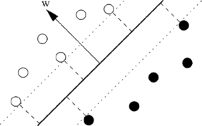
Support vector machines function by creating a hyperplane that separates a set of data containing two classes. According to the SRM principle, there will be just one optimal hyperplane, which has the maximum distance (called maximum margin) to the closest data points of each class as shown in Figure 1 (Müller et al., 2001). These points, closest to the optimal hyperplane, are called support vectors (SVs). The hyperplane is defined by the equation w·x + b = 0, and therefore the maximal margin can be found by minimizing in the following equation:

FIGURE 1 Optimal hyperplane and maximum margin for a two class data.

The optimal separating hyperplane can thus be found by minimizing Equation (1) under the constraint in Equation (2) where the training data are separated by a margin 2/‖w‖ (Burges, 1998).

The concept of the optimal separating hyperplane can be generalized for the nonseparable case by introducing a cost for violating the separation constraints Equation (2). This can be done by introducing positive slack variables ξ _i in constraints Equation (2), which then become

If an error occurs, the corresponding ξi must exceed unity, so Σ _i ξ _i is an upper bound for the number of classification errors. Hence, a logical way to assign an extra cost for errors is to change the objective function Equation (1) to be minimized into

C is a tuning parameter that allows the user to control the trade-off between maximizing the margin (first term in the objective) and classifying the training set without error. Minimizing Equation (4) under constraint in Equation (3) gives the generalized optimal separating hyperplane. This is a quadratic programming (QP) problem that can be solved here using the method of Lagrange multipliers (Haykin, 1999).

After performing the required calculations (Vapnik, 1999; Burges, 1998), the QP problem can be solved by finding the Lagrange multipliers, α _i , which maximizes the objective function in the following equation:

subject to the constraints in the following equation:

The new objective function is in terms of the Lagrange multipliers, α _i only. It is known as the dual problem: if we know w, we know all α _i ; if we know all α _i , we know w. Many of the α _i are zero and so w is a linear combination of a small number of data points. x _i with nonzero α _i are called the SVs (Gunn, 1998). The decision boundary is determined only by the SV. Let t _j (j = 1,…, s) be the indices of the s support vectors. We can write in the following equation:

Since the input vectors enter the dual only in the form of dot products, the algorithm can be generalized to a nonlinear classification by mapping the input data into a high-dimensional feature space via an a priori chosen nonlinear mapping function Φ as shown in Figure 2. Constructing a separating hyperplane in this feature space leads to a nonlinear decision boundary in the input space. An expensive calculation of dot products in a high-dimensional space can be avoided by introducing a kernel function, K in the following equation:

By introducing the kernel function, it is not necessary to explicitly know Φ(·). The optimization problem in Equations (5)–(6) can now be translated directly to the more general kernel version in Equation (9),

Kernel function, K(x _i , x _j ), plays an important role. In practice, various kernel functions can be used, such as

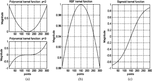
	Polynomial: K(x, z) = (〈x·z〉 +1) p
	Radial basis function:
	Sigmoid function: K(x, z) = tanh(v 〈x·z〉 +c).

The kernel function reflects the geometric relationship between the input vector and the support vector, or the similarities of the features of the faults. For example, the polynomial kernel function in Figure 3(a) describes the similarity of the two vectors, since the dot product depicts the canonical correlation. Choosing different order, p, would result in different similarity measures and hence different results. The RBF kernel function, as shown in Figure 3(b), approximates the relationship between the two vectors using a bell shaped function. Tuning the parameter s would be similar to tuning the covariance. The sigmoid kernel function in Figure 3(c) is similar to the polynomial kernel function. The parameters v and c can be used to adjust the shape of the sigmoid function (Ming, Du, Zhang, and Xu, 2004).

FIGURE 2 Mapping onto higher dimensional feature space.

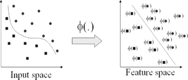
FIGURE 3 The kernel functions: (a) polynomial function with p = 2 and 3; (b) RBF function; and (c) sigmoid function.

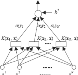
After the α _i variables are calculated, the equation of the hyperplane, d(x) is determined by the following equation:

The equation for the indicator function, used to classify new data (from sensors), is given in Equation (11) where the new data z is classified as class 1 if i > 0, and as class 2 if i < 0 (Kecman, 2004):

Note that the summation is not actually performed over all training data but rather over the support vectors, because only for them do the Lagrange multipliers differ from zero. Figure 4 illustrates the SVM data flow, from input data point to the final decision value (Ming et al., 2004).

FIGURE 4 Diagram of SVM data flow.

As such, using the SVM we will have good generalization and this will enable an efficient and accurate classification of the sensor signals. It is this excellent generalization that we look for when analyzing sensor signals due to the small samples of actual defect data obtainable from field studies. In this work, we simulate the abnormal condition and therefore introduce an artificial condition not found in real life applications.

Discrete Wavelet Transform

The wavelet transform provides a time-frequency representation of the signal. Wavelet transform uses multi-resolution technique by which different frequencies are analyzed with different resolutions. A wave is an oscillating function of time or space and is periodic. In contrast, wavelets are localized waves. They have their energy concentrated in time or space and are suited to analysis of transient signals. While a fourier transform uses waves to analyze signals, the wavelet transform uses wavelets of finite energy.

The continuous wavelet transform (CWT) is provided by Equation (12), where x(t) is the signal to be analyzed and ψ(t) is the mother wavelet or the basis function. All the wavelet functions used in the transformation are derived from the mother wavelet through translation (shifting) and scaling (dilation or compression) (Mallat, 1999).

The translation parameter τ relates to the location of the wavelet function as it is shifted through the signal. Thus, it corresponds to the time information in the wavelet transform. The scale parameter s is defined as |1/frequency| and corresponds to frequency information. Scaling either dilates (expands) or compresses a signal. Large scales (low frequencies) dilate the signal and provide detailed information hidden in the signal, while small scales (high frequencies) compress the signal and provide global information about the signal. The wavelet transform merely performs the convolution operation of the signal and the basis function. Many wavelet functions can be used and the choice of the appropriate wavelet depends on the characteristic of the signal. Examples of wavelets are the Haar and Daubechies wavelets shown in Figure 5.

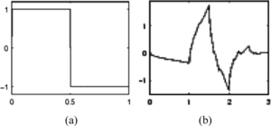
FIGURE 5 (a) Haar and (b) Daubechies 4 wavelets.

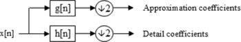
In CWT, the signals are analyzed using a set of basis functions, which relate to each other by simple scaling and translation. In the case of DWT, a time-scale representation of the digital signal is obtained using digital filtering techniques. The signal to be analyzed is passed through filters with different cutoff frequencies at different scales.

First the samples are passed through a low pass filter with impulse response g, resulting in a convolution of the two (see Figure 6). The signal is also decomposed simultaneously using a high-pass filter h:

The outputs give the detail coefficients (from the high-pass filter) and approximation coefficients (from the low-pass). It is important that the two filters are related to each other and that they are known as a quadrature mirror filter. However, since half the frequencies of the signal have now been removed, half the samples can be discarded according to Nyquist's rule. The filter outputs are then downsampled by a factor of 2. This decomposition has halved the time resolution since only half of each filter output characterizes the signal. However, each output has half the frequency band of the input, so the frequency resolution has been doubled. The coefficients are used as inputs to the SVM (Lee and Estivill-Castro, 2003).

FIGURE 6 DWT filter decomposition.

Corrosion Measurement

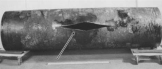
One of the biggest accidents that occurred due to pipeline failure and leakage was in Winchester, Kentucky, U.S. in 2000. It caused the pipeline owner, Marathon Ashland Pipe Line LLC a clean-up cost of around US$7 million. The crack, shown in Figure 7, was caused by a small dent in the pipe that might have been due to stone particles, coupled with the fluctuating pressures on the pipe wall which caused the pipe to fail (NTSB, 2001).

FIGURE 7 The rapture pipe due to fatigue cracking.

Wall thinning is a common occurrence in the oil piping industry; the effect of metal loss is due to high temperature, high pressure, and high flowing velocity eroding and wearing off the surface of the wall (Takahashi, Andoa, Hisatsune, and Hasegawa, 2006). The internal wall thinning of a pipe cannot be observed from the outside of the pipe; hence a method of condition monitoring using ultrasonic waves as a nondestructive test of the metal loss can help to determine when the pipe may be at risk of leaking.

The pipe with nonuniform wall thickness is subjected to combined loading by internal pressure, bending moment, and longitudinal forces. The wall thinning due to metal loss can be determined by electromagnetic or acoustic resonance such as ultrasonic and compare with a perfect pipe or theoretical pipe model. The sensors were chosen since ultrasonic sensors enable detection without any contact with the object. They are widely used in industrial application for detecting the position of the machine parts, the flow of an object on the conveyer belt, and the level of measure liquid (Lee and Estivill-Castro, 2003).

When the ultrasound propagates through the material, it creates a localized pressure change. When the pressure in the pipe raises, the molecules of the steel pipe that transmit the sound wave are packed closer; hence, the wave travels faster when the pipe is at high pressure and slower while the pipe is at lower pressure. These properties of ultrasound can be used to detect wall thinning by means of pressure change at different wall thicknesses. Ultrasonic transducers are very accurate transducers that can produce high frequency sound waves base on the piezoelectric effect (Tua, Quek, and Wang, 2005). Piezoelectric transducers have a solid-state, pressure-sensitive element that will expand and contract in step with an input voltage which is applied across the opposite terminals of the quartz crystals.

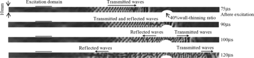
Demma et al. (2004) examined the effect of the defect size using a guided wave mode and the change of frequency of the reflection from notches. With this, they were able to show the relation between the value of the reflection coefficient and the defect size. The cylindrical ultrasonic waves provide a fast screening technique using waves that propagate along the pipe which are partially reflected when met with defects. Similar results and observations are recorded by Lin et al. (2006) using guided waves and electromagnetic acoustic transducers (EMATs) to measure wall thickness precisely. Here wave propagation experiments were performed for a specimen with a thickness of 10 mm, where different artificial defects are introduced to model local wall thinning. As shown in Figure 8, when transmitted waves impinge the wall, they are reflected and the intensity of the reflected waves vary according to wall thickness.

FIGURE 8 The energy carried by the transmitted waves pass through the wall thinning and some reflected backs as echoes.

It is therefore a well known phenomenon, both theoretically and experimentally, that defects in pipes can be detected by ultrasonic transducers (Tua et al., 2005). Having the relationship between wall thinning and a sensor signal established in prior art, our aim now is to monitor the sensor signals and use the SVM to predict the presence of defects.

METHODOLOGY

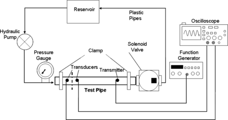
This section details the experimental set-up that will be used to simulate pipeline conditions and also defect conditions. The aim is to create a scaled-downed version of an actual section of pipeline in the laboratory using commonly available materials. Figure 9 shows the experimental set-up. A pump is used to pump hydraulic oil in the reservoir through the pipeline section. The flow rate archived is around 5 m³. A 1 m section of pipe, an outer diameter of 48.30 mm, and an inner diameter of 42 mm is connected in-between the centrifugal pump and the valve. The following are the properties of galvanized steel pipe; Young's Modulus, E (GPa): 190–210/density, ρ (kg/m³): 7850/yield strength (MPa): 340–1000.

FIGURE 9 Pipeline experimental set-up.

In order to simulate the progressive corrosion seen in real pipelines, a simulation was carried out to corrode the interior of the test pipe. In order to perform this, the test pipe is removed from the set-up. Stones and rocks of different sizes are passed through the pipe for 5 hours a day to speed up the corrosion process. This is done by recycling stones and rocks by using a conveyor belt and clamping the pipe vertically. This process is repeated daily in order to cause random metal loss in the interior of the pipe.

An ultrasonic transmitter is used to transmit a signal across the pipe and through the defect area to see changes in the ultrasound signal. The ultrasonic sensor used is the Murata analogue ultrasonic transmitter (Murata Manufacturing Company, Ltd., Japan), which is an open structure-type of sensor which has a range of up to 6 m and will be attached to the outer surface of the pipe using epoxy. MA40B8S have the nominal frequency of 40 kHz with the maximum input voltage of 40 V peak-to-peak. The stationary sensors can avoid any disturbance from the environment and will be able to transmit ultrasound along the length of the pipe by ringing the surface of galvanized steel pipe. Ultrasonic receivers, placed at the other end of the pipe, will be able to pick up the waveform that is vibrating in the pipe and can be used to monitor the condition of the pipe. The changes in the ultrasound signal will be used to determine the presence of any defects.

RESULTS

The results from the experimental rig will ultimately be used to ascertain whether SVM can detect the presence of cracks and whether DWT helps in the decision-making. Discrete wavelet transform is performed on raw time domain samples and the coefficients of the resulting DWT are input into the SVM for classification. Various wavelets can be tested including the Haar and Daubechies wavelets. A popular SVM algorithm called the Library for Support Vector Machines (LIBSVM) (Chang and Lin, 2001) is used to perform the SVM calculation. The LIBSVM includes for kernel functions: linear, polynomial, radial basis function (RBF), and sigmoid. To train an SVM, the user must select the proper C value as well as any required kernel parameters.

Time-domain samples before and after the defect area are first broken down into frames where the number of samples within the frame is a variable. Each frame will represent one instance or sample needed for the SVM and the frame size is the number of attributes or dimensions. Table 1 shows the results of the SVM accuracy in percentage as frame sizes of 50 and 25 of the same datasets are input into the LIBSVM algorithm. Ten thousand data points before the defect and 10,000 data points after the defect are used to obtain the results.

TABLE 1 Classification Accuracy (%) for Pipeline Data Using LIBSVM for Various Kernel Functions

		Frame size
Wavelet	Kernel function	25	50
–	Poly	73.68	67.74
	RBF	75.44	70.97
	Sig	73.68	67.74
DB2	Poly	83.87	61.11
	RBF	80.64	72.22
	Sig	80.64	61.11
Haar	Poly	89.65	75.00
	RBF	89.65	75.00
	Sig	86.21	75.00

As can be seen from Table 1, the smaller frame size provides better classification accuracy than the larger frame size. The RBF kernel shows the highest classification rates among the kernel functions tested. Table 2 shows the results of performing DWT on the data samples before input into LIBSVM for a period of 5 weeks. The Daubechies and Haar wavelets were used in separate instances and the results are shown.

TABLE 2 Classification Accuracy (%) Using DWT with LIBSVM for Two Different Wavelets

	SVM classification accuracy (%)
Week	Haar wavelet	DB2 wavelet	Pipe condition
Initial	89.7	80.6	Normal
1	80.4	72.2
2	75.5	66.5
3	65.5	60.1
4	50.7	54.7
5	43.9	45.6	Defect

As can be seen from the data in Table 2, the use of DWT increases the classification accuracy significantly. The classification accuracy decreases week after week showing that the condition of the pipe differs from the initial pipe condition and hence it is defective. The highest accuracy is achieved at 89.65% using the Haar wavelet with a frame size of 25.

CONCLUSION

Monitoring hundreds of kilometers of pipeline is a difficult task due to the high number of unpredictable variables involved. Rapidly changing weather conditions, pressure changes, and erosion due to gas or oil flow and ground movement are a few variables that can have direct impact on the pipeline. These variables can cause defects like corrosion, dents, and cracks which will lead to loss of the valuable commodity in addition to the serious effects on the surrounding environment.

The use of an array of sensors with help of SVM processing intends to solve these problems in two ways. Firstly, the array of sensors provides a continuous monitoring platform along the entire distance of the pipeline. Secondly, the use of artificial intelligence tools like SVM, makes it possible to monitor and ultimately predict the occurrence of defects. Support vector machines are ideal for applications like these where there are a high number of dimensions of data (sensors) and also the small number of samples for defect scenarios. Support vector machines have been used widely in many such applications and have provided an excellent generalization performance.

An experimental miniature pipeline rig provided the setting to examine the initial performance of the SVM on pipeline-like data. For now, no correlation study is made between the simulated and real situation. Acoustic sensors were used and the corrosion defect was simulated using human manipulation. The results showed good performance by the SVM using an RBF kernel function. Results with other kernels indicate that these other kernels do not accurately represent the inner product of feature vectors of that dataset. The use of DWT further improved the performance of the SVM accuracy to 89.65%. This is due to the DWT compressing the data and filtering away unwanted noise from the high frequency acoustic signals.

The conclusion is that a combination DWT and SVM algorithm can predict to a high accuracy the presence of defects in small pipes. This report will be used as a benchmark for testing on a higher scale pipeline rig, with more defect scenarios and a higher number of sensors. The ultimate aim of the research will be to predict defects before they occur thereby conserving the precious commodity and environment.

REFERENCES

- Bickerstaff , R. , M. Vaughn , G. Stoker , M. Hassard , and M. Garrett . 2002 . Review of sensor technologies for in-line inspection of natural gas pipelines, Report, Sandia National Laboratories, Albuquerque, New Mexico, USA.
- Burges , C. J. C. 1998 . A Tutorial on Support Vector Machines for Pattern Recognition . Bell Laboratories, Lucent Technologies. Data Mining and Knowledge Discovery. Netherlands .
- Chang , C. and C. Lin . 2001 . LIBSVM: A Library for Support Vector Machines. Software available at: http://www.csie.ntu.edu.tw/~cjlin/libsvm/. 20 January 2009 .
- Demma , A. , P. Cawley , M. Low , A. G. Roosenbrand , and B. Pavlakovic . 2004 . The reflection of guided waves from notches in pipes . NDT&E International 37 : 167 – 180 .
- Gunn , S. 1998 . Support Vector Machines for Classification and Regression . Information : Signals, Images, Systems (ISIS) Research Group, University of Southampton . http://www.ecs.soton.ac.uk/~srg/publications/pdf/SVM.pdf. 15 March 2009 .
- Haykin , S. 1999 . Neural Networks. A Comprehensive Foundation, , 2nd ed. , NJ , USA : Prentice Hall .
- Kecman , V. 2004 . Support Vector Machines Basics . School of Engineering Report 616, The University of Auckland http://genome.tugraz.at/MedicalInformatics2/Intro_to_SVM_Report_616_V_Kecman.pdf. 15 December 2008 .
- Lebsack , S. 2002 . Non-invasive inspection method for unpiggable pipeline sections . Pipeline & Gas Journal 59 : 58 – 64 .
- Lee , K. and V. Estivill-Castro . 2003 . Classification of ultrasonic shaft inspection data using discrete wavelet transform . In: Proceedings of the Third IASTED International Conferences on Artificial Intelligence and Application , pp. 673 – 678 . ACTA Press , Canada .
- Lin , S. , H. Fukutomi , S. Higuchi , T. Ogata . 2006 . Development of measuring method of pipe wall thinning using advanced ultrasonic techniques. Central Research Institute of Electric Power Industry (CRIEPI), Report (Q05006), Japan .
- Mallat , S. 1999 . A Wavelet Tour of Signal Processing . Philadelphia : Elsevier .
- Ming , G. , R. Du , G. Zhang , and Y. Xu . 2004 . Fault diagnosis using support vector machine with an application in sheet metal stamping operations . Mechanical Systems and Signal Processing 18 : 143 – 159 .
- Müller , K. , S. Mika , G. Rätsch , K. Tsuda , and B. Schölkopf . 2001 . An introduction to kernel-based learning algorithms . IEEE Transactions on Neural Networks 12 ( 2 ): 181 .
- National Transportation Safety Board (NTSB) . 2001 . Pipeline Accident Brief, 20594, Washington, DC. www.ntsb.gov/publictn/2001/PAB0102.pdf. 30 January 2009 .
- Shleenkov , S. , O. A. Bulychev , N. P. Nadymov , and A. B. Rogov . 2002 . Computerise magnetic testing of oil pipes . Russian Journal of Non-Destructive Testing 38 ( 6 ): 407 – 411 .
- Takahashi , K. , K. Andoa , M. Hisatsune , and K. Hasegawa . 2006 . Failure behavior of carbon steel pipe with local wall thinning near orifice . Nuclear Engineering and Design 237 : 335 – 341 .
- Tua , P. S. , S. T. Quek , and Q. Wang . 2005 . Detection of cracks in cylindrical pipes and plates using piezo-actuated lamb waves . Smart Mater. Struct. 14 : 1325 – 1342 .
- Vapnik , V. 1999 . The Nature of Statistical Learning Theory. , 2nd ed. , New York : Springer .