PREDICTING LEATHER HANDLE LIKE AN EXPERT BY ARTIFICIAL NEURAL NETWORKS

Abstract

This study developed an artificial neural network model to predict the subjective assessment of leather handle by an expert using its measurable physical characteristics. A statistical method was applied to prune the inputs of the network and the “error band” conception was proposed during training.

INTRODUCTION

Leather is a widely used material in manufacturing and its quality strongly relates to the feel of leather when handled. This is still done by experienced people such as buyers or dealers. The problem here is that manual assessment is subjective and could be imprecise and unreliable, hence objective measurement methods were developed to improve the reliability of the leather handle judgment. The BLC softness gauge (Alexander and Stosic 1993) has the potential for measuring useful physical parameters. However, the BLC softness gauge gives only one measurement of a piece of leather, while in practice a leather assessor would grade different leathers for different applications. For example, soft leather would be perfect for gloves but flimsy for shoes. Therefore, Su et al. (1996) and Huang et al. (2007) used artificial neural networks to connect the objective and subjective measurement of leather handle. Both models proved that a neural network is capable of modeling the relationships between the multiple parameters, which defines the physical properties of leather, and the subjective assessment. However, all studies until now related to manual assessment have been focused on one aspect, such as the softness of leather (Wang and Attenburrow 1994; Yu 1999), or a subjective rank by number 1 2 3 … (Su et al. 1996; Huang et al. 2007).

This study looks at the most commonly used physical measurements and mechanical properties, which relate to leather handle, as well as using a Descriptive Sensory Analysis approach to establish a comprehensive profile of leather handle. Six attributes—stiff, empty, smooth, firm, high density, and elastic, that describe leather handle from a different, more thorough, aspect were identified and quantified. Furthermore, a new pruning method called “double-threshold” was developed and worked on the network input to trim sixteen physical measurement parameters down to three—the reading from BLC gauge, the secant modulus in compression and the leather thickness measured under 1 gram load. The “double-threshold” was set to a certain significance level and used to identify the irrelevant input elements to the network model by checking if the Bayesian probability interval which was constructed by the overall connection weight of an input element to an output element, contained 0 within the constraint of two thresholds.

LEATHER HANDLE MEASUREMENT

Sample

Two collections of high quality leather were tested. The TFL collection (TFL 2006) contained thirteen pieces of bovine leather and gave quite a diversity of handling, while the PITTARDS Collection (Pittards 2007) contained nine pieces of glove leather, which were generally softer and smoother. The Artificial Neural Network used the TFL leather for training and the PITTARDS leather for testing.

Physical Measurement

Sixteen physical parameters were used as the inputs to the network. These physical parameters and the physical measurements from which they were drawn are listed in Table 1.

TABLE 1 Network Input Elements with Parameter Name, Drawn from which Physical Measurement and Short Forms

Input element	Parameter	By measurement	Short form
x1	Compressibility	Compressibility SLP52 (SLTC 2003)	com_bility
x2	Mass	Apparent density SLP5 (SLTC 1996)	mass
x3	Bending length	Drooping angel (Conabere 1941a,b,c)	bend_c
x4	Energy ratio	Vertical loop (Alexander and Stosic 1993)	loop_er
x5	Thickness	Official method SLP4 (SLTC 1996)	t0
x6	BLC softness gauge	Leather softness SLP37 (SLTC 1996)	blc
x7	Thickness (under 2 g load)	Compressibility	t2
x8	Energy ratio	Tensile strength SLP6 (SLTC 1996)	ten_er
x9	Secant modulus	Compressibility	com_mod
x10	Thickness (under 1 g load)	Compressibility	t1
x11	Apparent density	Apparent density	density
x12	Static friction coefficient	Surface friction SLP51 (SLTC 2003)	sta_c
x13	Dynamic friction coefficient	Surface friction	dyn_c
x14	Secant modulus	Tensile strength	ten_mod
x15	Energy ratio	Compressibility	com_er
x16	Linear distance	Surface friction	linear_d

Sensory Measurement

Descriptive Sensory Analysis is a technique used to obtain objective descriptions of the sensory properties of products or materials (Carpenter 2000). Seven people with much experience of handling leather were selected to work as an expert panel for assessing the leather samples after being trained so that they all agreed on the use of language and procedures. Six attributes were selected by the panel to describe the handle properties of leather and the mean value of the grades were taken as the output to the network. Table 2 indicates the panel's agreement or disagreement on the grading of each attribute over all the thirteen TFL samples by standard deviation.

TABLE 2 The Standard Deviation of TFL Leather by Attribute

Attribute	Stiff	Empty	Smooth	Firm	High density	Elastic
Std deviation	0.79	0.71	0.70	0.64	0.85	0.74

Principal Component Analysis (PCA) was applied to the panel assessment data to reduce the dimensionality of a data set (Joliffe 2002) by grouping data containing similar information (the principal component) together. This way the six attributes were grouped into three groups and it showed that stiff, empty, and smooth were the ones that were explained the most by the principal component in each group. In addition, all the panelists agreed that these three attributes were the most representative properties when assessing a piece of leather.

NETWORK MODEL DEVELOPMENT

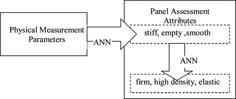
A network physical2panel was built to predict the panel assessment data from the physical measurement data. Based on those predicted data, a network panel2panel was developed to extend the prediction, which made all six attributes predictable. Thus, as illustrated by Figure 1, all six panel assessment attributes were predicted by physical measurement parameters.

FIGURE 1 Illustration of prediction from physical measurement data to panel assessment data.

As all the parameters were positive and could be easily scaled on a 0 to 1 range, the transfer function was set with LOGSIG. To avoid overtraining, ten of the TFL samples were used as training data, and the other three as validation data.

Model Panel2panel

Model panel2panel was a feed forward 3:3:3 network trained successfully with input [stiff, empty, smooth] and output [firm, high density, elastic]. The input characteristics [stiff, empty, smooth] were shown by this model to be representative of the panel assessment data.

Model Physical2panel

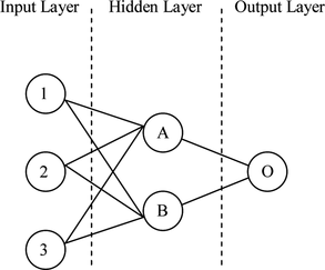
The model physical2panel was built to predict the three subjective descriptions [stiff, empty, smooth] from physical measurements. So, the next stage was to prune the input which contained sixteen physical parameters (as shown in Table 1). Different methods were considered and a statistical input pruning method proposed by Kingston et al. (2004) was selected. The method uses an overall connection weight measure to quantify the input element's relevance to the model, using a Bayesian framework to estimate the distributions of the network weights. In 2002, Olden and Jackson (2002) introduced a method of statistically assessing the importance of an input based on the comparison of the input's overall connection weight (OCW) with a statistical measure of irrelevance. The overall connection weight of an input was the sum of the products of the weights between an input and the output. An input element was considered irrelevant to the output if the OCW was equal to 0. As illustrated in Figure 2, the OCW ₁ is the contribution of input element 1 on output O. It is the sum of C _A,1 and C _B,1 which are the contributions of input element 1 via the hidden neurons A and B respectively, on the output O, as expressed by Equations (1)–(3).

FIGURE 2 Illustration of OCW with one hidden layer.

In Kingston's research, OCW was employed to quantify the relevance of the input to a model, and Bayesian probability intervals was formed to test the hypothesis that an input was irrelevant to the model. It was considered that an input was relevant to the output if its OCW was not statistically similar to zero at a high significance level (e.g., 95%). This was implemented by testing if zero lay within the interval. However, in the initial stages even important inputs might have zeros in their OCW distributions because of noise from irrelevant inputs. To ensure that important inputs were not wrongly pruned during these stages, the inputs were pruned only if their OCWs were statistically similar to zero. As the process carried on, the relationship between input and output were better defined and the variance of OCW would be less. So an important input would be less likely to contain zeros as more irrelevant inputs are pruned. Therefore, the significant level at which inputs were tested for their similarity to zero might be gradually reduced. If no OCW of input element was statistically similar to zero at 95% significance level, a 5% decrease in significance level (which was 90%) would be set to test the irrelevance until all the remaining inputs were statistically similar to zero at significance level 5%. In other words, the OCW of the inputs were not statistically similar to zero at 95% significance level.

Kingston's research was built on a network model with a single output element. However, in this study there were three output elements, stiff, empty, and smooth, so there is no direct method in Kingston's work for this situation. This made it difficult to calculate an input's importance for the whole model. For this reason, an adjustment was made when Kingston's method was adopted. Each input had an OCW on the output stiff, empty, and smooth, respectively. An input might contribute little, even zero, to one output element but greatly to another. In order to keep important input elements in the model, a “double-threshold” testing method on significance level was introduced. Significance levels at which an input was statistically similar to zero on an output were calculated. In the first stages, if an input element was irrelevant to one output element at significance level 95% (first threshold) and to the other two at higher than 75% significant level (second threshold), it was considered that this input was irrelevant to the model and could be pruned. By lowering the threshold and repeating the process, more and more input elements would be pruned. While the second threshold was always declining, the first threshold could be any value larger than second threshold. As an input might not always be very important to a particular output, it might contribute to all the three outputs at a quite important level. This means that the final conditions of Kingston's pruning method where “all the remaining inputs were statistically similar to zero at significance level 5%” (2004), might not be the final conditions in this study. It was considered that an input was important to the model if it had more than a half chance statistically similarity to zero to all the output. The pruning could be concluded by the following three steps:

1. The network model was trained 1000 times to sample the network weights and the OCW of each input element on each output was calculated. Thus an empirical distribution of the OCWs was formed.

2. Identify the irrelevant input elements by constructing the probability intervals of OCW for input element.

   • 2.1 Work out the mode of the associate weights of each input element on each output element.

   • 2.2 At first set the first threshold significance level 95% and second be 75%.

   • 2.3 If an input was at significance level 95% statistically similar to zero to one output, then this input was considered irrelevant to this particular output. Work out at which significant levels this input was statistically similar to zero to other two outputs. If both are no less than 75%, the input would be pruned from the model. Otherwise, reduce the second threshold by 5%, in this case it would be 70%, and test if the input was statistically similar to zero at this level to the other two inputs. Prune it if it was and bring the remaining inputs to the next run by going back to step 1; otherwise keep reducing the second threshold to 50% by 5% step until it found the input was statistically similar to zero at a certain significance level.

   • 2.4 If no input could be pruned by implementing 2.3, the first threshold would be decreased by 5% and step 2.3 repeated. The first threshold would not be less than the second threshold.

3. The above steps were repeated until all the remaining inputs were not statistically equal to zero for all the three outputs at a significance level of 55%, which meant the remaining inputs were all important to the model.

The process starts with sixteen-element input, and on every run of the work flow, several inputs were removed and a new model was built with fewer inputs. Table 3 shows the process of pruning the network inputs. For example there were 16 inputs of the network model at first; however, after analyzing 1000 sampled associated weights, x₂, x₇, x₁₂, and x₁₃ were considered irrelevant to the model because they were statistically similar to zero to one of the outputs at 95% significance level and 75% to the others.

TABLE 3 Process of Pruning of Inputs of Network Models

		Threshold (significant level)
Run no.	No. of Inputs	First	Second	Irrelevant inputs
1	16	95%	75%	x2, x7, x12, x13
2	12	95%	75%	x8
3	11	90%	70%	x1
4	10	95%	70%	x16
5	9	85%	70%	x11
6	8	80%	65%	x5, x14
7	6	80%	55%	x3
8	5	70%	55%	x4 x15
9	3	50%	50%	None (x6 x9 x10 remained)

Thus, a 3:4:3 model physical2panel was established, with physical parameters [blc, com_mod, t₁] on the input layer and panel attributes [stiff, empty, smooth] on the output layer.

RESULTS AND DISCUSSIONS

The generalization ability of network models was tested using data from the PITTARDS leather which had never been seen before by those models and with less discrimination in handle than TFL leather.

Results

In order to judge if the network's prediction is as accurate as the panel's assessment, a term ‘error band’ is introduced. A predication is considered successful if the difference between the desired output and network actual output is less than the panel's variance which is indicated by the squared standard deviation (as shown in Table 2). The outputs of network models were all scaled on a range from 0 to 1 for training purpose, thus need to be reverted to a range from 1 to 5 to compare with the actual grading given by panel. The desired output is the mean value of panel assessment results. If a difference is less than the standard deviation of the panel attribute, the prediction error is in an error band, which means that the prediction is successful.

The prediction results of model physical2panel are expressed in Table 4, in which all the three attributes stiff, empty, and smooth, and the sum squared error (SSE) of each sample are presented. Notice that while the SSEs are the network parameter output based on the scaled attributes on range 0 to 1, the other items in the table are unscaled values based on range 1 to 5. For each of the predicted attributes there are three columns: the first column is the output of the network, which is the prediction of that attribute; the second column, named error in the table, is the difference between the prediction and the actual panel assessment; the third column indicates whether the prediction is successful, “Y” means yes and “N” means no. The last row of the table is the mean of the absolute value of an error column or the SSE column, which is used to compare with the standard deviation of panel assessment. The last column of the table contains the SSE for each sample taking into account all the three attributes, which indicates the success of a prediction to a sample. The highest SSE of the nine PITTARDS sample is 0.41 and the lowest one is 0.01. It is shown in the table that for PITTARDS leather model physical2panel could predict 21 out of 27 attributes, or 7 out of 9 samples as accurately as the panel if taking full account of the three attributes.

TABLE 4 Prediction Results of [Stiff, Empty, Smooth] of PITTARDS Leather by Model Physical2panel

	Stiff			Empty			Smooth
Sample	Prediction	Error	Successful	Prediction	Error	Successful	Prediction	Error	Successful	SSE
01	1.07	−0.01	Y	2.41	0.41	Y	4.47	0.50	Y	0.02
02	1.15	−0.74	Y	2.31	−0.33	Y	4.50	1.71	N	0.14
03	3.13	0.37	Y	3.51	0.27	Y	4.77	0.80	N	0.03
04	1.34	−0.61	Y	2.12	−0.60	Y	4.55	3.08	N	0.41
05	1.00	−1.00	N	2.52	−0.62	Y	4.43	1.33	N	0.13
06	1.12	0.03	Y	2.35	0.41	Y	4.48	1.00	N	0.05
07	1.09	−0.70	Y	2.39	0.16	Y	4.47	−0.03	Y	0.02
08	1.05	−0.39	Y	2.44	0.44	Y	4.46	−0.12	Y	0.01
09	1.02	−0.58	Y	2.47	0.14	Y	4.45	−0.15	Y	0.02
Abs mean		0.49	Y		0.38	Y		0.97	N	0.09

While Table 4 shows numeric information of the predictions, Figure 3 gives clear pictures of the differences between the grading predicted by model physical2panel and the actual panel assessment of the PITTARDS samples by attribute. The predictions are represented by black squares, while the error bands are indicated by grey bands centred on the actual panel assessment gradings and extended up and down width 0.79, 0.71, and 0.70, respectively (the standard deviation of panel assessment on ‘stiff’, ‘empty’ and ‘smooth’). An out of band black square indicates a failed prediction, while a square in band indicates a prediction consistent with the panel grades. In Figure 3, it is clear that the panel judgements of PITTARDS leather are quite similar for stiff and empty except with sample 03; and the judgement of smooth are also alike except with sample 04. This proves what was pointed out by the panel before assessment: there are subtle differences in the glove leather data called PITTARDS.

FIGURE 3 Prediction results of [stiff, empty, smooth] of PITTARDS leather by model physical2panel (by attribute).

The prediction results of model panel2panel are expressed in Table 5, which shows predictions for firm, high density, and elastic but with the same structures as Table 4. The highest SSE of the nine PITTARDS samples is 0.09 (sample 04) and the lowest one is 0.00 (sample 06). This model predicted 22 out of 27 attributes as accurately as the panel, and fully consistent results with the panel if taking all the three attributes into account.

TABLE 5 Prediction Results of [Firm, High, Elastic] of PITTARDS Leather by Model Panel2panel

	Firm			High Density			Elastic
Sample	Prediction	Error	Successful	Prediction	Error	Successful	Prediction	Error	Successful	SSE
01	1.33	0.23	Y	2.08	0.17	Y	2.55	−0.52	Y	0.01
02	1.36	−0.27	Y	2.15	−0.64	Y	2.58	0.08	Y	0.02
03	2.43	−0.90	N	2.82	0.13	Y	2.41	0.55	Y	0.05
04	1.46	−0.65	N	2.33	−0.22	Y	2.66	−1.34	N	0.09
05	1.29	−0.72	N	2.01	−0.22	Y	2.52	−0.33	Y	0.03
06	1.35	0.17	Y	2.11	−0.21	Y	2.57	−0.22	Y	0.00
07	1.33	−0.37	Y	2.09	−0.29	Y	2.55	−0.91	N	0.04
08	1.31	0.18	Y	2.05	−0.07	Y	2.54	−0.43	Y	0.01
09	1.30	−0.18	Y	2.03	0.06	Y	2.53	−0.35	Y	0.01
Abs mean		0.41	Y		0.22	Y		0.53	Y	0.03

Figure 4 illustrates the differences between the grading predicted by model panel2panel and the actual panel assessment of the PITTARDS samples by attribute. The black squares represent predictions, and grey bands centred on the actual panel assessment gradings and extended up and down width are 0.64, 0.85, and 0.74, respectively (the standard deviation of panel assessment for ‘firm’, ‘high density’ and ‘elastic’) are indicating error bands. In Figure 4, it is clear that most of the predictions are within the error bands; the panel judgements of PITTARDS leather are quite similar on ‘high density'; and the judgement of ‘firm’ and ‘elastic’ are alike but with exception sample 03 and 04, respectively.

FIGURE 4 Prediction results of [firm, high density, elastic] of PITTARDS leather by model panel2panel (by attribute).

Discussions

Although every prediction has a difference from the desired output, only the errors noted with ‘N’ in Tables 4 and 5 need to be discussed. The error followed by ‘Y’ is in the “error band” and is less than the standard deviation of panel judgment for that attribute. This means if the network prediction is taken along with the seven panellists, the variance will be no more than that of the seven panelists. Therefore, a ‘Y’ error means that one of the panellists could have the same judgment as the network. The error with ‘N’ could be classified into two types:

1. in-range error, means that although the error is bigger than the standard deviation of the panel's judgement on the correspondent attribute, there is at least one panellist who graded the attribute with a bigger error than the prediction. This makes a prediction, even with an error noted by an ‘N’, still within the range of the seven panellist's grading. But if this type of error occurs, it might imply a low level of agreement in the panel's judgement of that attribute.

2. out-of-range error, these errors make predictions out of the range of the panel's grading for a particular attribute for a particular sample.

It is clear that the occurrence of the in-range errors might not be real errors because a panellist could make the same decision. The out-of-range error is the type of error, which needs to be discussed carefully. There are five out of range errors: four on ‘smooth’ and one on elastic. It is apparent that ‘smooth’ is the attribute that is least well predicted, while ‘empty’ and ‘high density’ are the best predicted amongst all the six attributes with no ‘N’ error at all.

The samples for which there were out-of range errors of prediction are listed, with the their distinguishable handling characteristics, as follows:

	Sample 02, which had an error, 1.71, for smooth has a pebbled surface.
	Sample 03, which had an error 0.80 on ‘smooth’ was considered having a “hard, papery, plastic surface which is grippy” by A panellist.
	Sample 04 is a piece of leather with embossed surface. A panellist confirmed that the result might be “texture affected.” It had an error 3.08 on ‘smooth’ and −1.34 on ‘elastic’.
	Sample 05, which had an error 1.33 on smooth is a piece of leather with an intended scratched surface.

In this study, the size and diversity of training samples are considered the main reason causing the prediction to differ from the actual panel assessment. The network models learn relationships between input and output from the paired data of the training samples and predict the output of the testing samples based on the relationship learnt. If there are not enough typical samples, a network will be short of information required to do the prediction task. Although the thirteen TFL samples were selected carefully to be typical and sufficient to cover as much as possible different types of leather, it was possible that some sorts of leather were missing as there are so many leathers with different handle characteristics.

In fact most the TFL samples were upholstery leather, while the testing samples, PITTARDS, are thin and soft glove leather. The PITTARDS leather samples could be considered as one type of training sample set as the handling characteristics are quite similar. This explains why the prediction trends in Figures 3 and 4 are relatively flat. But it is exciting that although the prediction trends are not always within the error bands, the distribution of the squares on the graphs still shows that the network could tell the subtle differences between the leather handle characteristics. This provides further proof that the network models found meaningful relationships between the input and the output.

CONCLUSION

Artificial neural network models were developed to predict six attributes (stiff, empty, smooth, firm, high density, and elastic) like experts from three physical parameters (BLC gauge reading, compression secant modulus and thickness). A statistical pruning process “double-threshold” was used to decide if an input was irrelevant to a network model by adjusting the significance level. In comparison between the prediction and the panel assessment attributes, “error band” was brought forward and allowed a tolerance of errors that the panel could make. The full-scale prediction of leather handle by those network models is more universal and shows how leather handle is directly perceived allowing value judgments to be made later when an application has been decided.

REFERENCES

- Alexander , K. T. W. , and R. G. Stosic . 1993 . A new non-destructive leather softness test . Journal of the Society of Leather Technologists and Chemists 77 ( 5 ): 139 – 142 .
- Carpenter , R. P. , D. H. Lyon , and T. A. Hasdell . 2000 . Guidelines for Sensory Analysis in Food Product Development and Quality Control, ed , 2nd . Gaithersburg: Aspen.
- Conabere , G. O. 1941a . Measuring the feel of leather: Part I. The use of the peirce flexometer to test the “feel” of leather . Journal of International Society of Leather Trades' Chemists 25 ( 8 ): 245 – 253 .
- Conabere , G. O. 1941b . Measuring the feel of leather: Part II. The measurement of the stiffness of chrome calf upper leather . Journal of International Society of Leather Trades' Chemists 25 ( 8 ): 298 – 305 .
- Conabere , G. O. 1941c . Measuring the feel of leather: Part IV. The measurement of the firmness and fullness of chrome calf upper leather . Journal of International Society of Leather Trades' Chemists 25 ( 10 ): 319 – 329 .
- Huang , X. , X. Zhang , and M. Wang . Evaluation of leather handle character using neural networks . Journal of the Society of Leather Technologists and Chemists 91 ( 4 ): 172 – 174 .
- Joliffe , I. T. 2002 . Principal Component Analysis, ed , 2nd . (Springer Series in Statistics). New York : Springer .
- Kingston , G. , H. R. Maier , and M. F. Lambert . 2004 . A statistical input pruning method for artificial neural networks used in environmental modeling. In The International Environmental Modelling and Software Society iEMSs 2004 International Conference. University of Osnabruck, Germany: iEMSs 2004, 2004.
- Olden , J. D. , and D. A. Jackson . 2002 . Illuminating the “black box": A randomization approach for understanding variable contributions in artificial neural networks . Ecological Modelling 154 ( 1–2 ): 135 – 150 .
- Pittards. Pittards plc. http://www.pittards.com/ (accessed October 2, 2007).
- SLTC. 1996 . SLP37 Measurement of leather softness. In the Official Methods of Analysis. The Society of Leather Technologists and Chemists.
- SLTC. 1996 . SLP4 measurement of thickness. In the Official Methods of Analysis. The Society of Leather Technologists and Chemists.
- SLTC. 1996. SLP5 Measurement of apparent density. In the Official Methods of Analysis. The Society of Leather Technologists and Chemists.
- SLTC. 2003 . SLP51 Measurement of surface friction. In the Official Methods of Analysis. The Society of Leather Technologists and Chemists.
- SLTC. 1996 . SLP52 Measurement of compressibility. Official Methods of Analysis, The Society of Leather Technologists and Chemists, 2003.
- SLTC. 1996 . SLP6 Measurement of tensile strength and percentage elongation. In the Official Methods of Analysis. The Society of Leather Technologists and Chemists.
- Su , Z. , G. Yin , and Z. Zhuo , 1996 . Objective evaluation of leather handle with artificial neural networks . Journal of the Society of Leather Technologists and Chemists 80 ( 4 ): 106 – 109 .
- TFL. TFL Academy. http://www.tfl.com/default.asp (accessed May 10, 2006).
- Wang , Y. L. , and G. E. Attenburrow . Factors influencing the softness of brazilian goatskin leathers . Journal of the Society of Leather Technologists and Chemists , 78 ( 3 ): 85 – 87 .
- Yu , W. 1999 . The mechanical properties of leather in relation to softness. Thesis, University of Leicester, Leicester, UK.