Application and Experimental Validation of Pheromone Design in Ant Colony Optimization: the Problem of Robot Skin Wiring

Abstract

During the past few years, the problem of optimally routing the wiring in large-scale modular skins for robots gained much attention in the literature. From a theoretical standpoint, the problem is NP-hard. Following previous work (Anghinolfi et al. 2012; Nattero et al. 2012), we solve the skin wiring problem using an ant colony optimization approach. In this article, we specifically address the problem of designing a pheromone structure that is effective in terms of solution quality. In particular, we propose five different alternatives, which are thoroughly validated using problem instances originating from both real and theoretical (i.e., artificially generated) use cases.

Introduction

In order to provide robots, especially humanoid robots, with tactile sensing capabilities, the development of a so-called robot skin has been an active field of research in the past few years (Dahiya et al. 2010). A robot skin is a sensing device composed of a (usually huge) number of tactile sensors linked in a network of connections. As a matter of fact, robot skins are expected to enable new means of physical interaction between humans and robots (Argall and Billard 2010). Furthermore, because a robot skin covers robot surfaces on the large scale, it usually enforces a safer and a more natural interaction.

Different transduction principles have been exploited to allow for the detection of different types of information: pressure, proximity, or temperature, as discussed by Dahiya and colleagues (2010). Independently from the employed mechanical transduction principle, to design a full-fledged robot skin is a difficult engineering task, because it requires dealing with a number of conflicting requirements in terms of resolution (Shimojo 1994), reaction dynamics and bandwidth (Baglini, Cannata, and Mastrogiovanni 2010), weight, energy consumption, optimal placement and calibration (Cannata, Denei, and Mastrogiovanni 2010c), as well as reliability and real-time software performance (Cannata, Denei, and Mastrogiovanni 2010b; Youssefi et al. 2011), to name but a few.

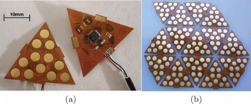
The robot skin we target in this work exploits capacitance-based transducers (Cannata et al. 2008; Cannata, Dahiya, Maggiali, et al. 2010; Schmitz et al. 2011) organized in equilateral triangular modules. There are 12 tactile elements (referred to henceforth as taxels) on each module, which is made by flexible printed circuit board (PCB) and also hosts the read-out electronics, as shown in Figure 1a. Triangular modules can be interconnected in order to cover, through appropriate algorithms (Anghinolfi et al. 2013), a large robot body part. Each triangular module can be connected to up to three other adjacent triangular modules. A set of modules covering a part of a robot is called a patch (Figure 1b). Each patch is managed by a set of external microcontrollers, responsible for the transmission of tactile sensory data to an embedded PC for further data processing, thereby implementing high-level tactile-based behaviors, such as those described, for example, Cannata, Denei, and Mastrogiovanni (2010a) and Denei, Mastrogiovanni and Cannata (2012). Each microcontroller has a capacity of up to C = 16 modules. The data network between the single triangular module read-out electronics and the patch microcontroller is embedded in the PCB. As a matter of fact, thanks to I/O ports on triangular module sides, tactile sensory data can be sent to and forwarded from adjacent modules, eventually reaching a specific I/O port of the patch connected to the external microcontroller.

FIGURE 1 (a) A skin triangular module PCB, front and rear sides; (b) a patch of interconnected modules.

In the early stages of skin design, an appropriate routing of the connections between adjacent triangular modules is necessary in order to efficiently link each triangular module to an appropriate microcontroller. It is noteworthy that the skin wiring problem represents one of the major limiting factors to the implementation of large-scale robot skin, because of the physical space (which is very limited in robots) needed to convey all the signal cables when large-scale robot surfaces must be covered. In order to reduce the wiring complexity, in the reference technology each microcontroller can be directly connected to one element of a patch only, which is referred to as the entry point, whereas the signal cables of other triangular modules are routed via neighboring modules. Then, each module can route data signals related to the taxels managed by a single microcontroller.

The skin wiring problem consists, therefore, of choosing how to route the signals from a specific triangular module to the assigned microcontroller, possibly satisfying (at the same time) different functional requirements, vis., power consumption, which is mostly related to the number of employed microcontrollers, and fault tolerance. The former is achieved by reducing the number of microcontrollers to the minimum needed to control all of the triangular modules, whereas the latter prescribes that, in case of failure, at least a graceful performance degradation of the robot skin subsystem must be achieved, because a residual functionality is essential in order to detect the failure and lead the robot safely home.

The failure of a microcontroller is considered the most critical situation, because it affects all the associated triangular modules. As a matter of fact, it can cause large parts of the sensing surface to stop working. Intuitively, as it has been shown by Anghinolfi and coauthors (2012), in order to reduce the effects of such a failure, it is advisable to (1) uniformly distribute the load among micro-controllers, and (2) spread the triangular modules assigned to a microcontroller as much as possible with respect to the robot surface that must be covered.

These concepts lead to the formulation of skin wiring as an optimization problem with three distinct but interconnected aspects (Anghinolfi et al. 2012):

1. Assign each triangular module to a microcontroller.

2. Identify an entry point in the patch for each microcontroller.

3. Define wire routing in terms of interconnections between I/O ports.

A general optimization technique based on ant colony optimization (ACO) has been discussed by Anghinolfi and colleagues (2012) and Nattero and coauthors (2012). The main contribution of this article is a computational analysis of different pheromone structures for the same ACO algorithm. This article is organized as follows. A graph theoretical problem definition is given in “Problem Statement”, followed by a review of relevant literature in “Related Work.” “Mathematical Formulation” reports a mixed integer programming (MIP) formulation for the problem. We describe a multistart heuristic and an ACO-based approach, together with five different pheromone structures in “A Solution to the Skin Wiring Problem”. In “Experimental Analysis,” we test and discuss the performance of the five heuristic approaches, and we draw conclusions in the final section.

Problem Statement

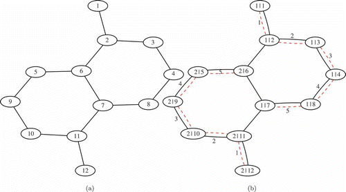
It is convenient to represent a robot skin patch using a graph , where is a set of nodes representing skin triangular modules and is a set of edges representing links between adjacent modules. An example of a graph associated with a patch is given in Figure 2a.

FIGURE 2 (a) An example of a graph representing a patch; (b) a possible solution to the associated skin wiring problem.

It is noteworthy that the graph is supposed to be symmetric. As a consequence, no direction is defined between two connected modules. Due to the characteristics of the considered robot skin and independently from the module shape, G is a planar graph. In addition, if the nodes associated with the triangular modules on the border are neglected, then G is also a regular graph. Given a patch and a corresponding graph G, D_ij represents the Euclidean distance between the centroids of each pair of triangular modules . Finally, a set of q microcontrollers is given.

The problem of optimally defining a wire routing for a patch of triangular modules can be modeled within the class of the Constrained Spanning Forest problems: the set of triangular modules assigned to a microcontroller k corresponds to a set of nodes T_k, such that (i.e., the maximum number of triangular modules that can be managed by a microcontroller), and the wiring defines an acyclic connected subgraph in G induced by T_k, in other words, a tree. Any node v in T_k can be chosen as a root and used as the entry point for the microcontroller k. The solution of the skin wiring problem is then a forest F corresponding to the collection of all the trees S_k. As a consequence, the solution satisfies the constraints because the connections of triangular modules in a patch to a set of microcontrollers and the consequent wire routing correspond to a constrained spanning forest on the graph associated with the patch. As an example, Figure 2b shows a possible wiring for the patch graph of Figure 2a using two microcontrollers. In Figure 2b, node labels (k|v) denote the microcontroller index followed by the node index, whereas the number associated with the edges represents the order of assignment of a connection to a microcontroller, thereby allowing for the identification of the entry points (nodes 1 and 12 in the example) and the routing direction.

Related Work

The Problem of Wiring in Robot-Skin Design

During the past few years, research activities on large-scale tactile technology for robots exploited wiring patterns in which the tactile elements are located on the nodes of a regular square grid (Allen and Michelman 1990; Lazzarini, Magni, and Dario 1995; Hwang, Seo, and Kim 2007; Goger and Worn 2007; Chang et al. 2007; Duchaine et al. 2009; Shimojo et al. 2010; Lacasse, Duchaine, and Gosselin 2010). This is due to the relative simplicity of such a design at the electronics and wiring levels. All the approaches proposed in the literature address the trade-off between the number of actual signal wires needed to physically transmit tactile data, the density of sensors, and the resulting complexity of ancillary electronics and cabling.

As a matter of fact, solutions based on grid-like regular patterns are not efficient when scaling up to large surfaces of robot skin including hundreds or thousands of tactile sensors, because the number of wires quadratically increases with the size of the tactile array. This issue is of the utmost importance, especially in highly embedded machines such as humanoid robots, because the physical space necessary to host wires can be often difficult to obtain. In order to overcome this problem, it is often suggested to introduce multiplexing components, which are able to provide taxel readings at the price of a lower tactile data acquisition rate. However, the introduction of additional electronic components is in contrast with the aforementioned lack of available physical space.

Wiring in large-scale robot skin has been considered under a different perspective by Jockursh, Walter, and Ritter (1997); Nilsson (1999); and Futai and colleagues (1999); in whose works smart solutions for minimizing the number of wires out of tactile surfaces have been envisaged, and which do not need any data multiplexing, but at the cost of an increased complexity in electronics (i.e., the space needed to host the electronics itself) and protocols for data acquisition (i.e., higher latency).

Two well-known examples are aimed at avoiding the problem of wiring altogether. The principle of a telemetric robot skin has been presented by Hakozaki, Oasa, and Shinoda (1999); Shinoda and Oasa (2000); and Hakozaki and Shinoda (2002). According to this approach, wireless sensor modules managing pressure and physical deformation transducers are located inside a mould material, which is drained inside a suitable robot cover. So far, apart from a proof-of-concept design and a quite-small implementation, the use of telemetric robot skin in real-world, large-scale surfaces is still to be evaluated. Furthermore, this design approach suffers from the impossibility of precisely defining where the tactile sensors are located after the entire process, which is a desirable feature in real-world robots.

A deformable and stretchable skin system is discussed by Alirezarei, Nagakubo, and Kuniyoshi (2007) and Nagakubo, Alirezarei, and Kuniyoshi (2007), wherein the principle of electrical impedance tomography is exploited to reconstruct a pressure distribution over a given surface using measurements taken only at the border of the same surface. Although this approach avoids wiring the tactile surface itself, the problem is just shifted to the number of wires actually needed to take reliable measurements at the border (especially when large-scale robot surfaces are the target).

The problem of wiring in robot skin design has been addressed in a principled way only by Hoshi and Shinoda (2006a,b), Schmitz and coauthors (2011), Mittendorferand Cheng (2011), and Anghinolfi and colleagues (2012). It is interesting to note that all of these approaches represent examples of modular skin design. Apart from minor details, these robot skin designs are made up of a number of basic sensing modules, each one hosting a number of tactile elements as well as ancillary read-out electronics. In order to build large-scale tactile surfaces, it is necessary to interconnect a (typically huge) number of basic units. Such an interconnection is also used to transmit local tactile data to a centralized processing node.

To this aim, each basic module must provide a well-defined signal routing such that, when interconnected with other modules, the overall network is consistent and efficient. The work described by Hoshi and Shinoda (2006a,b) provides a solution for a specific shape of basic modules. Although the solution proves to be efficient, the design is not characterized by any optimality principle (i.e., robustness, efficiency, fault tolerance) leading to an appropriate wiring. The same can be argued for the work presented by Schmitz and colleagues (2011), in which the wiring between modules is fixed. Self-configuration capabilities have been implemented in the Hex-O-Skin technology (Mittendorfer and Cheng 2011). However, it cannot be proved that the obtained configuration is able to enforce any optimality principle. Starting from the robot skin design introduced by Schmitz and coauthors (2011), we presented heuristic algorithms in Anghinolfi and coauthors (2012) to provide a reasoned trade-off between the need for a modular design and (to a limited extent) the requirements associated with robustness and fault tolerance. In particular, the main proposed algorithm is based on an ACO approach, which we recently improved in Nattero and colleagues (2012).

Constrained Spanning Forests

The Maximum Weight Forest (MaxWF) problem consists of defining a spanning forest that maximizes the sum of the weights associated with each edge. Although it is possible to solve MaxWF in polynomial time with a greedy algorithm (Papadimitriou and Steiglitz 1982), the introduction of constraints makes the problem much more difficult. The Maximum Weight t-restricted Forest (MaxWCF(t)) problem, consisting of finding the MaxWF constrained to have no more than t edges in each tree, has been shown to be NP-hard (Gupta et al. 2010). Furthermore, the authors give a approximating greedy algorithm. Imielinska, Kalantari, and Khachiyan (1993) deal with the Minimum Weighted Constrained Spanning Forest (MinWCF(p)) problem, which consists of computing the spanning forest of minimum weight such that every tree component contains at least p nodes. In particular, they demonstrate that the problem is NP-hard, , whereas Monnot and Toulouse (2007) show that MinWCF(p) is NP-hard even with p = 3. Bazgan, Couëtoux, and Tuza (2011) address the unweighted version of the same problem (MinCF(p)) and show that it is NP-hard for any p ≥ 4, even on planar bipartite graphs of maximum degree 3. Moreover, they demonstrate that, by dropping the condition of planarity, the problem becomes APX-hard for any p ≥ 3, even on graphs with maximum degree 3.

Despite a number of similarities, the skin wiring problem differs both from MaxWF and MinWCF (as well as from MinCF). As a matter of fact, the problem considered here is to find a constrained spanning forest F that serves all nodes, minimizing a cost function with two components:

1. The sum, for all the trees , of the absolute value of the difference between the number of nodes |T_k| and the desired average number of nodes per tree, defined as (where |K| is the number of trees), which is expected to favor the microcontroller load balancing.

2. The sum, for all the trees and for all the ordered pairs of nodes (i, j), such that , of the difference between the maximum distance between all the pairs of nodes in V and the distance between i and j, which is expected to favor the spreading of triangular modules associated with a single microcontroller.

Considering the second objective component, it is evident that, for the faced Constrained Spanning Forest problem, no cost can be a priori associated with an edge because it depends on which subsets of nodes in V are finally assigned the |K| trees. As a consequence, because the contribution of an edge to the objective function becomes known only after the introduction of that edge in a solution, a greedy heuristic appears not to be suitable for the skin wiring problem. Nonetheless, if the contribution of each edge were known a priori, the considered problem could be reduced to a MinWCF. This allows us to conclude that the problem is NP-hard.

Graph Clustering and Partitioning

During the past few decades, graph clustering represented a field of active research (Schaeffer 2007). In particular, the basic problem consists of grouping graph nodes into clusters in order to maximize the number of edges within each cluster and to minimize the number of edges between clusters. Although it can be argued that the skin wiring problem belongs to the family of graph clustering problems, typical graph clustering does not explicitly address the connectivity constraints that we face in our case (because of the adopted technology) and which makes the problem much more dificult. The work by Yan, Zhou, and Han (2005) is one of the few considering such constraints explicitly. However, the authors do not address cardinality constraints, which is a specific requirement in our case.

Graph partitioning, packing, and covering (Feder et al. 1999) consist of grouping the nodes of a graph such that each node is assigned to, respectively, exactly one, at most one, or at least one graph subset. These problems are closely related to the topic of this article. However, connectivity is not explicitly enforced in the standard formulation of the problem.

A close class of problems is the graph tree partition (GTP), in which the graph must be partitioned by means of trees. These problems are NP-hard in many relevant cases, as has been demonstrated by Cordone and Maffioli (2001). In GTP problems, connectivity is ensured by the existence of trees. However, the difference with the problem we discuss in this article resides in the objective and the cardinality constraints. It is worth noting that Cordone and Maffioli (2001) can successfully solve the problem by means of an ACO approach.

Mathematical Formulation

The skin wiring problem can be formulated as the problem of determining a spanning forest on the graph associated with a skin patch so that the forest is composed by at most |K| trees, and each tree includes at most C nodes. In addition, because for each microcontroller an entry point and a feasible routing must be determined, for each tree a root node and an orientation is selected so that the solution corresponds to a directed spanning forest consisting of a set of arborescences.

The problem can be formulated as a mixed integer programming (MIP) problem considering the directed graph , where , and . The node s is a dummy node used as a root. In the following, let denote a generic directed arc, where nodes i and j are respectively the tail and the head of a. Then, a feasible solution identifying a directed spanning forest H is a set of arborescences R_k, that is, , where and . The following constants are used:

• D_ij, , is the Euclidean distance between nodes i and j.

• .

• .

• C is the maximum number of nodes in a tree (i.e., the microcontroller capacity, which is 16 in our case).

• is the desired number of nodes in a tree (i.e., the desired microcontroller load level).

• are the weights modeling the priority of the objective function components.

The following decision variables are used:

• , ;

  if and only if controller k ∈ K is connected directly to node v ∈ V, that is, v is the root of tree k (i.e., the entry point for microcontroller k).

• , ;

  if only if ; a node j is assigned to an arborescence (i.e., it is controlled by microcontroller k) if either j is the root of k or it is the head of an arc such that .

• , , i < j; y_ij = 1 only if for a given k; these variables determine if two nodes are assigned to the same arborescence and are used to evaluate the relative distance between nodes.

• , ; n_v = 1 only if ; variables n_v are introduced to relax the node spanning condition, i.e., to model also the case of skin patches that generate graphs structured so that there is no possibility to assign all the nodes to a microcontroller (this point is discussed later in this section).

• , ; these are deviational variables giving the absolute difference between |T_k| and the average desired load λ for microcontrollers.

• , ; variables used in subtour elimination constraints.

Skin wiring is a multiobjective problem requiring the minimization of the three following objectives:

(1)

(2)

(3)

where O₁ (1) is the sum of unassigned nodes in the current solution, O₂ (2) is the sum over all microcontrollers of the variations from the average desired load λ, and O₃ (3) corresponds to the sum of the normalized distances among every pair of nodes assigned to the same arborescence.

The following three scaling factors, ν₁, ν₂ and ν₃, are introduced to ensure that , :

(4)

Note that, because such factors are derived from worst case considerations, the scaled objectives cannot reach the extremes of their variation range.

The multiobjective problem can be converted into a scalar minimization problem by combining the three objectives into a single weighted additive objective function, in which the values of the weights are provided according to the different preference of the decision maker. As a matter of fact, a lexicographic priority can be imposed between any pair of objectives O_i, O_j, fixing . Then, the proposed formulation is as follows:

(5)

subject to:

(6)

(7)

(8)

(9)

(10)

(11)

(12)

(13)

Constraints (6) require that each node is assigned, at most, to a single arborescence (i.e., a microcontroller), being either the entry point for the arborescence or the head of one of its arcs. Constraints (7) ensure that an arc with origin in node i can be assigned to controller k only if another arc assigned to k enters in i or if i is an entry point for k. Constraints (8) impose that for each microcontroller there is, at most, one entry point. Constraints (9) limit the number of nodes assigned to each microcontroller to C, taking into account the fact that a node j is assigned to a microcontroller k, or an arc exists insisting on j and starting from a node assigned to k. Constraints (10) are the subtour elimination constraints introduced by Miller, Tucker, and Zemlin (1960). These constraints ensure that each microcontroller is associated with an acyclic connected and directed subgraph, that is, an arborescence. Constraints (11) and (12) define the unbalance between the number of nodes assigned to a microcontroller k and the average desired load. Constraints (13) impose y_ij = 1 if nodes i and j are controlled by the same microcontroller, specifically by the first and the second summation. Variables n_v are necessary to determine feasible solutions for the graphs whose nodes cannot be partitioned into |K| distinct arborescences (i.e., assigned to the available |K| microcontrollers). Such situations may arise in the case of patches generating a nonconnected graph, but also in the case of a connected graph with particular structures (Anghinolfi et al. 2012).

A Solution to the Skin Wiring Problem

An ACO Algorithm for Optimal Skin Wiring

Because the MIP model as is cannot handle large-scale instances (Anghinolfi et al. 2012),a metaheuristic approach has been developed and, being that the problem instances are very structured, the choice has been oriented toward an algorithm that makes use of learning. In particular, an ACO algorithm (Dorigo and Blum 2005), together with an efficient candidate strategy (CS), has been implemented (Anghinolfi et al. 2012). The ACO algorithm described in this section shares the same structure of the algorithm introduced by Anghinolfi and Paolucci (2008), which borrows concepts both from the ant colony system (ACS); Dorigo and Gambardella 1997) and the max-min ant system (MMAS) frameworks (Stützle and Hoos 2000).

Table

Pseudocode 1. An ACO Algorithm for the Skin Wiring Problem
Input: a graph , the number of microcontrollers |K|, the desired occupancy level λ, and the number of ants P.
1:
2:zbest
3:π ← initPheromone(G)
4:while termination_condition not met do
5: for all ant a do
6:  Fa ← buildSolution(G, |K|, λ, π)
7:  if zbest then
8:
9:
10:  end if
11:  localPheromoneUpdate(Fa, π)
12: end for
13:  globalPheromoneUpdate(F*, π)
14:end while
15:return F*

The algorithm is outlined in Pseudocode 1. The algorithm requires the graph G, the number |K| of microcontrollers, the desired occupancy level λ, and the number P of artificial ants. The best solution F* and the best value z_best are initialized, respectively, to an empty set (line 1) and to +∞ (line 2). The pheromone π is also initialized at line 3. The main loop (lines 4–14) consists of making each ant construct a forest F_a that possibly spans all the nodes in V (line 6), comparing the solution against the incumbent and eventually save it (lines 8–9).

Pheromone trails are locally updated after each construction (line 11) and globally updated at the end of the iteration (line 13). The best found solution is finally returned (line 15).

As discussed by Anghinolfi and colleagues (2012), the solution construction proceeds incrementally, because each ant a constructs a forest F_a by adding one tree T at a time. A tree is constructed by adding an edge e to T. The edge e is obtained from an element z, which is extracted out of a set Θ of candidates using information associated with pheromone trails. The set Θ is generated from scratch before the insertion of each edge (refer to the following two subsections). The set Θ can contain two possible types of elements, edges or nodes. A node v is called free if it has not been assigned to any tree yet. If z corresponds to an edge , either i ∈ T and j is free, or j ∈ T and i is free. In the other case, if z corresponds to a node v, then it is free. For the sake of completeness, any edge e connecting v to a node in T can be added, because their contribution to the objective function (5) is equivalent. The construction of the current tree ends when the desired occupancy level has been reached (i.e., when |T| = λ) or when it is no longer possible to find an element for which the insertion is feasible (i.e., when ).

Note that, for comparison purposes, it is possible to design a randomized constructive heuristic simply by neglecting the use of pheromone trails. In this case, the selection of the next element z ∈ Θ to insert in T is randomly performed with a uniform probability distribution. A multistart heuristic (MSH) is then obtained by restarting the construction. Conceptually, this approach corresponds to using one ant only (i.e., to setting P = 1), but in practice, it is convenient to implement a dedicated algorithm. For a fair comparison, the termination condition of both MSH and ACO is the maximum running time.

Differently from MSH, when more alternatives exist, the ant performs the selection in two steps. First, as in the standard ACS, the ant randomly chooses the node selection rule between exploitation and exploration with probability and 1 – q, respectively. Let π(z) denote the pheromone trail associated with element z. Then, the exploitation rule selects z deterministically according to

(14)

and the exploration rule selects z according to a selection probability p(z) obtained as

(15)

Following the same approach proposed by Anghinolfi and Paolucci (2008), the pheromone trails do not depend on the cost function values associated with previously explored solutions. Rather, they vary in an arbitrary range such that and . In this way, π_min and π_max are no longer parameters to be tuned. This feature makes the algorithm independent from the specific problem or instance. After an ant a completes the construction of a solution F, in order to reduce the probability that the successive ants construct an identical solution during the same iteration, the pheromone trails are locally updated (line 11 in Pseudocode 1) as follows:

(16)

where is the local evaporation parameter. The global pheromone update (line 13) is performed in three steps:

1. Perturbations due to the local pheromone updates are removed.

2. Pheromone trails are evaporated as follows:

   (17)
   where F* is the incumbent solution and is the global evaporation parameter.

3. Pheromone trails relevant to F* are reinforced as follows:

   (18)
   where Δπ(z) is the maximum pheromone reinforcement obtained as
   (19)

As shown in Anghinolfi and Paolucci (2008), these rules make the pheromone reach both bounds asymptotically.

Definition of the Candidate Strategy

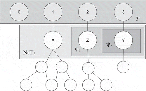
The set Θ of candidate elements for insertion is constructed, coherently with the used pheromone structure, upon a set Ψ of candidate nodes, which is defined as follows. Let A(v) be the set of nodes adjacent to v and be the set of free nodes adjacent to v. With a minor abuse in the notation, let also A(T) be the sets of nodes adjacent to those in T and N(T) the set of free nodes adjacent to those in T. Given an incomplete forest F, possibly empty, a first set Ψ₀ is obtained including all nodes in N(T). If the tree T is empty, then any free node is added to Ψ₀ to initialize its construction. It is possible to pass directly Ψ = Ψ₀ to an ant, but this choice leads to poor-quality solutions, which, most of the times, are also incomplete. A first improvement is obtained by constructing a set keeping only those nodes for which |N(v)| is minimal:

(20)

This is called the least unassigned (LU) rule and allows us to obtain much better solutions, although it still produces too many incomplete ones.

Finally, a set can be defined by keeping only those nodes in Ψ₁ for which, in turn, the total number of free adjacent nodes is minimal:

(21)

This is called the least cumulative unassigned (LCU) rule and, thanks to its look-ahead effect, it reduces the chances that a node v is left unassigned to any microcontroller because it tends to avoid leaving v isolated.

It is convenient to set : LCU allows us to obtain remarkably better solutions in terms of objective O₁, and partly of O₃ because, in most cases, this mechanism favors the generation of chain-like shaped trees (i.e., trees with only two leaves). Objective O₂ is implicitly taken into account by limiting the number of nodes per tree to λ.

Figure 3 shows how the LCU rule works. Let us assume . Then . All nodes in N(T) have only one free adjacent node, except for X. Therefore, . The cumulative sum of free adjacent nodes for Y is 1, whereas it is 3 for Z, thus .

FIGURE 3 Candidate set generation.

Pheromone Structures

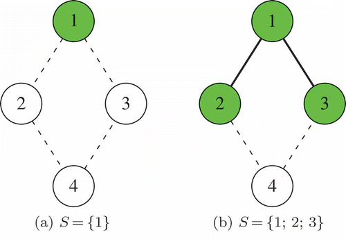
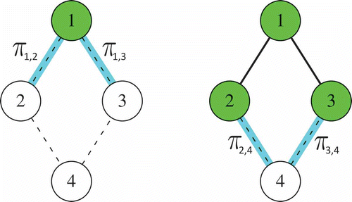
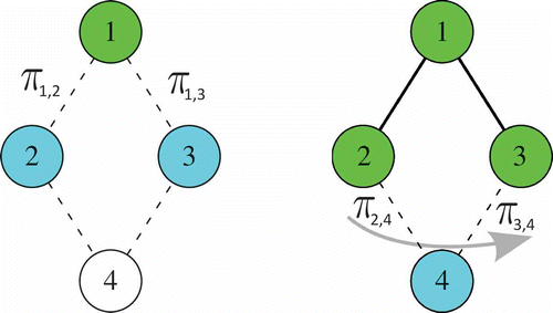
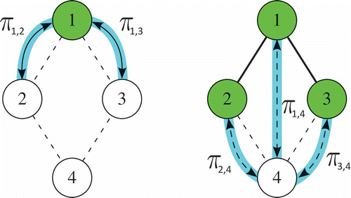
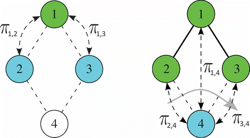
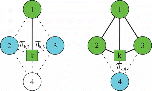
The pheromone allows the artificial ants to learn which attributes characterize good solutions. The candidate set must be coherent with the choice. To better explain the structures that we explore throughout the remainder of this section, we consider the scenario depicted in Figure 4, which represents part of a graph where a tree is under construction. Specifically, Figure 4a shows a case where only node 1 is assigned to the tree, whereas in Figure 4b nodes 2 and 3 have been added.

FIGURE 4 Two partial solutions for the same graph , where and .

Because in this problem it is necessary to learn how nodes link together, we have tested the following possibilities.

Direct Edges (DE). In this case, Θ is defined as the set of edges linking a candidate node and a node in current tree:

(22)

The pheromone trail is associated with each edge e ∈ E and is indicated as π_e. Figure 5 shows the pheromone trail and the candidates.

FIGURE 5 A direct edges structure, where (a) , and (b) , .

Cumulative Edges (CE). In this case we have:

(23)

and the value of the corresponding pheromone trail π_v is averaged over all possible edges e linking v to a node in T:

(24)

where is defined as:

(25)

This is the pheromone structure originally adopted by the authors in (Anghinolfi et al., 2012) and is shown in Figure 6.

FIGURE 6 A cumulative edges structure, where (a) , , , and (b) , , .

Direct Pairs (DP). In this case, Θ is the set of (virtual) edges linking all nodes in T with all nodes in Ψ:

(26)

where

(27)

The pheromone structure is associated with the same edges. Figure 7 shows how this structure works.

FIGURE 7 A direct pairs structure, where (a) , and (b) , .

Cumulative Pairs (CP). This structure behaves as in the CE case, but is applied to pairs defined as in the previous case:

(28)

and the pheromone trail is averaged over all edges in ending or beginning in v:

(29)

The behavior of this structure is further explained in Figure 8.

FIGURE 8 A cumulative pairs structure, where (a) , , , and (b) , .

Naive Clustering (NC). In this case, the element to be inserted is a node:

(30)

and the pheromone π_c is associated with the ordered couple c = (T, v), where T is the tree under construction and . This representation is the only one that works also with empty trees, whereas the others require the adoption of dummy edges to initialize the construction.

The naive clustering is depicted in Figure 9.

FIGURE 9 A naive clustering structure, where (a) , and (b) , .

Experimental Analysis

Generation of Problem Instances

We consider three sets of instances, which we refer to as i, s, and t. Dataset i contains real instances corresponding to patches for body parts of the iCub robotic platform,¹ and has a number of nodes ranging from 6 to 232. These instances correspond, respectively, to: i1 = left upper arm, lower part; i2 = left hip; i3 = right upper forearm; i4 = upper torso; i5 = lower torso.

Dataset s contains artificially generated instances with a number of nodes ranging from 35 to 2470. These instances are identified by prefix s followed by the number of nodes. The topology of these instances has the same structure of the real ones, but their sizes are greater. They have been generated by considering a grid of tactile elements that has been randomly cut using a square shape. Dataset t contains larger instances, with a number of nodes ranging from 2200 to 2500. These instances are identified by a code that reads as prefix.n.m.q where prefix can be either rtf, rtp, or rtc (r stands for regular, t for triangular, f for full, p for pierced and c for cut), n is the number of nodes, m is the number of edges and q is the number of microcontrollers. We generate rtf instances as we do for s instances and we obtain rtc (and rtp) instances from rtf instances by randomly removing edges (and nodes, respectively), and eliminating also pending edges and single nodes. We fix the rate of elimination to 10%, 30%, and 60% with respect to the total number of edges (nodes, respectively). We compute the number q of microcontrollers for s and rtf instances as , where n is the number of nodes, C is the microcontroller capacity and denotes the ceiling operator. In order to obtain a complete solution for i, rtc, and rtp instances, we repeatedly execute the ACO algorithm, iteratively increasing the number of microcontrollers q.

Experimental Setup and Requirements

We performed two rounds of experiments. In the former, we compare the pheromone configurations described in “pheromone structures” for the ACO algorithm, together with MSH used as reference, against datasets i and s. In the latter, we select the three best-performing configurations and further evaluate their behavior on tougher instances from dataset t. In both rounds, we use a maximum time of 300 seconds as a termination condition. Because the algorithms are randomized, we execute 10 independent replications for each instance. We implemented the algorithms in Java and executed all tests on a 2.83 GHz Intel Core 2 Quad CPU Q9550, with 4GB of RAM, running Linux (Ubuntu with kernel 3.2.0-26-generic-pae, 32 bit).

We purposely do not report the results obtained using mathematical programming because in previous experiments, Anghinolfi and colleagues (2012) verified that the mathematical programming model cannot solve instances larger than a few tens of nodes, and here we are interested in addressing even larger instances.

As a matter of fact, in realistic robot applications (1) solutions that do not assign all the skin modules to microcontrollers are considered unacceptable, whereas (2) microcontroller load balancing is considered more important than (3) skin module spreading. This is modeled enforcing a lexicographic ordering in the solution comparison subroutine, where means that a has a higher priority than b. Moreover, we set the weights in the objective function (5) to w₁ = 1000, w₂ = 10, w₃ = 1 (which satisfy and ), to allow for the comparison with previously found solutions (Anghinolfi et al. 2012), which can be used as a reference ground truth.

Results

Round 1

Table 1 summarizes the performance of the algorithms. The first four columns show, respectively, the instance (ID), the number of nodes (|V|), the number of microcontrollers (|K|) and the desired occupancy level (λ). The fifth column reports the value (BV) of the best solution found during the experiments, whereas the subsequent columns report the average relative percent deviation (RPD) of MSH and the ACO algorithms with the different pheromone configurations (DE, CE, DP, CP, and NC, respectively). Finally, the last two columns report the range between the worst and the best solution found by all the algorithms and by ACO algorithms only. Each row is dedicated to a single instance, and the best value is highlighted in boldface. The last two rows show the average and the standard deviation, respectively.

TABLE 1 Instances, Characteristics, and Computational Results, Datasets i and s

ID	|V|	|K|	λ	BV	MSH	DE	CE	ACO DP	CP	NC	Range (all) (Max–Min)	Range (ACO) (Max–Min)
i1	6	2	3	0.3851	0.000%	0.000%	0.000%	0.000%	0.000%	0.000%	0	0
i2	9	1	9	0.6792	0.000%	0.000%	0.000%	0.000%	0.000%	0.000%	0	0
i3	37	4	13	3.1087	0.000%	0.000%	0.000%	0.000%	0.000%	0.000%	0	0
i4	125	9	16	1.4905	0.023%	0.032%	0.033%	0.022%	0.030%	0.035%	0.01	0.01
i5	232	15	16	0.3899	0.240%	0.018%	0.010%	0.165%	0.171%	0.215%	0.23	0.21
s35	35	3	12	0.5193	0.000%	0.000%	0.000%	0.000%	0.000%	0.000%	0	0
s40	40	3	14	0.7179	0.000%	0.000%	0.000%	0.000%	0.000%	0.000%	0	0
s54	54	4	14	0.5406	0.000%	0.000%	0.000%	0.000%	0.000%	0.000%	0	0
s60	60	4	15	0.1798	0.006%	0.217%	0.000%	1.385%	0.063%	0.063%	1.38	1.38
s77	77	5	16	0.5219	0.093%	0.000%	0.076%	0.678%	0.000%	0.630%	0.68	0.68
s84	84	6	14	0.1230	2.069%	0.000%	0.000%	0.000%	0.000%	2.107%	2.11	2.11
s104	104	7	15	0.2027	0.768%	0.320%	0.360%	0.332%	0.000%	1.962%	1.96	1.96
s112	112	7	16	0.1063	1.834%	0.327%	1.906%	0.966%	0.105%	0.121%	1.8	1.8
s135	135	9	15	0.0840	4.900%	0.000%	0.000%	4.035%	1.527%	4.336%	4.9	4.34
s170	170	11	16	0.4137	0.482%	0.150%	0.012%	0.521%	0.283%	0.271%	0.51	0.51
s198	198	13	16	0.5440	0.263%	0.150%	0.125%	0.079%	0.052%	0.216%	0.21	0.16
s252	252	16	16	0.2070	0.730%	0.199%	0.150%	0.349%	0.357%	0.372%	0.58	0.22
s322	322	21	16	0.4570	0.201%	0.091%	0.079%	0.126%	0.175%	0.178%	0.12	0.1
s432	432	27	16	0.0312	1.970%	0.133%	0.511%	0.705%	0.622%	1.152%	1.84	1.02
s608	608	38	16	0.0225	2.230%	0.309%	0.914%	1.205%	0.718%	1.128%	1.92	0.9
s874	874	55	16	0.0840	0.324%	0.041%	0.113%	0.128%	0.154%	0.135%	0.28	0.11
s1344	1344	84	16	0.0105	1.125%	0.366%	0.106%	0.381%	0.665%	0.110%	1.02	0.56
s2470	2470	155	16	0.0461	0.082%	0.018%	0.013%	0.030%	0.044%	0.035%	0.07	0.03
average					0,754%	0,103%	0,192%	0,483%	0,216%	0,568%
stdev					1,174%	0,127%	0,431%	0,876%	0,364%	1,024%

The RPD is computed as

(31)

where z is the value of the objective function found by the algorithm under test.

The same values reported in Table 1 are visualized in Figure 10, which shows the results as a function of the number of nodes.

FIGURE 10 Algorithms’ scaling capabilities with size.

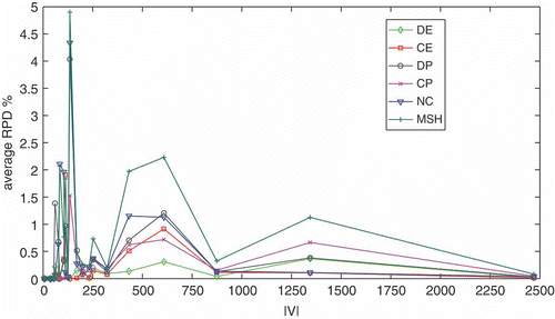
First of all, although not specifically highlighted, it is remarkable that every algorithm is able to produce a complete solution, that is, with O₁ = 0, in every run on every instance. This is a very satisfying performance from the point of view of the subject matter experts. From Table 1 it stems that every algorithm proves to be very efficient on the less challenging instances, vis., i1-i3 and s0035-s0054: not only is 0% RPD achieved for all of them, but they actually keep finding a solution with the same (best) cost in every run. In Figure 10, this corresponds to those points, on the left-hand side, where all the lines reach the horizontal axis. At this stage of the analysis, it is not possible to state that there are algorithms dominated by others, although the ACO with the DE pheromone structure achieves the best average results and the tightest standard deviation. Considered on average, the remaining algorithms rank as CE, CP, DP, NC, and MSH, whereas looking at the standard deviation, the order is CP, CE, DP, NC, and MSH. The right-hand side of Figure 10 reinforces the observation that DE, CE, and CP perform better on large-scale instances. Figure 11 shows the average RPD (logarithmic scale) of the various algorithms as a function of running time.

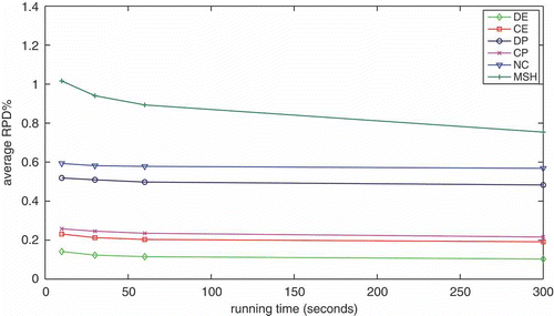
FIGURE 11 Average RPD% as a function of running time.

To gain more insight, it is useful to filter out the simplest instances described and compute the confidence intervals, calling h_is the remaining set of harder instances. Table 2 shows, in the rows, the average RPD (avg) of each algorithm, together with the 95% confidence intervals (lo and up, respectively) and the standard deviation (stdev). For convenience, the same intervals are also plotted in Figure 12.

TABLE 2  Average Results for MSH and ACOs with 95% Confidence Intervals

	lo	avg	up	stdev
MSH	0.42%	1.02%	1.62%	1.27%
DE	0.08%	0.14%	0.20%	0.13%
CE	0.03%	0.26%	0.49%	0.49%
DP	0.19%	0.65%	1.11%	0.97%
CP	0.10%	0.29%	0.48%	0.40%
NC	0.23%	0.77%	1.31%	1.13%

FIGURE 12 Plot of the confidence intervals of Table 2.

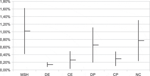
The confidence interval of DE does not overlap with the one associated with MSH, which allows us to conclude that the improvement obtained with the DE pheromone representation is statistically significant. Adding this learning mechanism to the purely random constructive mechanism adopted by the MSH allows us to obtain better results. Interestingly, DE is also better than NC, for which the interval is largely coincident with that of MSH, and this is remarkable: apparently, the clustering information associated with the couple , where T is a tree and v is a node is not powerful enough. The reason cannot depend on the choice of the edge to be inserted in T because, given a node v, the contribution to the objective function is uniquely defined. To understand one possible reason why NC does not perform well, let us consider a graph for which the set of nodes can be partitioned into two disjoint subsets V₁ and V₂, and suppose that it is possible to obtain a solution for which V₁ and V₂ are assigned to trees T₁ and T₂, respectively. Then, a completely equivalent solution can be obtained by swapping the assignments, in other words, by assigning V₂ to T₁ and V₁ to T₂. This kind of representation suffers from the inefficiency because of its embedded strong symmetry: because |K| equivalent solutions can be obtained simply by performing cyclic permutations of the assignments represented in couples c, the algorithm is likely to waste a great deal of CPU time in order to determine which of these equivalent assignments works best.

It can be argued that, at least on the given instances, it is not efficient to represent the clustering information by specifying the tree to which a node must be assigned. Instead, remaining structures try to represent the fact that two or more nodes must be grouped together in a good solution. The performance of DE is superior also to that of DP, even if there is a minimal intersection between the two confidence intervals, whereas the interval of DP is almost entirely contained in that of NC. DE, CE, and CP are then the best configurations. The interval of DE is embedded into that of CE and overlaps for almost its 80% with that of CP, and therefore, no statistical significance of the superiority of DE can be inferred.

We further analyzed the results obtained on h_is instances. The Jarque-Bera test accepted the null hypothesis that the distribution of the RPD obtained by the algorithms comes from a normal distribution at the 1% significance level, but rejects it for DE. We then chose to relax the assumption of normal distribution and performed a Friedman’s test on the results of the pheromone structures (we excluded MSH, which is clearly worse). This test allowed us to reject the null hypotesis that the effects of the columns are zero, because the return value of . It is fair to say that the differences in the performances of the methods are statistically significant. In particular, the mean ranks for DE, CE, DP, CP, and NC are, respectively, 2.2222, 2.3333, 3.4444, 2.8333, and 4.1667. The structures DE, CE, and CP seem to outperform the remaining methods, whereas they do not exhibit relevant diffences among themselves.

Finally, the results from a multiple comparison test are shown in Table 3, which contains a row for each test: the first (alg1) and second (alg2) columns denote the compared algorithms, the fourth (avg) contains the estimated difference in the means between the two, and the third (lo) and fifth (up) columns are the lower and upper bounds of the 95% confidence interval for the true difference of the means. Confidence intervals not crossing zero (highlighted in boldface) mean that the difference is relevant. Here it can be seen that DE and CE are superior with respect to NC, although it cannot be said that they dominate clearly over the others. Moreover, CP is almost better than NC.

TABLE 3  Multiple Comparison Test for Round 1

alg1	alg2	lo	avg	up
DE	CE	−1.5246	−0.1111	1.3024
DE	DP	−2.6357	−1.2222	0.1913
DE	CP	−2.0246	−0.6111	0.8024
DE	NC	−3.3579	−1.9444	−0.5309
CE	DP	−2.5246	−1.1111	0.3024
CE	CP	−1.9135	−0.5000	0.9135
CE	NC	−3.2468	−1.8333	−0.4198
DP	CP	−0.8024	0.6111	2.0246
DP	NC	−2.1357	−0.7222	0.6913
CP	NC	−2.7468	−1.3333	0.0802

Round 2

We performed a second round of experiments to test DE, CE, and CP. We used the harder dataset t, which includes larger-scale instances. Table 4 shows the relative percent deviation from the best solution obtained by the three algorithms. At a first glance, it is possible to argue that the difference in performance of the three methods vanishes when the complexity scale of the instances grows.

TABLE 4  RPD on Instances from Dataset t

ID	BV	DE	CE	CP
rtc.2208.3023.140	0.149	0.01%	0.01%	0.01%
rtc.2217.2088.295	5.307	0.00%	0.00%	0.00%
rtc.2279.2693.177	1.958	0.00%	0.00%	0.00%
rtc.2304.3154.147	0.210	0.00%	0.01%	0.01%
rtc.2329.2175.326	5.539	0.00%	0.00%	0.00%
rtc.2373.2808.181	1.811	0.00%	0.00%	0.00%
rtc.2398.3288.154	0.273	0.01%	0.00%	0.00%
rtc.2400.3288.153	0.201	0.00%	0.00%	0.01%
rtc.2408.2265.327	5.401	0.00%	0.00%	0.00%
rtc.2417.2265.328	5.398	0.00%	0.00%	0.00%
rtc.2475.2925.191	1.906	0.00%	0.00%	0.00%
rtc.2477.2925.191	1.899	0.00%	0.00%	0.00%
rtc.2483.2356.339	5.426	0.00%	0.00%	0.00%
rtc.2499.3425.159	0.182	0.00%	0.00%	0.00%
rtc.2500.3425.160	0.239	0.00%	0.00%	0.00%
rtf.2209.3243.139	0.073	0.01%	0.01%	0.01%
rtf.2304.3384.144	0.006	0.15%	0.06%	0.15%
rtf.2401.3528.151	0.067	0.01%	0.01%	0.01%
rtf.2500.3675.157	0.053	0.02%	0.02%	0.02%
rtp.2246.2980.148	0.521	0.00%	0.00%	0.00%
rtp.2250.2980.147	0.439	0.00%	0.00%	0.00%
rtp.2338.1703.650	7.753	0.00%	0.00%	0.00%
rtp.2338.3094.154	0.517	0.00%	0.00%	0.00%
rtp.2341.3101.154	0.505	0.00%	0.00%	0.00%
rtp.2430.3221.161	0.572	0.00%	0.00%	0.00%
rtp.2430.3224.158	0.393	0.00%	0.00%	0.00%
rtp.2441.2604.235	3.513	0.00%	0.00%	0.00%
average		0.01%	0.01%	0.01%
stdev		0.0003	0.0001	0.0003

Table 5 contains the 95% confidence intervals computed for the three methods on the t dataset, whereas Figure 13 provides a graphical sketch.

TABLE 5  95% Confidence Intervals, t Dataset

	lo	avg	up	stdev
DE	−2.1410^−5	8.661^−5	1.951^−4	2.861^−4
CE	1.3210^−5	5.931^−5	1.051^−4	1.221^−4
CP	−1.4810^−5	9.131^−5	1.974^−4	2.811^−4

FIGURE 13 95% confidence intervals for DE, CE, and DP, t dataset.

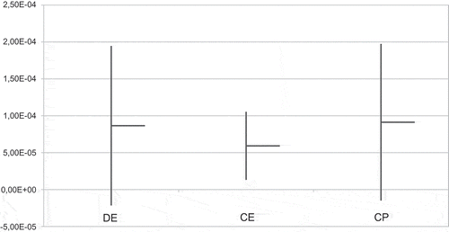
Consistent with the results from the previous round, the Jarque-Bera test shows that the results from DE are not taken from a normal distribution. We executed again a Friedman’s test, whose results established that the differences among the behaviors of these three algorithms are not statistically significant (p = 0.3035) and, in fact, the mean ranks for DE, CE, and CP are 1.7778, 2.1852 and 2.037, respectively, and contrast with the observation of the averages.

A multiple comparison test does not help further in distinguishing the best structure: as shown in Table 6 (which shares the same structure as Table 3), there is no clear predominance.

TABLE 6  Multiple Comparison Test for Round 2

alg1	alg2	lo	avg	up
DE	CE	−1.0334	−0.4074	0.2185
DE	CP	−0.8852	−0.2593	0.3667
CE	CP	−0.4778	0.1481	0.7741

In conclusion, this analysis confirms our initial intuition. As long as problem instances become large (i.e., considering a number of nodes approximately exceeding 1400), the three structures provide mostly equivalent results. On the one hand, if a single pheromone structure had to be selected, then DE would be the best choice, because it is the only one guaranteeing superior performance with respect to that offered by MSH. On the other hand, CE and CP would be the next best alternatives, respectively. Summarizing, these comments allow us to speculate about potentially effective features of pheromone structures, vis.,

• the use of topology, and

• the information about the fact that two or more elements (i.e., nodes, in our case) must belong to the same cluster.

It emerges that DE and CE are characterized by both the features, whereas CP is characterized by just the second one. Finally, it is noteworthy that on the two largest instances, those with 1344 and 2470 nodes, the situation changes, because CE performs the best, and NC and DP close the gap.

These two final observations will be addressed in future research activities.

Conclusions

In this article, five different pheromone structures for an ant colony optimization algorithm have been designed and tested to solve a minimum cost Constrained Spanning Forest problem arising in robot skin design.

The proposed ACO heuristics, namely Direct Edges (DE), Cumulative Edges (DE), Direct Pairs (DP), Cumulative Pairs (DP) and Naive Clustering (NC), have been tested against both real and synthetic instances. Results show the effectiveness of all methods but suggest that some structures work better than others. In particular, the simplest structure (DE) performs definitely better than the simple randomized restart MSH algorithm obtained by disabling the learning capability given by the pheromone and then using the Naive Clustering structure.

DE is superior also to the CP method, but no statistical evidence that DE is better than CE and DP has been found. Moreover, the behavior of the algorithms seems to be sensitive to problem scaling.

Because there is a need, in robot skin design, for automated methods handling an ever-increasing number of sensors per area unit, obtained thanks to miniaturization and technology improvements, even larger cases will be considered in future research activities.

FUNDING

The research leading to these results has received funding from the European Community’s Seventh Framework Programme (FP7/2007-2013) under Grant 231500 (project ROBOSKIN) and 288553 (project CloPeMa).

Notes

1. Please refer to the official iCub website at www.icub.org

REFERENCES

- Alirezarei, H., A. Nagakubo, and Y. Kuniyoshi. 2007. A highly stretchable tactile distribution sensor for smooth surfaced humanoids. In Proceedings of the 2007 IEEE Conference on Humanoid Robotics (HUMANOIDS 2007), 167–173, Pittsburg, PA, USA.
- Allen, P., and P. Michelman. 1990. Acquisition and interpretation of 3-D sensor data from touch. IEEE Transactions on Robotics and Automation 6(4):397–405.
- Anghinolfi, D., G. Cannata, F. Mastrogiovanni, C. Nattero, and M. Paolucci. 2012. Heuristic approaches for the optimal wiring in large-scale robotic skin design. Computers & Operations Research 39(11):2715–2724.
- Anghinolfi, D., G. Cannata, F. Mastrogiovanni, C. Nattero, and M. Paolucci. 2013. On the problem of the automated design of large-scale robot skin. IEEE Transactions on Automation Science and Engineering in press.
- Anghinolfi, D. and M. Paolucci. 2008. A new ant colony optimization approach for the single machine total weighted tardiness scheduling problem. International Journal of Operations Research 5:1–17.
- Argall, B. and A. Billard. 2010. A survey of tactile human-robot interactions. Robotics and Autonomous Systems 58(10):1159–1176.
- Baglini, E., G. Cannata, and F. Mastrogiovanni. 2010. Design of an embedded networking infrastructure for whole-body tactile sensing in humanoid robots. In Proceedings of the 2010 IEEE Conference on Humanoid Robotics (HU-MANOIDS 2010), 671–676, Nashville, TN, USA.
- Bazgan, C., B. Couëetoux, and Z. Tuza. 2011. Complexity and approximation of the constrained forest problem. Theoretical Computer Science 412(32):4081–4091.
- Cannata, G., R. Dahiya, M. Maggiali, F. Mastrogiovanni, G. Metta, and M. Valle. 2010. Modular skin for humanoid robot systems. In Proceedings of the 4th International Conference on Cognitive Systems (CogSys 2010), Zurich, Switzerland.
- Cannata, G., S. Denei, and F. Mastrogiovanni. 2010a. A framework for representing interaction tasks based on tactile data. In Proceedings of the 2010 IEEE International Symposium on Robot and Human Interactive Communication (RO-MAN 2010), 698–703, Viareggio, Italy.
- Cannata, G., S. Denei, and F. Mastrogiovanni. 2010b. Tactile sensing: Steps to artificial somatosensory maps. In Proceedings of the 2010 IEEE International Symposium on Robot and Human Interactive Communication (RO-MAN 2010), 576–581, Viareggio, Italy.
- Cannata, G., S. Denei, and F. Mastrogiovanni. 2010c. Towards automated self-calibration of robot skin. In Proceedings of the 2010 IEEE International Conference on Robotics and Automation (ICRA 2010), 4849–4854, Anchorage, Alaska, USA.
- Cannata, G., M. Maggiali, G. Metta, and G. Sandini. 2008. An embedded artificial skin for humanoid robots. In Proceedings of the 2008 IEEE International Conference on Multi-Sensor Fusion and Integration (MFI 2008), 434–438, Seoul, South Korea.
- Chang, M. C. W., L. Tsao, S. Yang, Y. Yang, W. Shih, F. Chang, S. Chang, and K. Fan. 2007. Design and fabrication of an artificial skin using pi-copper film. In Proceedings of the 20th IEEE International Conference on Micro Electro Mechanical Systems (MEMS 2007), 389–392, Kobe, Japan.
- Cordone, R., and F. Maffioli, 2001. Coloured ant system and local search to design local telecommunication networks. In Proceedings of the 2001 Workshop on Applications of Evolutionary Computing (EvoWorkshop 2001), Lecture Notes in Computer Science 2037, 60–69, Berlin, Heidelberg: Springer.
- Dahiya, R., G. Metta, M. Valle, and G. Sandini. 2010. Tactile sensing: From humans to humanoids. IEEE Transactions on Robotics 26(1):1–20.
- Denei, S., F. Mastrogiovanni, and G. Cannata. 2012. Parallel force-position control mediated by tactile maps for robot contact tasks. In Proceedings of the 2012 IEEE International Conference on Intelligent Robots and Systems (IROS 2012), 3786–3791, Vilamoura, Portugal.
- Dorigo, M., and C. Blum. 2005. Ant colony optimization theory: A survey. Theoretical Computer Science 344:243–278.
- Dorigo, M., and L. Gambardella. 1997. Ant colony system: A cooperative learning approach to the traveling salesman problem. IEEE Transactions on Evolutionary Computation 1(1):53–66.
- Duchaine, V., N. Lauzier, M. Baril, M. Lacasse, and C. Gosselin. 2009. A flexible robot skin for safe physical human robot interaction. In Proceedings of the 2009 IEEE International Conference on Robotics and Automation (ICRA′09), 3676–3681, Kobe, Japan.
- Feder, T., P. Hell, S. Klein, and R. Motwani. 1999. Complexity of graph partition problems. In Proceedings of the 1999 Annual ACM Symposium on Theory of Computing (STOC 1999), 464–472, Atlanta, GA, USA.
- Futai, N., T. Yasuda, M. Inaba, I. Shimoiama, and H. Inoue. 1999. A soft tactile sensor with films of lc resonant traps. In Proceedings of the 1999 IEEE International Conference on Advanced Robotics (ICAR′99), 25–31, Tokyo, Japan.
- Goger, D. and H. Worn. 2007. A highly versatile and robust tactile sensing system. In Proceedings of the 2007 IEEE Conference on Sensors (SENSORS 2007), 1056–1059, Atlanta, GA, USA.
- Gupta, A., J. Lafferty, H. Liu, L. Wasserman, and M. Xiu. 2010. Forest density estimation (Technical Report, Carnegie Mellon University).
- Hakozaki, M., H. Oasa, and H. Shinoda. 1999. Telemetric robot skin. In Proceedings of the 1999 IEEE International Conference on Robotics and Automation (ICRA′99), 957–961, Detroit, Michigan, USA.
- Hakozaki, M. and H. Shinoda. 2002. Digital tactile sensing elements communicating through conducting skin layers. In Proceedings of the 2002 IEEE International Conference on Robotics and Automation (ICRA′02), 3813–3817, Washington, DC.
- Hoshi, T. and H. Shinoda. 2006a. A large area robot skin based on cell-bridge system. In Proceedings of the 2006 IEEE Conference on Sensors (SENSORS 2006), 827–830, Daegu, Korea.
- Hoshi, T. and H. Shinoda. 2006b. A sensitive skin based on touch-area-evaluating tactile elements. In Proceedings of the 2006 IEEE Symposium on Haptic Interfaces for Virtual Environment and Teleoperator Systems, 89–94, Alexandria, Virginia, USA.
- Hwang, E., J. Seo, and Y. Kim. 2007. A polymer-based flexible tactile sensor for both normal and shear load detection and its application to robotics. Journal of Microelectromechanical Systems 16(3):556–564.
- Imielinska, C., B. Kalantari, and L. Khachiyan. 1993. A greedy heuristic for a minimum-weight forest problem. Operations Research Letters 14(2):65–71.
- Jockursh, J., J. Walter, and H. Ritter. 1997. A tactile sensor system for a three fingered robot manipulator. In Proceedings of the 1997 IEEE International Conference on Robotics and Automation (ICRA′97), 3080–3086, Albuquerque, New Mexico, USA.
- Lacasse, M., V. Duchaine, and C. Gosselin. 2010. Characterization of the electrical resistance of carbon-black-filled silicone: Application to a flexible and stretchable robot skin. In Proceedings of the 2010 IEEE International Conference on Robotics and Automation (ICRA′10), 4842–4848, Anchorage, Alaska.
- Lazzarini, R., R. Magni, and P. Dario. 1995. A tactile array sensor layered in an artificial skin. In Proceedings of the 1995 IEEE/RSJ International Conference on Intelligent Robots and Systems (IROS′95), 114–119, Pittsburg, PA, USA.
- Miller, C. E., A. W. Tucker, and R. A. Zemlin. 1960. Integer programming formulation of traveling salesman problems. Journal of the ACM 7:326–329.
- Mittendorfer, P. and G. Cheng. 2011. Humanoid multimodal tactile-sensing modules. IEEE Transactions on Robotics 27(3):401–410.
- Monnot, J., and S. Toulouse. 2007. The path partition problem and related problems in bipartite graphs. Operations Research Letters 35(5):677–684.
- Nagakubo, A., H. Alirezarei, and Y. Kuniyoshi. 2007. A deformable and deformation sensitive tactile distribution sensor. In Proceedings of the 2007 IEEE International Conference on Robotics and Biomimetics (ROBIO 2007), 1301–1308, Sanya, China.
- Nattero, C., D. Anghinolfi, M. Paolucci, G. Cannata, and F. Mastrogiovanni. 2012. Experimental analysis of different pheromone structures in ant colony optimization for robotic skin design. In Proceedings of the 2012 International Federated Conference on Computer Science and Information Systems (FedCSIS 2012), 431–438, Wroclaw, Poland.
- Nilsson, M. 1999. Tactile sensing with minimal wiring complexity. In Proceedings of the 1999 IEEE International Conference on Robotics and Automation (ICRA′99), 293–298, Detroit, Michigan, USA.
- Papadimitriou, C., and K. Steiglitz. 1982. Combinatorial Optimization: Algorithms and Complexity. Upper Saddle River, NJ, USA: Prentice-Hall.
- Schaeffer, S. 2007. Graph clustering. Cluster Science Review 1:27–64.
- Schmitz, A., P. Maiolino, M. Maggiali, L. Natale, G. Cannata, and G. Metta. 2011. Methods and technologies for the implementation of large-scale robot tactile sensors. IEEE Transactions on Robotics 27(3):389–400.
- Shimojo, M. 1994. Spatial filtering characteristic of elastic cover for tactile sensor. In Proceedings of the 1994 IEEE International Conference on Robotics and Automation (ICRA′93), 287–292, San Diego, CA, USA.
- Shimojo, M., T. Araki, A. Ming, and M. Ishikawa. 2010. A high speed mesh of tactile sensors fitting arbitrary surfaces. IEEE Sensors Journal 10(4):822–831.
- Shinoda, H., and H. Oasa. 2000. Wireless tactile sensing element using stresssensitive resonator. IEEE/ASME Transactions on Mechatronics 5(3):258–266.
- Stüutzle, T., and H. Hoos. 2000. Max-min ant system. Future Generation Computer Systems 16:889–914.
- Yan, X., X. Zhou, and J. Han. 2005. Mining closed relational graphs with connectivity constraints. In Proceedings of the 2005 International Conference on Knowledge Discovery and Data Mining (KDD 2005), 324–333, Chicago, Illinois, USA.
- Youssefi, S., S. Denei, F. Mastrogiovanni, and G. Cannata. 2011. A middleware for whole body skin-like tactile systems. In Proceedings of the 2011 IEEE-RAS International Conference on Humanoid Robotics (Humanoids 2011), 159–164, Bled, Slovenia.