A Comparison of Algorithms for Handheld Wand Tracking

Abstract

We examine several algorithms for tracking a handheld wand in a 3D virtual reality system: extended Kalman filters (EKFs), interacting multiple models (IMMs), and support vector machines (SVMs). The IMMs consist of several EKF models, each of which is tuned for one particular type of user motion. For determining the types of motion, we compare hand-created rules with an automatic clustering algorithm, with mixed results. The mode-specific EKFs within the IMM are more accurate than one overall EKF. However, the IMM is comparable to a single EKF, because of the overhead of predicting the current component EKF. SVMs with a one-frame lookahead perform the best, cutting the error in half. Aside from those SVMs, different model types were best for the different dimensions of tracking (x, y, z, and rotation).

INTRODUCTION

Accurate motion tracking is an integral component of interactive augmented and virtual reality systems, allowing a user to control views, navigate through a virtual environment, select and manipulate virtual objects, and realistically animate virtual characters and objects (Welch and Foxlin 2002). Typical systems utilize either a head-mounted or handheld device whose position and orientation is detected by a combination of internal and external reference signals and sensors.

Motion tracking systems are sensitive to noise, which might significantly diminish the user’s experience. Sensors perform more accurately if the target object is stationary and within an optimal distance from the sensor; a fast-moving or distant target could introduce uncertainty into location measurements. Noise can also be introduced by periodic target occlusion, user jitter, or environmental disturbances. Finally, signal processing algorithms can contribute to noise, because tracking systems integrate and process raw physical signals (mechanical, inertial, acoustical, magnetic, or optical) from multiple sensors to generate the final output state (Welch and Foxlin 2002). Thus, a motion tracking system must employ a robust strategy in order to correctly estimate the location and orientation of an object in spite of noisy sample data. Our work examines different methods for performing this estimation.

BACKGROUND

We compare three kinds of estimators: extended Kalman filters (EKFs), interacting multiple models (IMMs), and support vector machines (SVMs).

Extended Kalman Filters

Many motion tracking applications utilize the Kalman filter (Kalman 1960) to reduce noise. The Kalman filter employs a mathematical model of a discrete-time process and knowledge about the system’s prior state to recursively estimate the current state (e.g., location of the target). The estimate is updated or “corrected” with input from an actual observation. The Kalman filter requires linear mathematical models and assumes independent, white Gaussian distributions for the process and measurement noise (Welch and Bishop 2001). When these two conditions are met, the Kalman filter appears to be optimal for minimizing the variance of the estimation error (Maybeck 1979).

However, not all motion patterns can be accurately described with linear models. Various adaptations and alternative filtering mechanisms have been introduced that address nonlinear models. The extended Kalman filter (EKF) replaces the nonlinear process with an approximation. After using a Taylor series expansion to linearize the system about the current state mean and covariances, the EKF applies the standard Kalman filter state estimation and measurement updates (Sorenson 1985). Its disadvantages include the computationally complex derivation of several Jacobian matrices and the tendency of the filter to become unstable when the process model is inaccurate, the process or observation noise is not Gaussian, or linearization time step intervals are not small. As an alternative, the unscented Kalman filter (UKF) represents the current state’s probability distribution (the current mean and covariance estimates) with a minimal set of sample points, which are propagated through the nonlinear model (Julier and Uhlmann 1996). The mean and covariance are reconstructed after the transformation and then the standard Kalman filter is applied. The UKF performs better on highly nonlinear systems than the EKF does, but the improvement appears negligible in cases where the motion models linearize well (LaViola Jr 2003; Saulson and Chang 2003). The particle filter, a sequential Monte Carlo simulation method (Arulampalam et al. 2002), has also been applied to the motion tracking problem and appears to perform comparably to the EKF and UKF for nonlinear orientation estimation (van Rhijn, van Liere, and Mulder 2005); however, it can be computationally expensive and, thus, prohibitive for real-time applications.

Azuma and Bishop (1994) used EKFs to reduce the dynamic registration errors and latency of a head-mounted augmented reality system by predicting head orientation. Their system also predicted translational position with a standard KF. One of their predictors included inertial measurements and the other did not. Three representative motion datasets were studied and both the noninertial and the inertial predictors reduced the average and peak registration errors (4–6 and 10–12 fold, respectively) compared to the raw data for all types of motion.

LaViola Jr. (2003) compared the performance of the UKF to the EKF. Both head and hand orientation were modeled with a quaternion-based constant velocity function. (The “Quaternions” section describes quaternions in more detail.) Both filters performed equivalently, improving tracking accuracy at sampling rates of 80 Hz (22–28% improvement) and 215 Hz (41–47% improvement) over no filter. He concluded that the extra computational demands of the UKF as well as the near-linear nature of the orientation motion favored the use of the EKF.

Van Rhijn, van Liere, and Mulder (2005) analyzed several orientation filtering methods including the EKF, UKF, particle filter (extended and unscented) and linear time invariant filter. Data were obtained from a hand tracking system and included common user hand motions such as object selection, manipulation, tracing, and docking. Synthetic signals containing general characteristics of typical datasets were also incorporated. They used a quaternion-based constant acceleration motion model with inertial measurements, as well as a constant velocity motion model without inertial measurements. The experimental results demonstrated similar performance for the EKF, UKF, and both particle filters.

Based on this existing work, we chose the EKF as the basic filter for estimating position and orientation in our experiments. As the next section describes, our investigation of interacting multiple models (IMMs) extends the work on EKFs for motion tracking to a richer class of models.

Interacting Multiple Models

A multiple model filter (MMF) uses several distinct filters in parallel, which vary in their state estimation models or in the tuning of their process covariance parameters. The MMF combines or selects among their individual outputs to produce the final state estimate.

One type of MMF is an interactive multiple model or IMM (Bar-Shalom and Blom 1988). The IMM applies several filters in parallel, probabilistically transitions between models, computes the likelihood that a given filter correctly models the current motion pattern, and combines the outputs of each filter into a single estimate of the current state. The rest of this section details the operation of an IMM, using the notation of Mazor et al. (1998).

After each observation (i.e., each time step), the IMM computes estimates for the following:

• For each of the n filters, the posterior probability that filter j was active at time k. Let this be μ_j(k).

• For each filter j, an estimate of the state at time k and its covariance P_j(k|k).

When the next observation arrives at time k + 1, there are three steps of the update process for the IMM: interaction, filtering, and combination. During interaction, the for all filters i are combined in a weighted sum to get the “starting state” for filter j. Each filter j uses a different weighted combination, based on the likelihood of switching from one filter to another. As an extreme example, if filter 3 is never active immediately following filter 1, filter 3 will ignore . The formula for is

where μ_i,j(k) is the probability that j is the active filter from time k to k + 1 given that i is the active filter from time k − 1 to k:

The p_ij term is the a priori probability of the system switching from filter i to filter j. We use a stationary Markov chain to model that switching process, so p_ij does not change with time.

In addition to computing the starting state for filter j, the model also computes the covariance of that state:

where c(i,j,k) is the column vector . Computing and P_0j(k|k) for each filter j concludes the interaction step of the update process.

The second step, filtering, runs each component filter j (e.g., an EKF) for one step using the observation at time k + 1. Filter j uses x_0j(k|k) and P_0j(k|k) as if they were its estimates from the previous time step. This produces an estimate of the state at time k + 1 and its covariance P_j(k + 1| k + 1).

The filtering phase is also when the model computes the posterior probability μ_j(k + 1) of filter j being active. Let Λ_j(k + 1) be the likelihood of observation k + 1 according to filter j. Then

The third and final step of updating an IMM is combination. This step computes an overall estimate for the state of the system

and its covariance

where d(j, k + 1) is the column vector

The overall estimates and P(k+1|k+1) are used for prediction and tracking. However, they do not feed back into the IMM at the next time step. Instead, the different state estimates from each filter are combined to feed into the next time step.

When compared to an EKF, the IMM is a more flexible model, because it can model any of several different user behaviors. Our work investigates how that flexibility impacts the accuracy of motion tracking.

Support Vector Machines

Although the EKF and IMM approaches to tracking are both related to Kalman filtering, the SVM approach is fundamentally different. SVMs do not explicitly account for the temporal nature of the data. Rather, they perform regression, learning a function that maps context information to a scalar target value (e.g., x position of the wand). Thus, for our wand-tracking data, each time point is represented by a scalar target value and a d-dimensional feature vector that captures relevant information from that time point. For example, when building an SVM model of the wand’s x position, the target for time i is the actual x position at time i,¹ and the feature vector includes quantities such as the observed x position at time i, the observed x position at time i − 1, the average x position from times i − 10 through i − 2, etc. The training data for the SVM learning algorithm consists of these pairs—feature vector and matching target—for each time step of the training sequence. The learning algorithm (Meyer et al. 2012) takes that data and learns a function to map feature vectors to their respective targets (i.e., regression).

We include a general-purpose regression algorithm (i.e., SVMs) in our experiments in order to compare the EKF-based methods to something fundamentally different. We chose SVMs as our regression method because of their general applicability to a wide range of problems. SVMs compute the estimated target for a new feature vector x based on the targets from some of the training data points, called the support vectors. Training data points that have feature vectors most similar to x carry more weight when making the prediction for x. We use a radial basis kernel to determine “nearness,” as detailed in “SVM Details”. Further details about the SVM algorithm can be found in Bishop (2006), Section 7.1.4. For our purposes, SVMs are simply used as a black-box regression method.

DATA SOURCE

We used an ART TRACKPACK system (ART 2011b) to collect our data. Four infrared cameras are fixed on the top edge of a large projection screen, roughly six feet above and ten feet in front of the user. The cameras were calibrated prior to use. They use a flash (880 nm) to illuminate reflective markers on the tracking wand (a Flystick3 (ART 2011a)) and record an image of the scene. The TRACKPACK system processes the image to produce a 3D wand position and orientation which we collect as a raw data sample.

The noise in the estimated wand position is clearly noticeable when using the system. For example, when a beam is rendered in the environment as if emanating from the wand, the beam jitters considerably, even when the wand is held virtually still. This is partially due to the distance of the user from the screen, which magnifies small errors in tracking the wand’s position and orientation. That magnification underscores the importance of very accurate tracking.

Data samples are collected at a rate of 60 samples per second. Each sample consists of a position—x, y, and z coordinates in millimeters—and an orientation—pitch, yaw, and roll rotation angles in degrees (i.e., Euler angles). Pitch is rotation about the horizontal axis running left and right (i.e., pitch measures angle up and down). Yaw is rotation about the vertical axis (i.e., angle to the left or right). Roll is rotation about the horizontal axis going into/out of the screen.

Quaternions

The rotation angles were converted to quaternion representations prior to passing them to the EKF. Quaternions (Weisstein 2011b, a) are 4D orientation representations (q₀, q_x, q_y, q_z) composed of a rotation angle θ about an axis (q_x, q_y, q_z) where

They are commonly used in place of Euler angles because they are fairly compact, stable, and avoid the singularities of Euler angles. Conversion from Euler angles (α, β, γ) to a quaternion is defined as

Conversion from a quaternion to the Euler angles is given by

Floating point calculations add small rounding errors to a quaternion, which accumulate and eventually lead to values outside the valid domain of several of our functions. Therefore, the quaternions were normalized at various points in the filtering process: immediately after creating the quaternions, at the end of the state update function, and immediately after the orientation estimates were returned by the EKF. Similar normalizations were employed in previous quaternion-based motion tracking studies (LaViola Jr. 2003; Azuma and Bishop 1994).

Evaluation Metric

Reference data were obtained by passing the raw data through a 10-Hz low-pass, finite impulse response (FIR) filter with zero group delay, similar to the method used by van Rhijn et al. (2005). In essence, this smooths the raw data so that radical fluctuations in position, velocity, and acceleration are removed.

The accuracy of each algorithm was measured using a root mean square error (RMSE) metric that compared the estimated states to the reference signal:

where n is the number of time steps and d_i is the error at time step i. For position in the x, y, or z directions, the error d_i (in millimeters) is the difference between the reference value and the estimated value.

For orientation, the error d_i (in degrees) is computed as described in LaViola Jr. (2003), van Rhijn et al. (2005), and Azuma and Bishop (1994). Let be the reference quaternion at time i and let be the estimated quaternion at time i. Then the error at time i is

(1)

The quaternion inverse is defined as

The 0 subscript in Equation (1) indicates that the q₀ component of the corresponding quaternion is the argument to the arccos function.

EKF DETAILS

This section describes the details of the EKF models we used for motion tracking. The description includes our methods for estimating the EKF model parameters, which is a significant part of building an EKF model for an unknown process. Just as this section details our EKF models, the next section gives the details for our IMM models, and “SVM Details” gives the details for the SVM models.

Each EKF we used is described by its type and its level. The type describes which location variable(s) the EKF is responsible for tracking. There are four types: x position (lateral direction); y position (vertical direction); z position (toward/away from the screen); and orientation, which models all three axes of rotation jointly, using a quaternion. Each type of EKF can be set at one of several levels. The level specifies the complexity of the state update function, as described later in this section.

Once the type and level of the EKF are selected, it remains to set the model parameters: the observation function parameters and the state update function parameters. The methods for estimating these parameters for our wand environment are described in the following subsections. We used the Recursive Bayesian Estimation Library (ReBEL) toolkit (van der Merwe and Wan 2012) for Octave (Octave community 2012) to perform the state update for each EKF. The ReBEL toolkit provides a template that we used to specify the state update equations, observation equations, and model parameters for each EKF we used. By following the template, we used the toolkit’s functions for running the models on a data sequence, computing the EKF state estimate at each time step.

A specific EKF model is defined by an observation function, its parameters (i.e., observation noise covariance), a state update function, and its parameters (i.e., process noise covariance). The following subsections describe these aspects of our models.

Observation Function

The observation function relates the noisy state measurements that the tracking cameras “observe” to the true state of the system, accounting for uncertainty in the measurements with an observation noise term:

The observation noise is a zero-mean Gaussian with a state-independent, diagonal covariance matrix.

Estimating the Observation Function Parameters

The variance values for the observation noise were estimated in an offline process. The tracking wand was attached to a tripod, which was placed at 18 different locations throughout the space occupied by a typical user. These locations included positions at different heights, both close and far from the sensor cameras. After setting the wand at a specific location, it was aimed at 9 different points on the screen. For each point, the wand was activated and data were collected for 5 seconds. Because the wand was slightly disturbed when starting each data collection sequence, 2 seconds of data were deleted from the beginning of each sequence. The wand was also disturbed at the end of each collection sequence, but that happened after the 5-second window.

The Euler angles (i.e., pitch, yaw, and roll) of each data point were converted to the quaternion representation prior to calculating the variances. The variances for the x, y, and z coordinate measurements and the q₀, q_x, q_y, and q_z quaternion components were calculated independently. We calculated the sample variance for each variable during each of the 162 data sequences. Each sample variance is an approximation of the observation noise variance because the wand is still during each data sequence. To get an overall estimate for the observation noise variance, we averaged the 162 sample variances. The values we used are as follows: for x, y, z position: 4.51e-3, 2.77e-2, 3.06e-2; for q₀, q_x, q_y, and q_z: 1.24e-7, 5.84e-7, 2.54e-7, and 1.00e-6.

The state update function encodes a set of equations that model a motion pattern using information about the prior state and process noise. The process noise can be viewed as a correction factor that accounts for changes in the state that are not modeled by the state equation. This allows us to use a state update function that is overly simplified when compared to the actual physical process that is occurring, while still yielding reasonable results. Of course, using just one state update function at all times ignores the fact that the user will be moving the wand in many different motions. The IMM approach relieves this constraint (“Interacting Multiple Models”).

To select the state update functions for our models, we individually plotted the x, y, and z positions and the pitch, yaw, and roll versus time and inspected the graphs for dominant motion patterns. Three modes of motion were most apparent for the x, y, and z positions: constant position, constant velocity, and constant acceleration. Similarly, for orientation, we found three basic modes of motion: constant rotation angle, constant rotational velocity, and constant rotational acceleration. These modes led to our three levels of state update functions. The following subsections detail these levels for position and orientation models, respectively.

Position Models

Each position dimension (x, y, z) was modeled independently, using a separate filter. The state of the filter can include information about the position (p), the velocity (v) and the acceleration (a). The process noise w is a zero-mean Gaussian with diagonal covariance matrix. Let w_p, w_v, and w_a represent the components of the noise vector for position, velocity, and acceleration, respectively.

• Constant Position Model (Level 1):

• Constant Velocity Model (Level 2):

• Constant Acceleration Model (Level 3):

Orientation Models

Rotational motion was modeled using quaternions and the methods described by Himberg and Motai (2009). The state of the filter can include information about the orientation (q), the angular velocity (ω) and the angular acceleration (α).

In the constant orientation model, ω and α are not part of the state. In the constant angular velocity model, α is not part of the state. The constant angular acceleration model includes all, q, ω, and α.

Part of the state update involves rotating the orientation. To do this, the current orientation is multiplied by the desired change in rotation, the Δq, which is defined as follows. Let Δt be the time between samples. Then define

Using these, one can compute Δq as

As with the position models, the process noise for the orientation models is a zero-mean Gaussian w. It is composed of the noise terms for orientation, angular velocity, and angular acceleration (w_q, w_ω, and w_α, respectively).

• Constant Position Model (Level 1):

• Constant Velocity Model (Level 2):

• Constant Acceleration Model (Level 3):

Motion patterns can vary for each of the three rotation angles independently. For example, a user may steadily change the yaw while keeping the pitch and roll constant. However, unlike position, we cannot model the rotation angles independently because they are combined into a single quaternion representation in the state. Because each of the three angles can be following each of the three levels (constant orientation, constant angular velocity, or constant angular acceleration), there are 27 possible levels for orientation as a whole. The motion pattern just described would be represented as the constant pitch, constant yaw velocity, and constant roll model, which we call level 121. The first 1 represents the level for the pitch, the 2 is for the yaw, and the last 1 is for the roll. Its state would be five-dimensional: four for the quaternion to represent orientation (i.e., [q₀, q_x, q_y, q_z]) and one for the angular velocity of yaw (i.e., [ω_y]). The other angular velocity components, ω_x and ω_z, would be fixed at 0 in the level 121 model. As another example, model level 312 corresponds to constant acceleration for the pitch, constant position for the yaw, and constant velocity for the roll. It has a seven-dimensional state: [q₀, q_x, q_y, q_z, ω_x, ω_z, α_x].

Estimating the State Update Function Parameters

As noted previously, we used a diagonal covariance matrix for the process noise, so the parameters for the state update function are the diagonal elements of the covariance matrix. The variance values for the process noise are trickier to estimate than for the observation noise because the process itself is hidden. That is, the dataset consists of observations, not process states. Thus, we used numerical optimization to tune the parameters for the process noise.

We trained several EKFs of different types and levels on different subsets of the data (“Models for Comparison”). For each EKF, we used BFGS (Broyden 1969; Fletcher 1970; Goldfarb 1970; Shanno 1970) to numerically optimize the parameters by minimizing the RMSE on the training data. Specifically, we used the bfgsminbfgsmin function in the optimoptim package for Octave (Octave community 2012). We ran the algorithm with weak convergence checks, which checks only the function value for convergence and not the gradient or parameters. This sped up convergence while sacrificing little accuracy.

Similarly to other gradient descent-like algorithms, BFGS is not guaranteed to find the globally optimal parameter values. Instead, BFGS starts with some random initial values for the parameters, then incrementally improves them by adjusting the values a small amount until no more small adjustments result in improved RMSE. When this convergence occurs, BFGS has found an approximate local minimum of the RMSE function.

For each EKF that we trained, we ran BFGS starting from 15 different initial parameter values. These “random restarts” help to avoid particularly bad starting parameters, which can lead to convergence at bad local minima (Bishop 2006, e.g.). Each of the 15 restarts runs independently, converging to a different set of parameter values.

We would like BFGS to find parameters that work well for data in general, not just for the particular data with which it is training and optimizing the error. Finding parameters that work well for the training data but generalize poorly to other data is overfitting, which is a general concern with machine learning algorithms. One technique to mitigate the effects of overfitting is to use validation data: data that is independent from the training data. The training data is given to BFGS for optimization, but the validation data is used separately to check that BFGS is not overfitting. By evaluating candidate parameter values on validation data instead of just the training data, one can estimate how well the parameters will work on new data. We computed the validation RMSE every 10 iterations of BFGS and at convergence, recording the parameter values and RMSE. To pick the final parameters, we selected the recorded parameters that had the lowest validation error. These might or might not be the parameters at convergence, because convergence looks at training set error, whereas the final parameter selection is based on validation error. The final parameter selection was across all 15 restarts, so the final parameters correspond to the best validation error seen in any of the restarts.

If the validation error crept too high, we stopped BFGS, even if it had not converged. Specifically, we triggered early stopping if the validation error was greater than minErr + 0.25(maxErr – minErr), where maxErr and minErr are the highest and lowest validation error values seen so far. In other words, if the error was more than 25% of the way back toward the worst validation error, the algorithm was deemed to be overfitting, so it was stopped.

IMM DETAILS

The EKF process models described in “State Update Function” describe either constant-position motion, or constant-velocity motion, or constant-acceleration motion. However, as the users interact with the system, they will switch among these types of motion. The idea of an IMM is to probabilistically switch among several component filters, based on the type of motion that is currently being observed. An IMM is defined by

• the number of component models,

• the parameters for each component model, and

• the switching parameters, which define how the process switches among the types of motion.

Each component model is built to model a different mode of motion. The next section describes the two methods we investigated for determining the modes of motion. The section that follows that describes how we learn an IMM model, given some definitions for the modes of motion.

Segmenting into Modes of Motion

A segmentation algorithm simply labels each time step of a data sequence with some mode of motion. Implicitly, the segmentation algorithm defines the different modes of motion, as well as how many modes there are. We investigated two different segmentation algorithms, one that uses human intuition and hand-tuned rules and one that uses machine learning to cluster the data into different modes.

Segmenting with Manual Rules

Based on our observations about the data, our rule-based segmentation algorithm uses three types of motion as the possible labels: constant position, constant velocity, and constant acceleration. The labeling was done independently for each of the x, y, and z coordinates and pitch, yaw, and roll rotation angles. Thus, each time step has six category labels: three for the position and three for orientation.

For each of those 6 dimensions, the process for labeling time step t involves calculating some features of the data in a window around time t. Using a 30-time step range, centered on t, we calculated

• the average velocity,

• the average acceleration,

• the path-distance, defined as the length of the path traveled over the course of the 30 time steps,

• and the displacement, defined as the distance between the first and 30th time step positions.

Data samples (i.e., each time step of the data) were initially split into two groups using the ratio of displacement to path-distance. A data sample with a value below threshold c₁ was assigned to the constant position (orientation) group; data above the threshold were assigned to the constant velocity group. At this point, constant acceleration data were still intermingled with both groups.

To further refine the constant position group, a data point was labeled constant position only if its average velocity was below a velocity threshold c₂; otherwise, it was labeled constant acceleration. Likewise, to refine the constant velocity group, a data point was labeled constant velocity only if its displacement/path-distance ratio threshold was below displacement/path-distance ratio threshold c₃; otherwise, it was labeled constant acceleration. The threshold values were individually chosen for each translational (x, y, or z) and rotational (pitch, yaw, or roll) axis of motion through a combination of trial and error and visual inspection of a graph of the position or orientation values versus time superimposed with the group assignments. Threshold values are listed in Table 1.

TABLE 1 Partitioning Thresholds

	X position	Y position	Z position	Pitch	Yaw	Roll
c1	0.99	0.99	0.99	0.20	0.85	0.25
c2	0.005	0.025	0.005	0.0005	0.00009	0.00015
c3	0.0	0.0	0.0	0.80	0.0	0.70

This process was performed for each dimension (three position and three orientation) of each time step. Subsequently, the three orientation labels were combined into one composite label that incorporated the individual Euler angle assignments. For example, constant pitch, constant yaw velocity, and constant roll labels were combined to form label 121. This labeling matches the levels of the orientation models we use for EKFs. Five orientation patterns each occurred less than 0.55% in the dataset, so we eliminated them and reassigned the associated data to a related mode: 112 → 113, 132 → 133, 211 → 212, 221 → 222, 231 → 232.

Thus, at the end of this process, each time step had one of three labels for x position, for y position, and for z position, and one of 22 labels for orientation.

Segmenting Using Clustering

Our second algorithm for segmenting the data is K-means clustering (MacQueen 1967). K-means is a method for grouping data points into similar groups or clusters. As with the rule-based segmentation, the result of this segmentation algorithm is a set of labels for each time step of the data: one label for the orientation mode, and one for each of the x, y, and z position modes. Those labels are computed independently from each other.

To pass the data into K-means, we represent each time step t as some d-dimensional feature vector. Each feature captures the distance moved some time before or after t, with different features corresponding to different amounts of time. For example, consider the case when we are assigning the x-position label, and let x_t be the observed x position at time t. Each feature for time step t takes the form

(2)

Different values of “start” and “end” define different features, which look at different windows of time.

We used two different feature sets for clustering. Feature set 1 had the following (start, end) pairs:

These 15 features look back from t by 4.27 seconds and forward from t up to 0.53 seconds, with the window sizes for the features increasing as you look further in the past or further in the future. Note that we can look forward because the clustering is used only for training the model, not during tracking. During training, we have access to the whole batch of data, including the information after time t. Having more features near the current time means that more emphasis is given to that information closest to the current time.

Feature set 2 is similar, but it examines a smaller window of time. Its (start, end) pairs are {(64, 33), (32,17), (16, 9), (8, 5), (4, 3), (2, 2), (1,1), (−1, −1), (−2, −2), (−3, −4)}. These 10 features look backward from t 1.07 seconds and forward from t 0.07 seconds.

The features for the y and z positions are analogous to the x position features. For orientation, the features are also similar, except, all three axes of rotation are included in one feature vector. Thus, feature set 1 has 3 * 15 = 45 features for orientation, and feature set 2 has 3 * 10 = 30 features.

Each feature was scaled and centered so that it had a sample standard deviation of 1.0 and mean of 0.0. This helped to ensure that features with high variation (e.g., those that measure movement from further back in time) did not artificially dominate the other features simply because of differing scales.

Once we encoded the training data using one of our two feature sets, we had a set of d-dimensional feature vectors, one for each time step. The K-means algorithm uses that training data to find clusters, which are represented by their means. To label other data (e.g., testing or validation data), each time step is assigned the label corresponding to the closest cluster center, where closest is measured using Euclidean distance.

There is one user-selected parameter for the clustering algorithm: K, which determines how many clusters to create. We tried different values of K, from 2 to 15. After examining how the average distance to clusters’ centers varies with K, we chose K = 15 for orientation and K = 8 for each of the position dimensions. These values were for both feature set 1 and feature set 2.

Learning an IMM

As noted earlier, an IMM is defined by the number of component models, the parameters of each component model, and the switching parameters. This section describes our process for learning those pieces, given some method of segmenting the data into different modes of motion.

The number of component models is determined by the segmentation: one for each mode of motion. Each component model is an EKF of some type and level (detailed in “Models for Comparison”), which needs the observation and process covariance parameters specified. The observation covariance parameters are the same as those for a single EKF model of the whole system. The process covariance parameters are learned in the same way as for a single EKF, using BFGS optimization. However, because the EKF is a component within the IMM for some motion mode j, BFGS is given only the time steps of the training data for which the mode of motion is j.

We model the switching between modes as a stationary Markov chain. That is, given that the system is in motion mode i at time t, the probability p_ij of switching to mode j at time t + 1 is independent of t and is independent of anything that happened before time t. For a model with n modes of motion, the switching parameters are {p_ij : ∀1 ≤ i ≤ n, 1 ≤ j ≤ n}. We estimate these using maximum likelihood:

“Interacting Multiple Models” described how these switching parameters are used in the IMM. That description assumes that all of the component models in the IMM have the same state representation. However, in our case, we will be using EKFs of different levels as component models, which have different sized state vectors. To deal with this issue, we internally convert the state representations to the superset of state variables, those for the level-3 (or 333) model. This common state format includes all position (or orientation) values, velocity values, and acceleration values. For lower-level models, some of these values are set to 0 when expanding their state. For example, a constant-velocity x-position model will have position and velocity in its state, but not acceleration. Internally, we append a 0 for acceleration to its state to expand it to the common format that all component models can share. If a high-level model (e.g., constant acceleration) needs to communicate its state to a low-level model (e.g., constant position), then the extra information is discarded by the low-level model.

SVM DETAILS

Although the EKF and IMM approaches to tracking are both related to Kalman filtering, the SVM approach is fundamentally different. SVMs do not explicitly account for the temporal nature of the data. Instead, they use a d-dimensional feature vector to capture information about a given point in time, using that feature vector to estimate the current state.

We explored several feature sets for the SVM. Each feature takes the same form as in Equation (2) (i.e., distance moved since different times in the past or future). The start and end values for each feature set are as follows:

• Feature set 1: {(256, 129), (128, 65), (64, 33), (32, 17), (16, 9), (8, 5), (4, 3), (2, 2), (1, 1)}

• Feature set 2: {(32, 17), (16, 9), (8, 5),(4,3), (2, 2), (1, 1), (−1, −1), (−2, −2)}

• Feature set 3: {(32, 17), (16, 9), (8, 5),(4,3), (2, 2), (1, 1), (−1, −1)}

• Feature set 4: {(32, 17), (16, 9), (8, 5), (4, 3), (2, 2), (1, 1)}

The negative start and end values in feature sets 2 and 3 correspond to observations in the future (i.e., after time t). Thus, in order to use the SVM method with feature sets 2 or 3 in practice, we would need to delay for 1/30 or 1/60 second, respectively, before generating the estimate for state. Although this delay is not desirable, we will see that it might be worthwhile in order to significantly improve the accuracy of the tracker.

Each feature was scaled to have zero mean and standard deviation of 1.0. Given a feature set, the SVM learning algorithm takes the training data and constructs a model that maps the feature values to an estimate for state. Each position dimension (x, y, and z) is modeled independently. For orientation, we have one model for each Euler angle, but each model uses all of the orientation features as inputs.

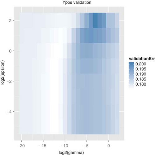
We used the e1071 library (Meyer et al. 2012) for R (R Core Team 2013) to build and evaluate the SVMs. The type of SVM was epsilon-regression, using a radial basis kernel. We explored many possible values of the kernel width parameter γ and the ε parameter. The ε value controls the sensitivity to errors, trading off simplicity of the model (i.e., number of support vectors) for accuracy. We used error on a validation dataset to pick the values for γ and ε. For example, Figure 1 shows the validation error we used to pick the parameters for the y-position predictor with feature set 4. After looking at our initial ranges for ε and γ, if the best value was near an edge of that range, we explored further in that direction. Thus, our final choices for ε and γ were always in the interior of the ranges we explored. The final values for each of the six types of model and for each feature set are listed in Table 2.

FIGURE 1 Validation error for several parameter settings.

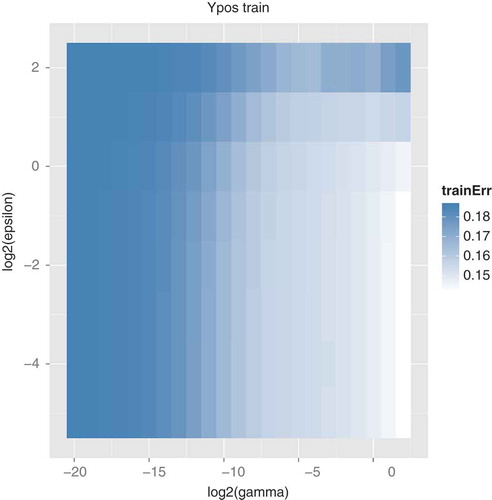
Figure 2 shows the error on the training data for the y-position model with feature set 4. Contrasting this with the error on the validation data (Figure 1) shows the importance of using the validation data. If we had used only the training data to evaluate error, then low ε and high γ will always be best. However, in order to generalize to new data, a smaller γ is needed.

FIGURE 2 Training error for several parameter settings.

EXPERIMENTS

In this section, we describe our experiments comparing EKFs, IMMs, and SVMs for tracking the handheld wand’s position and orientation.

TABLE 2 Parameters for SVM Models

	X Position	Y Position	Z Position	Pitch	Yaw	Roll
Feature set 1	−10, −1	−12, 0	−10, 0	−20, −2	−14, 0	−15, 2
Feature set 2	−2, −3	−6, −3	−4, −3	−20, −2	−8, −3	−9, −2
Feature set 3	−2, −3	−6, −3	−9, −3	−14, −3	−8, −3	−9, −3
Feature set 4	−10, −2	−12, −1	−10, −1	−20, −3	−15, −2	−15, −3

The first number in each cell is log₂ γ and the second is log₂.

The Dataset

We collected data from three subjects using the wand in three applications. Each application used 3D stereoscopic vision to give the user the perception of depth. One application consisted of several cubes distributed in a 3-dimensional space. The wand was used to select cubes and move them to different locations. The second application was a visualization of a liver, in which the user could zoom in and out and investigate the vascular system in the liver. The third application was a simulation of wind around a moving car, with which the user could see the disruptions in air flow and turbulence, using the wand to highlight notable areas. In all three cases, the user moved the wand with a variety of motions. These included holding the wand steady while pointing to a specific location on the screen; moving the wand at various speeds from one point to another, following both straight and curved paths; and moving the wand in a more refined path as though tracing an object.

The data was partitioned into three subsets: training, validation, and testing. Because we want to find tracking methods that work across applications, our testing data includes data from two applications (liver and car) not used in the training or validation data. Similarly, we want tracking methods that work across different users, so the testing data includes data from a user that is not represented in the training or validation sets. The fact that the testing set includes data from unseen applications and new users is an important quality for measuring how well the tracking methods will perform in a variety of scenarios.

The training data consists of 20188 time steps of data (approximately 5.5 minutes). The validation data consists of 27279 time steps of data (approximately 7.5 minutes). The test data consists of 64805 time steps of data (approximately 18 minutes).

Models for Comparison

We evaluated the tracking accuracy of the following models:

• Raw observations: As a baseline, we measured the accuracy of a “model” that simply echoes the observation as the state estimate.

• Single EKFs: Each of these models is a single EKF trained on all of the training data. We trained one EKF of each level: constant position, constant velocity, and constant acceleration.

• IMMs: We evaluated several IMMs, which differ in the segmentation algorithm used for training the component EKFs and the levels of the component EKFs.

  1. Using the hand-tuned rules for segmentation, we built an IMM in which all of the component EKFs were level 1; another IMM in which all of the component EKFs were level 2; and another with all level-3 components. In addition, we built an IMM in which the level of each component matches the type of motion to which it was assigned. For example, the component that was trained on the time steps labeled as constant velocity would be a level-2 model.

  2. We also constructed IMMs using the clustering-based segmentation. Based on our initial experiments, the level-2 models were generally performing the best, so we learned IMM models in which all of the EKF components were level 2. In addition, for modeling the y position, we built an IMM with all level-3 components, because level-3 models showed promise for modeling the y position. These IMMs were constructed for each of the two feature sets used in clustering.

• SVMs: Each of the four feature sets described in “SVM Details” produces a different SVM model.

Results

Figure 3 shows the RMSE on the testing data for each model, sorted by the error. The shading indicates the category of model. Figure 4 shows the same information, except it is sorted by the category of model, and Table 3 presents the same numbers in table form. In those figures and table, “SVMi” indicates the SVM model using feature set i. Similarly, the “Ci” indication for some of the IMM models indicates that segmentation was done with clustering using feature set i. IMM labels without a “Ci” used the rule-based segmentation.

TABLE 3 Error of the models on the test data, sorted by model

	Orientation	X Position	Y Position	Z Position
SVM4	0.200898	0.152526	0.189350	0.140413
SVM3 (delay one step)	0.095039	0.081785	0.089941	0.071463
SVM2 (delay two steps)	0.150942	0.082322	0.090996	0.064607
SVM1 (long history)	0.200667	0.152836	0.191033	0.142049
Raw observation	0.210939	0.156854	0.199818	0.150396
One EKF, Level 3	0.201370	0.156840	0.183630	0.138250
One EKF, Level 2	0.179360	0.153610	0.189040	0.139170
One EKF, Level 1	0.198780	0.156480	0.199920	0.149920
Known Modes, Multiple Levels	0.186700	0.151100	0.186190	0.142290
Known Modes, Level 3	0.184170	0.150510	0.184230	0.142710
Known Modes, Level 2	0.176250	0.150870	0.185500	0.140810
Known Modes, Level 1	0.185120	0.154580	0.193240	0.149490
Known Modes, C2, Level 3			0.182430
Known Modes, C2, Level 2	0.179420	0.146840	0.184680	0.134330
Known Modes, C1, Level 3			0.178050
Known Modes, C1, Level 2	0.170890	0.147620	0.180590	0.136290
IMM, Multiple Levels	0.197590	0.153610	0.189870	0.143890
IMM, Level 3	0.197800	0.153800	0.186460	0.142570
IMM, Level 2	0.187670	0.153900	0.188720	0.139950
IMM, Level 1	0.198470	0.158740	0.196680	0.147270
IMM, C2, Level 3			0.191710
IMM, C2, Level 2	0.192250	0.153790	0.190650	0.138860
IMM, C1, Level 3			0.187990
IMM, C1, Level 2	0.190700	0.154770	0.189750	0.142760

Italics highlight noteworthy results: the raw observation error, which is our baseline error, and the model that achieves the lowest error for each dimension.

FIGURE 3 Error of the models on the test data, sorted by error.

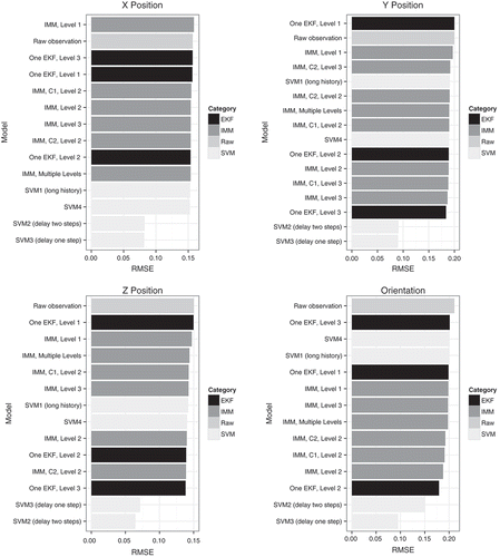
FIGURE 4 Error of the models on the test data, sorted by model.

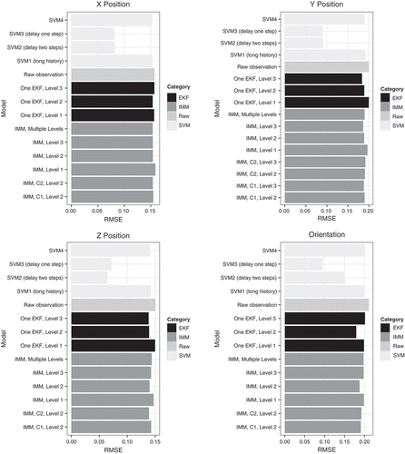
For each type of model—x position, y position, z position, and orientation—predicting the raw observation leads to the worst or second worst error (Figure 3). Thus, EKFs, IMMs, and SVMs are each an improvement over no model.

The most noteworthy result is the vast improvement when using SVMs with a one-step delay (i.e., 1/60 second), which is the best model for orientation, x position, and y position, and the second-best model for z position (Figure 3). In fact, the SVM with one-step delay reduces the error for x position by 48%, for y position by 55%, for z position by 52%, and for orientation by 55%, when compared to the raw observation error. Delaying for a second time step leads to only a slight improvement for z position tracking; for the other model types, two-step delay is slightly worse than one-step delay.

Among the other models, the level-1 models are consistently among the worst models. Among the IMM models, there is little consistency across the types of models, suggesting that motion in the different dimensions has different tendencies. For modeling the x position, the IMM with rule-based segmentation and component models of different levels is best. For modeling the y position, the IMM with rule-based segmentation and component models of level 3 is best. For modeling the z position, the IMM with clustering segmentation and level-2 components is best. For orientation, the IMM with rule-based segmentation and level-2 components is best.

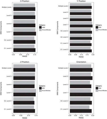
Comparing IMMs with single EKFs, we find that only when modeling x position is the best IMM better than the best single EKF, and even that difference is very slight. This was somewhat surprising, so we investigated the IMMs further. Part of the challenge for an IMM model is to infer the current mode of motion from the observations. To evaluate the degree to which that mode estimation contributed to the model error, we ran each IMM while providing it the correct mode of motion. That is, the model did not have to infer the mode, but that information was provided along with the observation. We call this a “Known Modes” model. Although knowing the mode is not a realistic usage scenario, it helps to diagnose the source of errors in the IMMs’ predictions. Figure 5 plots the error from each “Known Modes” model with the error for each corresponding IMM (which had to infer the modes). For orientation, x position, and y position, all of the IMMs have lower error when provided the modes, whereas for z position, a few of the IMMs show such a drop. For all four types of models, the component models of the IMMs are indeed more accurate than the single EKF models. However, the added complexity of inferring the mode of motion makes the IMMs’ error comparable to a single EKF (Figure 3).

FIGURE 5 Error of the IMM models, with and without known modes.

SUMMARY

We compared several methods for tracking the position and orientation of a handheld pointing device: single EKF models, IMM models composed of several EKFs, and SVMs, which do not explicitly model the temporal nature of the data. All of these methods are improvements over simply using the most recent observation as the estimated position. We thoroughly investigated IMMs, based on the theory that the IMM’s different component models would fit well with the different types of user motion. Although the specialized component models within the IMM did achieve lower error than a single EKF for the whole system, the added complexity of inferring which component model to use at each time step renders the overall IMM error comparable to that of a single EKF model. Thus, although IMMs have some intuitive appeal, the wide range of IMMs that we tested did not provide a benefit over a single EKF model.

The most accurate model by far came from using SVMs with a delay of 1/60 second. That delay allows the SVMs to use one additional observation as a data feature, which cuts the error in half. Although this drastic reduction in error comes at the cost of delaying the position estimation, that delay is very small (i.e., one screen refresh cycle on a 60-Hz display). Depending on the application, the delay might not even be noticed by the user. Thus, we expect that many applications can benefit from improved tracking by using a one-step-delay SVM model.

Notes

¹ See “Evaluation Metric” for how we compute the actual positions.

REFERENCES

- ART. 2011a. Flystick3 wand. Available at http://www.ar-tracking.com/products/interaction-devices/flystick3/.
- ART. 2011b. Trackpack system. Available at http://www.ar-tracking.com/products/tracking-systems/trackpack-system/.
- Arulampalam, S. M., S. Maskell, N. Gordon, and T. Clapp. 2002. A tutorial on particle filters for on-line non-linear/non-Gaussian Bayesian tracking. IEEE Transactions on Signal Processing 50:174–188.
- Azuma, R., and G. Bishop. 1994. Improving static and dynamic registration in a see-through HMD. Proceedings of SIGGRAPH 1994, 197–204. Orlando, Florida, 24–29 July.
- Bar-Shalom, Y., and H. A. P. Blom. 1988. The interacting mutiple model algorithm for systems with Markovian switching coefficients. IEEE Transactions on Automatic Control 33:780–783.
- Bishop, C. M. 2006. Pattern Recognition and Machine Learning. Berlin: Springer.
- Broyden, C. G. 1969. A new double-rank minimization algorithm. Notices of the American Math Society 16:670.
- Fletcher, R. 1970. A new approach to variable metric algorithms. The Computer Journal 13(3):317–322.
- Goldfarb, D. 1970. A family of variable-metric methods derived by variational means. Mathematics of Computation 24:23–26.
- Himberg, H., and Y. Motai. 2009. Head orientation prediction: Delta quaternions versus quaternions. IEEE Transactions on Systems, Man and Cybernetics–Part B 39:1382–1392.
- Julier, S., and J. Uhlmann. 1996. A general method for approximating nonlinear transformations of probability distributions. Technical report. University of Oxford.
- Kalman, R. 1960. A new approach to linear filtering and prediction problems. Transactions of the ASME–Journal of Basic Engineering 82:35–45.
- LaViola Jr., J. J. 2003. A comparison of unscented and extended Kalman filtering for estimating quaternion motion. Proceedings of the 2003 American control conference 3:2435–2440. IEEE.
- MacQueen, J. B. 1967. Some methods for classification and analysis of multivariate observations. In Proceedings of the Fifth Berkeley Symposium on Mathematical Statistics and Probability, Vol. 1:281–297. Berkeley, CA: University of California Press.
- Maybeck, P. S. 1979. Stochastic models, estimation, and control, Vol. 1. Lake City, UT: Academic Press, Inc.
- Mazor, E., A. Averbuch, Y. Bar-Shalom, and J. Dayan. 1998. Interacting multiple model methods in target tracking: a survey. IEEE Transactions on Aerospace and Electronic Systems 34(1):103–123.
- Meyer, D., E. Dimitriadou, K. Hornik, A. Weingessel, and F. Leisch. 2012, Sept. e1071. Available at http://cran.r-project.org/web/packages/e1071/index.html.
- Octave community. 2012. GNU/Octave. Available at http://www.gnu.org/software/octave/.
- R Core Team. 2013. R: A language and environment for statistical computing. Vienna, Austria: R Foundation for Statistical Computing. Available at http://www.R-project.org
- Saulson, B., and K. C. Chang. 2003. Comparison of nonlinear estimation for ballistic missile tracking. Signal Processing, Sensor Fusion, and Target Recognition XII, Proceedings of the SPIE 5096: 13–24.
- Shanno, D. F. (1970). Conditioning of quasi-Newton methods for function minimization. Mathematics of Computation 24:647–656.
- Sorenson, H. W. 1985. Kalman filtering: Theory and application. IEEE Press.
- van der Merwe, R., and E. A. Wan (2012). ReBEL Toolkit. Available at http://web.cecs.pdx.edu/~ericwan/rebel-toolkit.html.
- van Rhijn, A., R. van Liere, and J. D. Mulder. 2005. An analysis of orientation prediction and filtering methods for VR/AR. Proceedings of the 2005 IEEE Conference on Virtual Reality (VR ’05), 67–74. Germany, 12–16 March.
- Weisstein, E. W. 2011a. Euler parameters. From MathWorld–A Wolfram Web Resource. Available at http://mathworld.wolfram.com/EulerParameters.html.
- Weisstein, E. W. 2011b. Quaternion. From MathWorld–A Wolfram Web Resource. Available at http://mathworld.wolfram.com/Quaternion.html.
- Welch, G., and G. Bishop. 2001. An introduction to the Kalman filter (Technical Report 95-041 University of North Carolina, Department of Computer Science).
- Welch, G. and E. Foxlin 2002. Motion tracking: No silver bullet, but a respectable arsenal. IEEE Computer Graphics and Applications 22:24–38.