Stellar-Mass Black Hole Optimization for Biclustering Microarray Gene Expression Data

Abstract

DNA microarray gene expression data analysis has provided new insights into gene function, disease pathophysiology, disease classification, and drug development. Biclustering in gene expression data is a subset of the genes demonstrating consistent patterns over a subset of the conditions. The proposed work finds the significant biclusters in large expression data using a novel optimization technique called stellar-mass black hole optimization (SBO). This optimization algorithm is inspired from the property of the relentless pull of a black hole’s gravity that is present in the Universe. The proposed work is tested on benchmark optimization test functions and gene expression benchmark datasets, and the results are compared with swarm intelligence techniques such as particle swarm optimization (PSO), and cuckoo search (CK). The experimental results show that the SBO outperforms PSO and CK.

INTRODUCTION

Microarray technology attracts keen interest among the scientific community and in industry. Through an analysis of gene expression data, it is possible to learn the behavioral patterns of genes such as similar behavior (Lockhart and Winzeler 2000). These patterns are used in the medical domain to aid in more accurate diagnoses, treatment planning, and drug discovery. DNA microarray enables researchers to analyze the expression of many genes in a single experiment rapidly and in an efficient manner. After the number of preprocessing steps, the low-level analysis of a microarray can be represented as a numerical matrix. In this matrix, the rows represent different genes and the columns represent experimental conditions (Androulakis, Yang, and Almon 2007). Each element of the matrix represents the expression level of a gene under a specific condition, which is represented by a real number. Figure 1 shows the gene expression data matrix.

FIGURE 1 Gene expression data matrix. © Mark Reimers/Exploratory Analysis. Reproduced by permission of Mark Reimers/Exploratory Analysis. Permission to reuse must be obtained from the rightsholder.

Analysis via clustering makes several assumptions that might not be completely adequate in all situations. First, the clustering can be applied to either genes or conditions; it implicitly directs the analysis of a particular aspect of the system. Second, clustering algorithms usually seek a disjoint set of elements, requiring that no gene or sample belongs to more than one cluster. Biclustering is a simultaneous clustering of both the rows and columns of gene expression data. The problem of partitioning of a set of objects into k groups, which optimizes a stated condition of partition adequacy, is not given as straightforward. Given n objects, the number of ways in which these objects can be partitioned into k nonempty subsets (Liu 1968) is given in Equation (1).

(1)

Equation (2) approximates Equation (1):

(2)

Therefore, when the number of clusters k is not known in advance, then the total number of valuations is given in Equation (3).

(3)

Finding significant biclusters in a microarray is a much more complex problem than clustering (Divina and Aguilar-Ruiz 2006) and it is an NP-hard problem (Tanay, Sharan, and Shamir 2002). The search space for the biclustering problem is 2^m+n, where m and n are the number of genes and conditions, respectively. Usually m+n is more than 2000. The problem of finding a consistent biclustering can be formulated as an optimization problem. An optimization problem is a problem that determines the set of potential solutions to the problem and defines one or more criteria that measures the quality of an individual solution. Therefore, our goal is to design and develop an algorithm to find coherent biclusters from gene expression data by using an optimization technique. Hence, we design and implement the biclustering based on the new optimization technique named stellar-mass black hole optimization (SBO). There are probably millions of stellar-mass black holes in our Milky Way galaxy. They trap stars, gas, planets, and anything else that would get up close. The strength of gravity of a black hole depends on the mass of the object and the distance from it. When it absorbs matter, the mass of the black hole is increased; during radiation its mass is decreased. The optimization technique is deduced based on the physics properties of a black hole.

The remainder of this article is organized as follows: in “Biclustering” we describe the structure of biclusters, the problem statement, and a brief introduction to related works in biclustering. The next section describes a general overview of the black hole and SBO. A performance comparison of the SBO with the PSO and CK is presented and a “Biological Analysis Of Biclusters,” followed by our conclusion.

BICLUSTERING

Biclustering is a powerful analytical tool for the biologist. Biclustering methods perform clustering in two dimensions simultaneously. That means clustering methods derive a global model and biclustering algorithms produce a local model. When clustering is applied to gene expression data, genes as well as conditions can be clustered. However, each gene in a bicluster is selected using only a subset of the conditions, and each condition in a bicluster is selected using only a subset of the genes. Biclustering, thus, performs simultaneous clustering of both rows and columns of the gene expression matrix instead of clustering these two dimensions separately. In short, unlike clustering algorithms, biclustering algorithms can identify groups of genes that show similar activity patterns under a specific subset of the experimental conditions. Biclustering is used when one or more of the following situations apply (Madeira and Oliveira 2004):

1. A single gene may participate in multiple pathways that may or may not be coactive under all conditions.

2. Only a small set of the genes participate in a cellular process of interest.

3. An interesting cellular process is active only in a subset of the conditions.

Structure of Biclusters

Several types of biclusters have been described and categorized in the literature, depending on the pattern exhibited by the genes across the experimental conditions (Mukhopadhyay, Maulik, and Bandyopadhyay 2010). Madeira and Oliveira (2004) have identified four major groups of structures inside the submatrices:

1. Bicluster with constant value:

2. Bicluster with constant values on rows or columns:

3. Bicluster with coherent values:

4. Bicluster with coherent evolutions:

The bicluster sets are classified according to their relative structure (Madeira and Oliveira 2004). This structure illustrates the arrangement of the bicluster in full space. Figure 2 shows (a) a Single Bicluster, (b) an Exclusive Row-and-Column Bicluster, (c) a Checkerboard Bicluster, (d) an Exclusive-Rows Bicluster (e) an Exclusive Column Bicluster, and (f) an Arbitrarily Positioned Overlapping Bicluster.

FIGURE 2 Structures of biclusters.

Problem Statement

The gene expression data can be represented as N × M matrix A of real numbers. Let G be a set of genes, C a set of conditions, and A(G, C) the expression matrix, where G = {1,2, … , m} and C = {1,2, … , n}. The element GEx_i,j of A(G, C) represents the expression level of gene ‘i’ under condition ‘j’. The aim of biclustering is to extract the submatrix A(G’, C’) of A(G, C), which is identified by gene subset G’ of G and condition subset C’ of C. In general, the problem can be defined as finding large sets of rows and columns (volume) such that the rows show unusual similarities along the dimensions characterized by columns and vice-versa. The bicluster cardinality or volume of bicluster is simply the product of the number of genes and number of conditions in the bicluster. Our aim is to discover the biclusters of maximum size with the minimum mean squared residue (MSR) and maximum of gene variance (nontrivial).

Review of Related Works

In recent years, several biclustering methods have been suggested for identifying local patterns in gene expression data. The biclustering algorithms are classified into two different approaches: systematic search algorithms and stochastic search algorithms, also called metaheuristic algorithms. The first biclustering algorithm, called direct clustering, proposed by Hartigan (1972) was one of the first works ever published on biclustering, although it was not applied to gene expression data. Moreover, Cheng and Church (2000) presented a first biclustering approach for gene expression data. Their algorithm adopts a sequential covering strategy in order to return a list of n biclusters from an expression data matrix. It finds a single bicluster at a time; repeated application of the method on a modified matrix is needed to discover multiple biclusters. It results in highly overlapping gene sets, which is a mere drawback. Tanay et al. (2002) introduced a statistical-algorithmic method for bicluster analysis (SAMBA), a biclustering algorithm that performs the simultaneous bicluster identification by using exhaustive enumeration. In this method, the significant biclusters were identified by using a graph theoretic approach in which, because of its high complexity, the number of rows that the bicluster may have is restricted.

Murali and Kasif (2003) intended to find conserved gene expression motifs (xMOTIFs). They defined an xMOTIF as a subset of genes that is simultaneously conserved across a subset of the conditions. In order to prevent the algorithm from finding too small or too large biclusters, some constraints on their size, conservation, and maximality is added to its formal definition. Nevertheless, the algorithm uses prior knowledge about the sample phenotypes. Ben-Dor et al. (2003) defined a bicluster as an order-preserving submatrix (OPSM). The algorithm can be used to discover more than one bicluster in the same dataset, even when they are overlapped. Even so, the model concerns only the order of values and, thus, makes the model quite restrictive. Bergmann, Ihmels, and Barkai (2003) proposed an iterative signature algorithm (ISA) that provides a definition of biclusters as transcription modules to be retrieved from the expression data. This method includes data normalization and the use of thresholds that determine the resolutions of the different transcription modules. However, there is no evaluation of the statistical significance.

Mitra and Banka (2006) presented a multiobjective evolutionary algorithm (MOEA) based on Pareto dominancy. Per the objective of this method, it extracts of a large volume of bicluster to a given threshold, nevertheless, the main drawback is that it consumes much time to find the best bicluster and no overlapping is carried out. Divina & Aguilar-Ruiz (2006) presented a sequential evolutionary biclustering (SEBI) approach. The term sequential refers to the way in which biclusters are discovered; only one bicluster is obtained per each run of the evolutionary algorithm. An advantage of SEBI is that a matrix of weights is used for the control of overlapped elements among the different solutions. Nevertheless, the main drawback of this method is that it works well only for the special case of approximately small biclusters. Liu and Wang (2007) introduced a maximum similarity bicluster (MSB) algorithm. A process of iteratively removing the row or column in the bicluster with the worst similarity score is performed until there is one element left in the bicluster. MSB performs well for overlapping biclusters and works well for additive biclusters; it works for the special case of approximately square biclusters.

DiMaggio et al. (2008) proposed an approach that is based on the optimal reordering of the rows and columns of a data matrix in order to globally minimize a dissimilarity metric. Conversely to OPSM, this approach allows for monotonicity violations in the reordering, but penalizes their contributions according to a selected objective function. However, the main drawback of this method is that the objective function extracts trivial solutions. Liu et al. (2009) based their biclustering approach with the use of a PSO together with crowding distance as the nearest neighbor search strategy, which speeds up the convergence to the Pareto front and also guarantees diversity of solutions. Using PSO has the problems of dependency on initial point and parameters, difficulty in finding their optimal design parameters, and the stochastic characteristic of the final outputs. Coelho, de Franca, and Zuben (2009) presented an immune-inspired algorithm for biclustering based on the concepts of clonal selection and immune network theories adopted in the original aiNet algorithm. It explores a multipopulation aspect by evolving several subpopulations that will be stimulated to explore distinct regions of the search space. Nevertheless, they consider only two different objectives: MSR and volume; it might return trivial biclusters.

Ayadi, Elloumi, and Hao (2012) proposed as a pattern-driven neighborhood search (PDNS) approach to the biclustering problem. It utilizes fast greedy algorithms to generate diversified initial biclusters of reasonable quality and a randomized perturbation strategy. This has the drawback that it results in highly overlapping gene sets. Huang et al. (2012) proposed a new biclustering algorithm based on the use of an evolutionary approach (EA) together with hierarchical clustering. The parallel computing technology would be of great help to speed up the traditional EA framework, but its disadvantage is that it extracts a small volume of biclusters. Roy, Bhattacharyya, and Kalita (2013) introduced a CoBi: a pattern-based coregulated biclustering of gene expression data. It is used mainly for grouping both positively and negatively regulated genes from microarray expression data. However, it returns small size biclusters for large MSR value. Maatouk et al. (2014) proposed an evolutionary biclustering algorithm based on the new crossover method (EBACross). In order to avoid overlapping biclusters and to increase the diversification of biclusters, a mutation operator used. Nevertheless, it possibly takes a very long time on large inputs. Ayadi and Hao (2014) presented a memetic biclustering algorithm (MBA) to discover the negative correlation biclusters. It is used mainly for grouping both positively and negatively regulated genes from microarray expression data. Extracting small biclusters and quality of biclusters depending on threshold values are the main issues of this approach.

STELLAR-MASS BLACK HOLE OPTIMIZATION

Preamble

Using Newton’s Laws in the late 1790s, John Michell of England and Pierre-Simon Laplace of France independently suggested the existence of an invisible star. They calculated the mass and size that an object needs in order to have an escape velocity greater than the speed of light, and around a black hole there is a mathematically defined surface called the event horizon that marks the point of no return. In 1915, the presence of black holes was predicted through Einstein’s theory of general relativity. In 1967, John Wheeler, an American theoretical physicist, applied the term “black hole” for the collapsed objects (Luminet 1998). A black hole is an object that is so compact, its gravitational force prevents anything, including light, from escaping. There are so many black holes in the universe that it is impossible to count them. A black hole is born when an object becomes unable to withstand the compressing force of its own gravity. They form whenever massive but otherwise normal stars die. The black holes cannot be seen but can be detected by material being attracted to and falling into them.

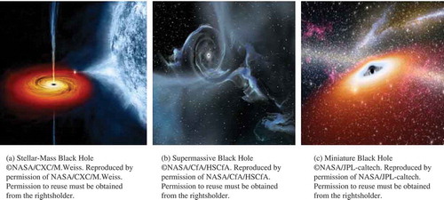
The hole is called “black” because it absorbs all the light that hits the horizon, reflecting nothing, just as a perfect blackbody in thermodynamics. In this way, astronomers have identified and measured the mass of many black holes in the universe through careful observations of the sky. All matter in a black hole is squeezed into a region of infinitely small volume, called the central singularity. The event horizon is an imaginary sphere that measures how close to the singularity an object can safely get. Once an object has passed the event horizon, it becomes impossible to escape: the object will be drawn in by the black hole’s gravitational pull and will be squashed into the singularity. The size of the event horizon is proportional to the mass of the black hole. According to theory, there might be three different types of black holes depending on their mass: Stellar, Supermassive, and Miniature as shown in Figure 3. These black holes would have been formed in different ways. Supermassive black holes, which can have a mass equivalent to billions of suns, likely exist in the centers of most galaxies. The miniature black hole would have a mass much smaller than that of a sun. The miniature black holes could have formed shortly after the big bang.

FIGURE 3 Different types of black holes, based on the mass.

Formation and Evolution of a Stellar-Mass Black Hole

Stellar-mass black holes are born with a bang or when a massive star collapses. When massive stars are collapsed, black holes of up to 10³ solar masses are produced. They form because of a massive star that runs out of nuclear fuel and explodes as a supernova. The rest of the substance is a black hole because the explosion blows much of the stellar material away (Chaisson and McMillan 2008). A single stellar-mass black hole can grow quickly by consuming nearby stars and gas, often in plentiful supply near the galaxy center. The black hole might also merge with other black holes that drift to the galactic center during collisions with other galaxies. The black holes actually evaporate, slowly returning their energy to the universe. While emitting particles, the black hole loses energy and it becomes smaller. Smaller black holes yield more intense radiation than larger ones. The emission continues until the death of the black hole.

Methodology

Based on the Stephen Hawking emission and absorption process, when the black hole absorbs matter, the mass of the black hole is increased; during emission its mass is reduced. Stellar-mass black holes can grow by pulling gas of a companion star that orbits around it. The diet of known black holes consists mostly of gas and dust, which fill the otherwise empty space throughout the universe. Black holes can also consume material torn from nearby stars. In fact, the most massive black holes can swallow stars whole. They can also grow by colliding and merging with other black holes. A black hole gathers any mass, then it grows in mass and slightly in size. The mass decreases via a complicated process called black hole evaporation, or Hawking Radiation, named for Stephen Hawking. Hawking radiation is black body radiation that is predicted to be released by black holes due to quantum effects near the event horizon.

The stellar-mass black hole has the following properties:

• The mass of a black hole grows when it absorbs matter.

• A black hole also grows by colliding and merging with other black holes.

• When emitting particles a black hole loses energy and its mass is reduced.

• Smaller black holes radiate more than larger ones.

• The emission becomes more and more and the black hole is no more.

Based on the above properties, a new optimization technique is devised that incorporates both diversification and intensification in the search space. The individuals succeed to new characteristics that help them survive. The optimization resembles an evolutionary technique, referring to the cumulative changes that occur in a population over time. Table 1 shows the comparison of social strategies with SBO.

TABLE 1 Comparison of Black Hole Socially Relevant Strategies with Optimization

Social Strategy	SBO
Black hole	Feasible solution to the problem
Black hole mass	Fitness value
Black holes in the universe	Population of feasible solution
Emission and absorption of a black hole	Stochastic operators
Progression of populations to suit the universe	Iteratively applying stochastic operators on a set of feasible solutions

The perpetual mystery of the black holes is that they appear to exist on radically different mass scales. There are the countless black holes that are left over from massive stars. These stellar-mass black holes are peppered throughout the Universe and are generally 10 to 24 times as massive as the sun. Scientists estimate that there are as many as ten million to a billion such black holes in the Milky Way alone. For the optimization problem, the initial population of black holes with m dimensions is considered as a candidate solution for the problem. Each black hole is assigned a fitness value according to the solution of the problem.

Evolution

The distance from the surface (or event horizon) of the black hole to the center (or singularity) is called the Schwarzschild radius. This radius is the size that any object would be if compressed enough to form a black hole; it varies from only centimeters across to several kilometers across (Chaisson and McMillan 2008). The Schwarzschild radius increases when the mass of the original object increases but the actual radius does not. It is interesting to mention that the irreducible mass is related to the area A of the event horizon as shown below:

One way to grow a more massive black hole is for a seed black hole in a dense galactic nucleus to swallow up gas and normal stars. It keeps on growing by absorbing mass from its surroundings. By absorbing other stars and merging with other black holes, supermassive black holes of millions of solar masses may form. If two black holes merge together, then their event horizons are contiguous. Figure 4 shows a growth of black hole and collision of two black holes (Luminet 1998).

FIGURE 4 Growth of a black hole.

The growth rate of a black hole is directly proportional to its mass. The higher mass black hole has a higher absorption level, which is given in Equation (4):

(4)

• f_i: The fitness value of black hole i in the population 1≤ i ≤ N

• N: The number of black holes in the population.

The most peculiar behavior that a black hole possesses is its ability to radiate energy and through this process lose mass in the previously mentioned Hawking radiation process (Hamilton 1998). Hawking’s radiation theory of black holes also finds that the energy lost from a black hole is inversely proportional to its mass. Larger mass black holes have low temperatures and, therefore, don’t radiate much energy. They also radiate at low frequencies (e.g., radio or microwave frequencies). Smaller mass black holes emit more energy; hence, they have higher temperatures and higher frequency for their energy emission. Finally, the subsequent implication of the inverse thermal/mass relationship is that a black hole will suffer from thermal radiation runaway effects as its mass gets smaller toward the end of its life, meaning that it will lose mass faster, the smaller it becomes. The black hole with the lowest mass has the highest radiation. The radiation level ϵ_i of an individual black hole is given in Equation (5):

(5)

The mass of the black hole is changed based on the absorption and emission level. The mass of the black hole is updated using the following Equation (6):

(6)

• b_i,d: Value of ith black hole in dth dimension

• Δa_i,d: Absorption at dimension d in ith black hole

• Δe_i,d: Emission at dimension d in ith black hole

• t: Time epoch

A spinning black hole drags space around with it and allows matter to orbit closer to it. By measuring the spin of distant black holes, researchers discover important clues about how these objects grow over time. If black holes grow mainly from collisions and mergers between galaxies, they should accumulate material in a stable disk, and the steady supply of new material from the disk should lead to rapidly spinning black holes. In contrast, if black holes grow through many small accretion episodes, they will accumulate material from random directions. Stellar-mass black holes can grow by pulling gas of a companion star that orbits around it. Based on the characteristics, the growth of ith black hole in dth dimension is given in Equation (7):

(7)

Smaller black holes have more powerful radiation than larger ones. The emissivity of a black hole is measured by the proportion of the actual emitted radiance from a black hole, which is given in Equation (8):

(8)

where 0 ≤ β ≤ 1 and ϵ_i is the radiation level of the ith black hole.

Death of a Black Hole

Hawking radiation allows black holes to send away their energy, or mass. It is generally accepted that if black holes radiate more mass than they take in, they will eventually evaporate. Hamilton (1998) also says that many large black holes have the potential to “outlive” the universe. The process for evaporation is simple: the black hole radiates, which causes the mass to decrease; as the mass decreases, radiation increases; as the radiation increases, the black hole evaporates more quickly and finally the black hole is no more (Gottesman 1997). The black holes with very poor fitness value will be removed from the population.

Collision of Black Holes

Scientists believe that the interaction of two black holes could have one of two outcomes. The first is that they merge together to form one much more massive black hole. The second is that because of spin, the two black holes could interact and back away from each other, sending one dashing away. The most possible scenario for two black holes is a merger. The total mass would be the combined mass of the two black holes. If the two black holes b_p and b_q are very close, then the they merge together and form the new black hole b_k using Equation (9):

(9)

Table

Pseudocode for Stellar-Mass Black Hole Optimization

Initialize a population of N candidate solutions Bk

While not (termination criterion)

For each Bk find fitness fk, growth level ρk and radiation level ϵk

For each Bk, update the mass using Equation (6)

Rank the solutions

Replace fraction of worst black holes with new black holes

Collide the nearest black holes and generate black holes for left outs in the population

Keep the best solution

Next generation

Discussion of SBO Algorithm

The population size N is a tuning parameter. The optimization performance of SBO will suffer when N is too small or too large. In typical implementations of SBO, the value of N is somewhere between 20 and 200. The initial population of candidate solutions B_k is usually randomly generated. The termination criterion is problem dependent, as in any other evolutionary algorithm. In most applications, the termination criterion is a generation count limit or a function evaluation limit. Smaller mass black holes emit more energy, finally, at end of their lives. So the black holes with lowest fitness values will be replaced by new black holes. It causes diversity in the solution. If the two black holes are close, then the merging of the black holes forms a new black hole, avoiding premature convergence. The population size is fixed. So the new black holes are generated for those left out.

Biclustering Representation

Each bicluster is encoded as a black hole in the universe. Size m + n is the fixed length of every black hole, where m and n are the number of genes and conditions of the microarray dataset, respectively. The first m bits represent m genes and the following n bits represent n conditions. Each bicluster is represented by a fixed-sized binary string called a black hole, with a bit string of genes attached to another bit string for conditions. The black hole represents a candidate solution for the optimal bicluster generation problem. A bit is set to one if the corresponding gene and/or condition is present in the bicluster, otherwise it is reset to zero. Figure 5 shows an encoded representation of a bicluster.

FIGURE 5 Encoding representation of a bicluster.

The SBO works well for continuous optimization problems, so the individual dimension of a black hole is represented by a real number. For binary SBO, the following sigmoid function (Tasgetiren and Liang 2007) is used to scale the velocities between 0 and 1, which is then used for converting them to the binary values. That is,

(10)

Figure 6 depicts the representation of the black hole and its mapping to a bicluster. The new position of the particle is updated based on Equation (11):

(11)

FIGURE 6 Representation of the black hole and its mapping to a bicluster.

Fitness Function

Biclusters with coherent values are biologically more relevant than biclusters with constant values. Hence, in this work, biclusters with coherent values are identified. In order to identify the degree of coherence, MSR score or Hscore is used. The MSR problem is proposed by Cheng and Church (2000) for identifying biclusters. Let the gene expression data matrix A have M rows and N columns where a cell a_ij is a real value that represents the expression level of gene i under the condition j. Matrix A is defined by its set of rows, R = {r₁, r₂, … , r_M} and its set of columns C = {c₁, c₂, … , c_N}. Given a matrix, biclustering finds submatrices that are subgroups of genes and subgroups of conditions, where the genes exhibit highly correlated behavior for every condition. Given a data matrix A, the goal is to find a set of biclusters such that each bicluster exhibits some similar characteristics. Let A_IJ = (I, J) represent a submatrix of A where I ∈ R and J ∈ C. A_IJ contains only the elements a_ij belonging to the submatrix with a set of rows I and a set of columns J. The concept of bicluster was introduced by Cheng and Church (2000) to find correlated subsets of genes and a subset of conditions.

Let a_iJ denote the mean of the ith row of the bicluster (I, J), a_Ij the mean of the jth column of (I, J), and a_IJ the mean of all the elements in the bicluster. As given more formally,

The residue of an element a_ij in a submatrix A_IJ equals

The difference between the actual value of a_ij and its expected value predicted from its row, column, and bicluster mean are given by the residue of an element. It also reveals its degree of coherence with the other entries of the bicluster it belongs to. The quality of a bicluster can be evaluated by computing the MSR H, i.e., the sum of all the squared residues of its elements is given in Equation (12):

(12)

The lowest score of H(I,J) is 0, which indicates that the gene expression levels vary in harmony. This includes the trivial or constant biclusters where there is no variation. These trivial biclusters might not be fascinating but need to be discovered and masked so more interesting ones can be found. The gene variance may be a complementary score to discard trivial biclusters. The gene variance can be represented in Equation (13) as follows:

(13)

The optimization task is to find one or more biclusters by maintaining the two competing constraints, viz., homogeneity and gene variance. The fitness function for obtaining a bicluster is defined in Equation (14) as follows:

(14)

to be minimized. In this way, the smaller the residue and the larger the gene variance are, the smaller the fitness value, in other words, the better the quality of that bicluster is. The final objective of the SBO algorithm is to minimize the fitness.

Identifying the Overlapping between the Biclusters

The microarray gene expression data may consist of a number of biclusters. The best solution of each black hole is taken as a solution for a bicluster. The most important part of the bicluster validation is the comparison of a current bicluster to a well-known bicluster, which is found earlier. The proposed work adapts the Jaccard index (Jaccard 1912) from identifying similarity/overlapping between biclusters. Figure 7 illustrates the intersection and union of two biclusters. To compare the biclusters, it calculates the fraction of row-column combinations in both (intersection) biclusters with respect to row-column combination in at least one (union) bicluster. The Jaccard coefficient range is 0–1. Here, its threshold is 0.5. If the overlapping rate is more than the threshold, the corresponding bicluster is removed. The Jaccard index for two biclusters is given in Equation (15).

(15)

where

• BC_i: ith bicluster

  FIGURE 7 Intersection and union of given two biclusters BC_i and BC_j.

  

• BC_j: jth bicluster

• |BC_i ∩ BC_j |: The size of intersection of two biclusters BC_i and BC_j

• |BC_i ∪ BC_j |: The size of union of two biclusters BC_i and BC_j

Figure 8 depicts an example for checking the overlapping between the set of biclusters from BC₁ to BC₄ arranged in ascending order of the fitness value. The shaded portions show the overlapping rate to be identified between the biclusters using the Jaccard index. The maximum Jaccard index is considered as the overlapping rate of the bicluster. In general, m_r(i) = max (jac_ij), where 1 ≤ j < i.

Table

Pseudocode for Identifying Overlapping between the Biclusters

for each solution i from to 2 to n − 1

Find the Jaccard index with previous (i − 1) solutions

Get the maximum rate (mr)

If mr exceeds the given threshold

Reject the solution i

Otherwise

Present the solution i

End

TABLE 2 Benchmark Functions Used in Experiments

No.	Function	Min.	Range	D	C	Formulation
F1	Rastrigin	0	[−5.12,5.12]	30	MS
F2	Rosenbrock	0	[−30,30]	30	UN
F3	Schaffer	0	[−100,100]	2	MN
F4	Shubert	−186.731	[−10,10]	2	MN
F5	Sphere	0	[−100,100]	30	US
F6	Step	0	[−100,100]	30	US
F7	Sum squares	0	[−10,10]	30	US
F8	Trid	−50	[−D^2,D^2]	6	UN
F9	Quartic	0	[−1.28,1.28]	30	US
F10	Zakharov	0	[−5,10]	10	UN

Min: Global Minimum, D: Dimension, C: Characteristics, U: Unimodal, M: Multimodal, S: Separable, N: Nonseparable.

FIGURE 8 Finding the overlapping between the biclusters from BC₁ to BC₄.

EXPERIMENTAL RESULTS AND ANALYSIS

Benchmark Optimization Test Functions

Table 2 shows the 10 benchmark functions that are widely used for testing the successes of SBO with PSO and CK (Civicioglu and Besdok 2011). The dimensions of the benchmark functions vary between 2 and 30. The global minimum values of each of the benchmark functions are obtained by using a different initial population at every turn of 20 epochs. The population size is 50. The stopping criterion is up to the maximum iteration 2,000,000 or when the optimal check is reached. The best solution values, mean-value of the global optimum values, standard deviation value of the mean optimum values, and the mean iteration values of the function evaluation are computed by analyzing the global minimum values recorded during the experiments, as shown in Tables 3–6, respectively. It is observed from results that the proposed SBO algorithm outperforms the PSO and CK when its dimensionality is large for the benchmark optimization functions. This shows that increasing the dimensionality of the problem needs a better algorithm such as SBO. The results show that the best optimum of SBO is better than CK and PSO.

TABLE 3 Best Optimum Values of the SBO, CK, and PSO

No.	SBO	CK	PSO
F1	0.0000000000000000	0.0003806178377204	13.9294167236679410
F2	0.0000000000000000	0.0000000000000000	0.0000700595196601
F3	0.0000000000000000	0.0000000000000000	0.0000000000000000
F4	−186.7309091409600210	−186.7309088310239800	−186.7309088310239800
F5	0.0000000000000000	0.0000000000000000	0.0000000000000000
F6	0.0000000000000000	0.0000000000000000	0.0000000000000000
F7	0.0000000000000000	0.0000000000000000	0.0000000000000000
F8	−50.0338354523580000	−50.0000000000002270	−50.0000000000001710
F9	0.0000000028478791	0.0013909553459754	0.0022391455486327
F10	0.0000000000000000	0.0000000000000000	0.0000000000000000

The bold font values represent the optimum values achieved by the algorithms.

TABLE 4 Mean Optimum Values of the SBO, CK, and PSO

No.	SBO	CK	PSO
F1	0.0000000000000000	1.2828840539586595	28.0080704889407630
F2	0.0000000000000000	0.0000000000000000	2.3638709258458954
F3	0.0000000000000000	0.0000000000000000	0.0000000000000000
F4	−186.7309890708511175	−186.7309088310239800	−186.7309088235984100
F5	0.0000000000000000	0.0000000000000000	0.0000000000000000
F6	0.0000000000000000	0.0000000000000000	0.0000000000000000
F7	0.0000000000000000	0.0000000000000000	0.0000000000000000
F8	−50.5487614657409665	−50.0000000000001920	−50.0000000000001920
F9	0.0122237014923000	0.0021879618606472	0.0047745343217586
F10	0.0000000000000000	0.0000000000000000	0.0000000000000000

The bold font values represent the optimum values achieved by the algorithms.

TABLE 5 Standard Deviation (Mean) Optimum Values of the SBO, CK, and PSO

No.	SBO	CK	PSO
F1	0.0000000000000000	1.0406975037000643	7.8693037959886158
F2	0.0000000000000000	0.0005667706273508	0.0018352361800625
F3	0.0000000000000000	0.0000000000000000	0.0000000000000000
F4	0.0000000000000021	0.0000000000000000	0.0000000332053694
F5	0.0000000000000000	0.0000000000000000	0.0000000000000000
F6	0.0000000000000000	0.0000000000000000	0.0000000000000000
F7	0.0000000000000000	0.0000000000000000	0.0000000000000000
F8	0.0000000002911607	0.0000000000000237	0.0000000000000219
F9	0.0000111765635760	0.0005667706273508	0.0018352361800625
F10	0.0000000000000000	0.0000000000000000	0.0000000000000000

The bold font values represent the optimum values achieved by the algorithms.

TABLE 6 Mean Iteration of the Function Evaluation Values of the SBO, CK, and PSO

No.	SBO	CK	PSO
F1	899.95	1,993,640.00	712,470.00
F2	28.95	1,497,570.00	1,999,950.00
F3	1,036,268.00	260,375.00	246,82.50
F4	26.70	955,790.00	640,845.00
F5	1,114,737.00	408,885.00	205,107.50
F6	2,000.00	88,350.00	56,950.00
F7	235.15	393,375.00	197,022.50
F8	544.05	228,320.00	170,175.00
F9	2,857.30	1,713,795.00	1,882,150.00
F10	538.70	221,570.00	123,570.00

The bold font values represent the optimum values achieved by the algorithms.

The setting values of algorithmic control parameters of the mentioned algorithms are given below:

• CK Settings: λ = 1.50 and p_a = 0.25 have been used as recommended in Yang and Deb (2009).

• PSO Settings: c₁ = c₂ = 1.80 and ω = 0.60 have been used as recommended in Karaboga and Akay (2009).

• SBO settings: In our experiments, absorption rate α = 0.5 and emission rate β = 0.9 was employed.

Datasets

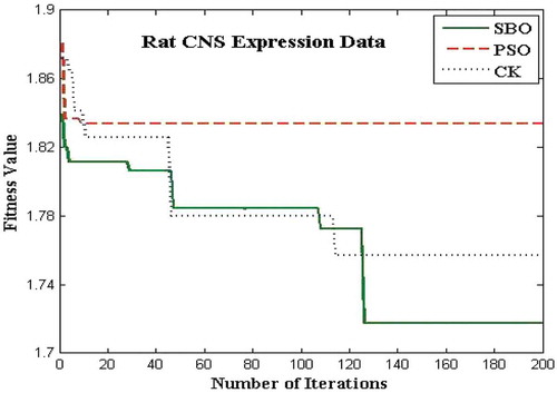
The proposed algorithms for the bicluster problems are coded in MATLAB and run on an Intel i3 3.7 GHz. The biclustering algorithm has been applied to four well-known datasets in order to study its performance: the yeast Saccharomyces cerevisiae stress expression data (Gasch et al. 2000), Arabidopsis thaliana expression data (Bleuler, Prelic, and Zitzler 2004), yeast Saccharomyces cerevisiae cell cycle expression data (Cho et al. 1998), and rat CNS expression data (Wen et al. 1998). The first Gasch yeast is the Saccharomyces cerevisiae with 2993 genes and 173 conditions. The second one, Arabidopsis thaliana expression data, contain 734 genes and 69 conditions. The third dataset, yeast Saccharomyces cerevisiae cell cycle expression, contains 2884 genes and 17 experimental conditions. The rat CNS dataset has a set of 112 genes under 9 conditions. Through empirical analysis, the population size and the number of iterations are set as 20 and 200 respectively. Figures 9–12 show the fitness value obtained for Saccharomyces cerevisiae expression data, Arabidopsis thaliana expression data, yeast Saccharomyces cerevisiae cell cycle expression data, and rat CNS expression data, respectively. The PSO has premature convergence due to stagnation. For all the datasets, the proposed SBO outperforms the PSO and CK algorithms because intensification and diversification is involved with the SBO algorithm.

FIGURE 9 Plot of number of iterations versus fitness value for yeast stress data.

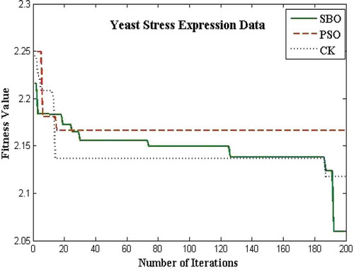
FIGURE 10 Plot of number of iterations versus fitness value for Arabidopsis thaliana data.

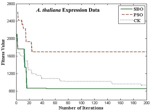
FIGURE 11 Plot of number of iterations versus fitness value for yeast cell cycle data.

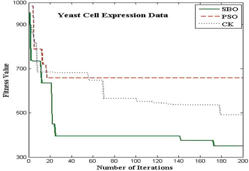
FIGURE 12 Plot of number of iterations versus fitness value for rat CNS data.

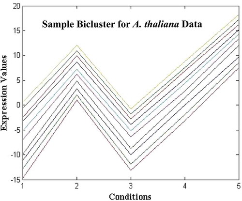
According to the problem formulation, the size of an extracted bicluster should be as large as possible while satisfying a homogeneity criterion. The bicluster should satisfy two requirements simultaneously. The expression levels of each gene within the bicluster should be similar over the range of conditions. That is, it should have a low MSR score. However, the bicluster gene variance should be high. The MSR represents the variance of the selected genes and conditions with respect to the homogeneity of the bicluster, and gene variance removes the simple (trivial) bicluster. In order to quantify the bicluster’s homogeneity and size, the Coherence Index (CI) is used as a measure for evaluating their goodness. CI is defined as the ratio of MSR score to the size of the formed bicluster. Tables 7–10 show sample experimental results obtained for Saccharomyces cerevisiae expression data, Arabidopsis thaliana expression data, yeast Saccharomyces cerevisiae cell cycle expression data, and rat CNS expression data, respectively, and the biclusters are chosen randomly from 20 biclusters. Clearly, Figure 13 shows a sample bicluster of size 10 × 5 for Arabidopsis thaliana data.

TABLE 7 Experiment Results for Saccharomyces cerevisiae Stress Expression Data

Bicluster No.	Genes	Samples	Volume	MSR	Gene Variance	CI	Fitness
BC1	1500	86	129000	0.6853	0.7049	5.3×10^−6	2.1039
BC3	1531	66	101046	0.7054	0.7226	6.9×110^−6	2.0892
BC7	1484	77	114268	0.7274	0.7505	6.4×10^−6	2.0598
BC10	1490	79	117710	0.6743	0.6914	5.7×10^−6	2.1206
BC15	1482	80	118560	0.6561	0.6773	5.5×10^−6	2.1325

TABLE 8 Experiment Results for Arabidopsis thaliana Expression Data

Bicluster No.	Genes	Samples	Volume	MSR	Gene Variance	CI	Fitness
BC1	366	26	9516	926.65	929.15	0.0973	926.65
BC2	353	29	10237	867.40	870.45	0.0847	867.40
BC6	364	25	9100	948.93	951.72	0.1042	948.93
BC9	377	32	12064	974.26	976.88	0.0807	974.26
BC17	347	35	12145	854.75	857.08	0.0703	854.76

TABLE 9 Experiment Results for Saccharomyces cerevisiae Cell Expression Data

Bicluster No.	Genes	Samples	Volume	MSR	Gene Variance	CI	Fitness
BC1	1422	3	4266	429.11	453.67	0.1005	429.12
BC3	1441	4	5764	464.19	499.22	0.0805	464.19
BC5	1440	2	2884	395.66	436.98	0.0934	395.66
BC7	1503	3	4509	534.79	553.01	0.1186	534.79
BC9	1404	6	8424	572.45	605.87	0.0679	572.46

TABLE 10 Experiment Results for Rat CNS Expression Data

Bicluster No.	Genes	Samples	Volume	MSR	Gene Variance	CI	Fitness
BC1	55	2	110	0.6169	0.9084	0.0056	1.7177
BC4	57	3	171	0.8038	1.0443	0.0047	1.7615
BC8	49	2	98	0.8797	1.1528	0.0089	1.7472
BC10	54	5	270	0.7881	1.0536	0.0029	1.7372
BC13	50	4	200	0.9190	1.2242	0.0045	1.7359

FIGURE 13 Plot of sample biclusters of size 10 × 5 for Arabidopsis thaliana expression data.

BIOLOGICAL ANALYSIS OF BICLUSTERS

Once high-level analysis methods have recommended some underlying structure in the data, then the results need to be interpreted and validated in terms of biological significance. The proposed work determines the biological relevance of the biclusters found by SBO on the Gasch yeast dataset in terms of the statistically significant Gene Ontology (GO) Annotation Database. In this database, the gene products are described in terms of associated biological process, components, and molecular functions in a species-independent manner. The degree of enrichment is measured by p-values, which use a cumulative hypergeometric distribution to compute the probability of observing the number of genes from a particular GO category (function, process, and component) within each bicluster. A bicluster is said to be over represented in a functional category if the p-value is below a certain threshold. The probability p for finding at least k genes from a particular category within a bicluster B of size m is given in Equation (16).

(16)

where G and r are the number of genes associated with the given category in the gene expression matrix and in the bicluster, respectively, while M and m are the number of genes in the gene expression matrix and in the biclusters, respectively. The p-value is the probability that the genes are selected into the cluster by random. If the p-value is smaller, then the match will be better. The annotations of genes for three ontologies including biological process, cellular component, and molecular function are obtained.

Biological Annotation for Yeast Stress Data Using GOTermFinder Toolbox

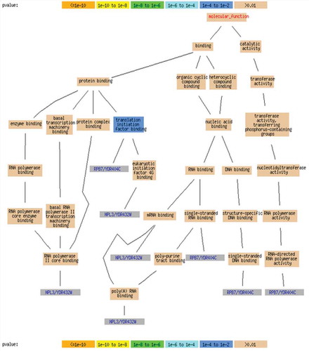
In order to identify the biological annotations for the biclusters, we use GOTermFinder,¹ which is a tool available in the Saccharomyces Genome Database. GOTermFinder is designed to search for the significant shared GO terms of the groups of genes and provides users with the means to identify the characteristics that the genes might have in common. Table 11 lists the significant shared GO terms used to describe the set of genes in each bicluster for the process, function, and component ontologies. Only the most significant terms are shown. For example, to the bicluster BC₁, the genes are mainly involved in binding activity. The tuple (n = 490, p = 7.82 × 10⁻⁸) represents that out of 1500 genes in bicluster BC₁, 490 genes belong to binding activity function, and the statistical significance is given by the p-value of p = 7.82 × 10⁻⁸. In Figure 14, the biological network of the bicluster with 10 genes, it is clear that the false discovery rate (FDR) is very low and it is zero on many occasions. Further, the corresponding p-value is very small (p = 0.000562), which shows that there is a very low probability to obtain the gene cluster in random. These results mean that the proposed SBO biclustering approach can find biologically meaningful biclusters.

TABLE 11 Significant GO Terms for Three Biclusters on Yeast Stress Data

Bicluster No.	No. of Genes	Process	Function	Component
BC1	1500	Cellular process	DNA binding activity	Intracellular part
		(n = 1386, p = 2.38×10^−144)	(n = 490, p = 7.82×10^−8)	(n = 1370, p = 2.90×10^−83)
BC3	1531	Single-organism process	Hydrolase activity	Cell part
		(n = 10836, p = 8.35×10^−91)	(n = 290, p = 2.06×10^−16)	(n = 1455, p = 1.07×10^−125)
BC7	1484	Metabolic process	Protein binding	Organelle
		(n = 1155, p = 8.71×10^−98)	(n = 227, p = 1.51×10^−20)	(n = 1180, p = 1.51×10^−64)

FIGURE 14 Gene ontology biological process of yeast stress data with 10 genes.

Functional Annotation for Arabidopsis thaliana Using DAVID Toolbox

The Functional Annotation Tool of the Database for Annotation, Visualization, and Integrated Discovery² is used for the enrichment analysis of the gene terms annotated for the input gene set. The basic principle behind the enrichment analysis is that, if a biological process is active/abnormal then the cofunctioning genes have a higher chance of being selected as a relevant group. Table 12 lists the significant GO terms used to describe the set of genes in each bicluster for biological activities. For example, for bicluster BC1 in Arabidopsis thaliana data, the GO process (GO: 0044271) is involved mainly in the nitrogen compound biosynthetic process. In this first row, 87 out of 366 genes belong to the nitrogen compound biosynthetic process; the total enrichment score is 44.61 and the statistical significance is given by the p-value of p = 9.5×10−52. The lower the p-value and the higher the gene enrichment value are, the more statically significant the bicluster is.

TABLE 12 Functional Annotation for Bicluster on Arabidopsis thaliana Data

GO Number	Ontology Description	Enrichment Score	Genes	p-value
GO:0044271	Nitrogen compound biosynthetic	44.61	87	9.5×10^−52
GO:0016053	Organic acid biosynthetic	44.61	83	3.1×10^−55
GO:0009536	Plastid	33.92	141	1.7×10^−22
GO:0009507	Chloroplast	33.92	139	2.5×10^−22
GO:0005996	Monosaccharide metabolic	14.86	42	3.6×10^−29

CONCLUSIONS

In this work, a novel algorithm, stellar-mass black hole optimization (SBO), is proposed for biclustering gene expression data. This optimization algorithm is deduced from the properties of a stellar-mass black hole. It is a nature-inspired, swarm-based, heuristic approach. Initially it starts with a random population of black holes and it endures to find the optimum mass of the universe. The mass of the black hole changes based on its absorption and emission. New solutions are generated by adjusting absorption and emission rates. When the mass of the black hole is small, it radiates more and finally it ends. When two black holes are in close proximity, they collide with each other. These properties are mimicked in the SBO algorithm to solve the optimization problems. SBO uses only a few parameters for adjusting. It contains both intensification and diversification during stagnation of the best solution. The results obtained from SBO are analyzed and compared with the swarm intelligence techniques PSO and CK with ten widely used benchmark optimization test functions and four benchmark gene expression datasets. The experiment results show that the proposed SBO outperforms the swarm intelligence techniques PSO and CK.

FUNDING

This work is supported by the research grant from Department of Biotechnology (DBT), Government of India, New Delhi, Grant No. BT/PR3741/BID/382/2011.

Additional information

Funding

This work is supported by the research grant from Department of Biotechnology (DBT), Government of India, New Delhi, Grant No. BT/PR3741/BID/382/2011.

Notes

¹ GOTermFinder for yeast stress data, http://www.yeastgenome.org/cgi-bin/GO/goTermFinder.pl.

² http://david.abcc.ncifcrf.gov/summary.jsp.

REFERENCES

- Androulakis, I. P., E. Yang, and R. R. Almon. 2007. Analysis of time-series gene expression data: Methods, challenges, and opportunities. Annual Review of Biomedical Engineering 9(2):205–228.
- Ayadi, W., M. Elloumi, and J. Hao. 2012. Pattern-driven neighborhood search for biclustering microarray data. BMC Bioinformatics 13(7): S11.
- Ayadi, W., and J. K. Hao. 2014 A memetic algorithm for discovering negative correlation biclusters of dna microarray data. Neurocomputing 145:14–22.
- Ben-Dor, A., B. Chor, R. Karp, and Z. Yakhini. 2003. Discovering local structure in gene expression data: The order-preserving submatrix problem. Journal of Computational Biology 10(4):373–384.
- Bergmann, S., J. Ihmels, and N. Barkai. 2003. Iterative signature algorithm for the analysis of large-scale gene expression data. Physical Review E 67:1–18.
- Bleuler, S., A. Prelic, and E. Zitzler. 2004. An EA framework for biclustering of gene expression data. In Proceedings of the congress of IEEE on evolutionary computation 166–173. IEEE.
- Chaisson, E., and S. McMillan. 2008. Astronomy today: Stars and galaxies (5th ed,). UK: Benjamin Cummings/Pearson.
- Cheng, Y., and G. M. Church. 2000. Biclustering of expression data. In Proceedings of the 8th international conference on intelligent systems for molecular biology 8:93–103. San Diego, CA, USA: AAAI Press.
- Cho, R. J., M. J. Campbell, E. A. Winzeler, L. Steinmetz, A. Conway, L. Wodicka, T. G. Wolfsberg, A. E. Gabrielian, D. Landsman, and D. J. Lockhart. 1998. A genome-wide transcriptional analysis of the mitotic cell cycle. Molecular Cell 2:65–73.
- Civicioglu, P., and E. Besdok. 2011. A conceptual comparison of the cuckoo-search, particle swarm optimization, differential evolution and artificial bee colony algorithms. Artificial Intelligence Review doi:10.1007/s10462-011-9276-0.
- Coelho, G. P., F. O. de Franca, and F. J. V. Zuben. 2009. Multi-objective biclustering: When non-dominated solutions are not enough. Journal of Mathematical Modelling and Algorithms 8(2):175–202.
- DiMaggio, P., S. McAllister, C. Floudas, X. Feng, J. Rabinowitz, and H. Rabitz. 2008. Biclustering via optimal re-ordering of data matrices in systems biology: Rigorous methods and comparative studies. BMC Bioinformatics 9(1):458–467.
- Divina, F., and J. S. Aguilar-Ruiz. 2006. Biclustering of expression data with evolutionary computation. IEEE Transactions on Knowledge Data Engineering 18(5):590–602.
- Gasch, A. P., P. T. Spellman, C. M. Kao, O. Carmel-Harel, M. B. Eisen, G. Storz, D. Botstein, and P. O. Brown. 2000. Genomic expression programs in the response of yeast cells to environmental changes. Molecular Biology of the Cell 11:4241–4257.
- Gottesman, D. 1997. Stabilizer codes and quantum error correction. quant-ph/9705052 (PhD thesis, California Institute of Technology, Pasadena, CA, USA).
- Hamilton, A. J. S. 1998. The evolving universe. Dordrecht, The Netherlands: Kluwer Academic.
- Hartigan, J. A. 1972. Direct clustering of a data matrix. Journal of the American Statistical Association 67(337):123–129.
- Huang, Q., D. Tao, X. Li, and A.W.C. Liew. 2012. Parallelized evolutionary learning for detection of biclusters in gene expression data. IEEE/ACM Transactions on Computational Biology and Bioinformatics 9(1):560–570.
- Jaccard, P. 1912. The distribution of the flora in the alpine zone. New Phytologist 11(2):37–50.
- Karaboga, D., and B. Akay. 2009. A comparative study of artificial bee colony algorithm. Applied Mathematics and Computation 214(12):108–132
- Liu, C. L. 1968. Introduction to combinatorial mathematics. New York, NY: McGraw-Hill.
- Liu, J., Z. Li, X. Hu, and Y. Chen. 2009. Biclustering of microarray data with mospo based on crowding distance. BMC Bioinformatics 10(4):S9.
- Liu, X., and L. Wang. 2007. Computing the maximum similarity bi-clusters of gene expression data. BMC Bioinformatics 23(1):50–56.
- Lockhart, D. J., and E. A. Winzeler. 2000. Genomics, gene expression and DNA arrays. Nature 405:827–836.
- Luminet, J. P. 1998. Black holes: A general introduction. In Black holes: Theory and observation, Lecture Notes in Physics 514:3–34. Berlin, Heidelberg: Springer-Verlag.
- Maatouk, O., W. Ayadi, H. Bouziri, and B. Duval. 2014. Evolutionary algorithm based on new crossover for the biclustering of gene expression data. In Pattern Recognition in Bioinformatics, LNCS 8626:48–59. Switzerland: Springer International.
- Madeira, S. C., and A. L. Oliveira. 2004. Biclustering algorithms for biological data analysis: A survey. IEEE/ACM Transactions on Computational Biology and Bioinformatics 1(1):24–45.
- Mitra, S., and H. Banka. 2006. Multi-objective evolutionary biclustering of gene expression data. Pattern Recognition 39(12):2464–2477.
- Mukhopadhyay, A., U. Maulik, and S. Bandyopadhyay. 2010. On biclustering of gene expression data. Current Bioinformatics. 5:204–216.
- Murali, T., and S. Kasif. 2003. Extracting conserved gene expression motifs from gene expression data. Pacific Symposium on Biocomputing 8:77–88.
- Roy, S., D. K. Bhattacharyya, and J. K. Kalita. 2013. CoBi: Pattern based co-regulated biclustering of gene expression data. Pattern Recognition 34(14):1669–1678.
- Tanay, A., R. Sharan, and R. Shamir. 2002. Discovering statistically significant biclusters in gene expression data. BMC Bioinformatics 18:136–144.
- Tasgetiren, M. F., and Y. C. Liang. 2007. A binary particle swarm optimization algorithm for lot sizing problem. Journal of Economic and Social Research 5(2):1–20.
- Wen, X., S. Fuhrman, G. S. Michaels, D. B. Carr, S. Smith, J. L. Barker, and R. Somogyi. 1998. Large-scale temporal gene expression mapping of central nervous system development. Proceedings of the National Academy of Sciences 95(1):334–339.
- Yang, X. S., and S. Deb. 2009. Cuckoo search via Levy flights. In Proceedings of the IEEE world congress on nature & biologically inspired computing 210–214. IEEE Publications.