A Randomized Algorithm for the Exact Solution of Transductive Support Vector Machines

Abstract

Random sampling is an efficient method for dealing with constrained optimization problems. In computational geometry, this method has been successfully applied, through Clarkson’s algorithm (Clarkson 1996), to solve a general class of problems called violator spaces. In machine learning, Transductive Support Vector Machines (TSVM) is a learning method used when only a small fraction of labeled data is available, which implies solving a nonconvex optimization problem. Several approximation methods have been proposed to solve it, but they usually find suboptimal solutions. However, a global optimal solution may be obtained by using exact techniques, but at the cost of suffering an exponential time complexity with respect to the number of instances. In this article, an interpretation of TSVM in terms of violator space is given. A randomized method is presented that extends the use of exact methods, thus reducing the time complexity exponentially w.r.t. the number of support vectors of the optimal solution instead of exponentially w.r.t. the number of instances.

INTRODUCTION

In computational geometry, random sampling is an efficient method for dealing with constrained optimization problems. First, one finds the optimal solution subject to a random subset of constraints. Likely, the expected number of constraints violating that solution is significantly smaller than the overall number of remaining constraints. Even in some lucky cases, the found solution does not violate the remaining constraints. Hence, one can exploit this property to build a simple randomized algorithm. Clarkson’s algorithm (Clarkson 1996) is a two-staged random sampling technique able to solve linear programming problems, which can also be applied to the more general framework of violator spaces. The violator space framework has become a well-established tool in the field of geometric optimization, developing subexponential algorithms starting from a randomized variant of the simplex method. The class of violator space includes the problem of computing the minimum-volume ball or ellipsoid enclosing a given point set in R^d, the problem of finding the distance of two convex polytopes in R^d, and many other computational geometry problems (Gartner, Matousek, and Skovron 2008). Generalization of violator space problems makes them applicable to a number of nonlinear and mostly geometric problems. Clarkson’s algorithm stages are based on random sampling and are conceptually very simple. Once it is shown that a particular optimization problem can be regarded as violator space problem, and certain algorithmic primitives are implemented for it, Clarkson’s algorithm is immediately applicable.

In machine learning, Transductive Support Vector Machine (TSVM; Vapnik 1995) extends the well-known Support Vector Machines (SVM) to handle partially labeled datasets. TSVM learns the maximum margin hyperplane classifier using labeled training data that does not present unlabeled data inside its margin. Unfortunately, dealing with a TSVM implies solving a nonconvex optimization problem. A wide spectrum of approximative techniques have been applied to solve the TSVM problem (Chapelle 2008), but they do not guarantee finding the optimal global solution. In fact, when state-of-the-art approximative TSVM methods have been applied to different benchmark problems, far from optimal solutions have been found (Chapelle 2008). Unfortunately, exact methods can be applied only to small datasets because of the exponential time complexity cost with respect to the number of instances. Balcazar et al. (2008) suggested that a hard-margin SVM belongs to the class of violator space, proposing a random sampling technique for the determination of the maximum margin separating hyperplane. Note that the problem of solving an SVM is convex, whereas solving a TSVM is a non-convex problem, so they are very different in nature. In this article we prove that the global optimal solution of a TSVM totally relies on the knowledge of the support vectors set, gathering a size smaller than the whole set of instances. Moreover, we also demonstrate that TSVM can be formulated as a violator space problem, allowing the use of the Clarkson’s algorithm to find its optimal global solution. Fostering the TSVM sparsity property, we introduce a randomized algorithm able to reduce the time complexity of exact methods, scaling, thus, exponentially w.r.t. the number of support vectors of the optimal solution instead of exponentially w.r.t. the number of instances. Using our method, one may find the exact solution independently of the number of instances when the problem has few support vectors. This includes problems for which the dimensionality in the feature space is relatively small.

VIOLATOR SPACES AND RANDOMIZED ALGORITHMS

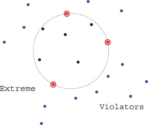
Violator space problems were introduced as an abstract framework for randomized algorithms able to solve linear programs by a variant of the simplex algorithm. In computational geometry, an example problem that can be solved using this method is the smallest enclosing ball (SEB). Here the goal is to compute the smallest ball enclosing a set of n points in a d dimensional space (Figure 1). In the following we introduce the main tools of the abstract framework of violator spaces in order to show how randomized methods devised in computational geometry can also be applied to solve the TSVM problem. Details and proofs of the reported properties can be found in Gartner et al. (2008).

FIGURE 1 Smallest enclosing ball: extremes (red circled in red) are the points essential for the solution, violators (in blue) are the points lying outside the ball, a basis is a minimal set of points having the same ball.

Definition 2.1

An abstract LP-type problem consists of a finite set H, representing the constraints of the problem, a weight function w giving for the cost of the optimum solution, W linearly ordered . satisfy:

• Monotonicity: for all , we have and

• Locality: for all and all with and , we have .

For a , a basis is an inclusion-minimal subset such that . The combinatorial dimension of an LP-type problem is the size of the largest basis. A violator of G is an additional constraint such that . An element h is an extreme of G if . From the definition, h violates is extreme in . The set of all constraints violating G is called a violator mapping

Using the violator mapping, it is possible to phrase the LP-type problem in terms of violation tests, neglecting the explicit evaluation of w:

Definition 2.2

A violator space is a pair (H, V) with H a finite set and V a mapping. (H, V) satisfy:

• Consistency: holds for all and

• Locality: for all where we have .

Given an LP-type problem (H, w, W, ), the pair (H, V) is a violator space, which is the most general framework applying to the randomized algorithm described later. In a violator space (H, V) of combinatorial dimension , in order to set up a basis evaluation algorithm, we need to define the following primitive operation:

Primitive 2.3

(Violation test) (H, V) violator space can be implicitly defined by the primitive: given and decide whether

Consider a suitable violator space and define

as the set of violators of R while

is the set of extremes of R. The following result holds:

Lemma 2.4

(Sampling Lemma) For a set R of size r, uniformly chosen at random from the set of all r-element subsets of G with , define two random variables with expected values , . Now, for we have .

Therefore, in a violator space with and combinatorial dimension choosing a subset R, the sampling lemma bounds the expected number of violators through .

Clarkson (1996) envisaged a smart randomized algorithm able to solve violator space problems relying on the expected number of violators bounded according to the sampling lemma. In the SEB case, w is represented by the radius of the ball, H is the set of constraints requiring all the points inside the ball, violators are points outside the ball. It can be proved that SEB is a violator space problem and Clarkson’s algorithm can be used to solve it. The algorithm proceeds in rounds, maintaining a voting box that initially contains one voting slip per point. In each round, a set R of r voting slips is drawn at random without repetitions from the voting box and the SEB of the corresponding set R is computed. For each new round, the number of voting slips for the violators points is doubled. The algorithm terminates as soon as there are no violators (no points outside the ball). If , the expected number of rounds is O(log n), reducing a problem of size n to O(log n) problems of size O.

In the Clarkson’s algorithm, the problem of finding a basis is solved by using a trivial algorithm able to find the solution for subsets of size at most . Clarkson’s Basis2 algorithm calls the trivial algorithm as a subroutine, increasing the probability of obtaining a base in further iterations. Consider G as a multiset with μ(h) (initially set to one) denoting the multiplicity of h. For a set , the compound multiplicity of all elements of F is . Sampling from G is done envisaging that it contains copies of every element h. At each round, when the number of violators is below a threshold, Basis2 doubles the multiplicity μ (weight) of violator points, which increments the probability of selecting a base in next rounds. Convergence of the Basis2 algorithm relies on the fact that the trivial algorithm is correct. An iteration of the loop is successful if it changes the weights of the elements. To estimate how many unsuccessful iterations pass between two successful ones, the sampling lemma bound can be used. Hence, it can be shown that after k successful iterations

holds for every basis B of G with and in particular . Summarizing Clarkson’s algorithm: Basis2 computes a basis of G with an expected number of at most calls to primitive 1, and an expected number of at most calls to the trivial with sets of size .

TRANSDUCTIVE SUPPORT VECTOR MACHINES

TSVM can be described as a training set of l labeled examples where with labels and i.i.d. according to an unknown distribution p(x, y) together with u unlabeled examples with and the total number of examples, distributed according to some distribution p(x). Considering w to be the vector normal to the hyperplane and the constant b, the problem can be formulated as finding the vector of labels having the maximal geometric margin with a separating hyperplane (w, b), solving

(1)

with or 2, respectively, for linear (L₁) losses and quadratic (L₂) losses. The first term controls the generalization capacity whereas the others, through the slack variables , control the number of misclassified samples. The two regularization parameters (C and C*) should justify our confidence in the known labels. The decision function in the hypothesis space is represented as

and assuming there exists a given Hilbert space and a mapping . The mapping sends the examples data into a feature space, generating the kernel and satisfying the Mercer’s conditions. In this work we refer to quadratic losses, because once the is fixed, the associated Hessian matrix is positive definite, making an objective function unique and strictly convex. Moreover, the optimization problem is considered computationally more stable for L₂ losses. However, main results still apply for the L₁ losses case. Early on, two main strategies were adopted to minimize :

• local approximation methods: starting from a tentative labeling , they perform a local search in the space of labelings, using effective heuristics, to maximize . These methods are sensible to local minima. For instance, SVM^light method (Joachims 1999) uses a local search algorithm to find the solution, which may fail in delivering a solution close to the global one.

• exact combinatorial methods: fixing the unlabeled vector in converts the optimization over (w, b) into a standard SVM. Combinatorial methods find the global optimal solution by searching on the entire space of possible labelings of for the SVM with maximum margin.

Focusing on exact combinatoria optimization of , the objective becomes to minimize over a set of binary variables. Such an optimization is nonconvex, belonging to the computational class of NP-hard. It can be solved, for instance, by using branch and bound (BB; Chapelle, Sindhwani, and Keerthi 2006) or integer programming (IP; Bennett and Demiriz 1998), but they are computationally very demanding because of the large number of different possible labelings of unlabeled instances.

Critical Analysis of TSVM Exact Global Solution

An examination of the optimization problem shows that the optimal solution does not depend on the labeling of all unlabeled data, but on the labeling of the support vectors of the optimal solution because of the sparsity property of SVMs.

Observation 3.1

Assume having a set of labeled and a set of unlabeled examples. Name the vector of labels solving the TSVM with cost (i.e., the labeling of instances with lower cost). Now consider to be the inductive SVM with labels . Then, adding an unlabeled point x to the set , lying outside the margin of , induce the optimal labeling for the transduction problem on to be (y_x being the label induced by on x).

Proof

Assume the existence of a different labeling better than , such that leads to a contradiction. Consequently, must be the optimal labeling. In fact, from the assumption, we have , but because adding a point x lying outside the margin of does not change the SVM solution, it follows that . Finally, stems because adding one point to a given labeling can only increase or leave unchanged its cost. Therefore, and, consequently, is a contradiction, due to the hypothesis that represents the optimal labeling for set .□

Observation 3.2

Assume having a set of labeled and a set of unlabeled examples. Consider a subset with a given vector of labels y_R solving the TSVM for the set and let be the inductive SVM with labels . Assume we don’t have points in lying inside the margin of . In this case, the optimal labeling for the TSVM on is represented by , being the vector of labels induced by the solution of , on the set .

Proof

This can be proved by applying Observation 3.1 for any point in . Starting with label vector , and noticing that any point in lies outside the margin of , then iteratively applying the Observation 3.1, we end up with the global solution for .□

Observation 3.3

Necessary condition to find the global optimal solution for the set of points using the subset is that must contains all support vectors of the global optimal solution in

Proof

This can be proved by applying Observation 3.2. Note that the optimal solution for can be built from . The only condition is that points in do not lie inside the margin. Henceforth, there won’t be support vectors in , all of them being in .□

According to these observations, we may come to the following conclusion: Given a TSVM, most of data points may be unnecessary for building the global optimal solution. The set of support vectors completely defines the global optimal solution (TSVM sparsity property). This suggests that it can be feasible to obtain the TSVM optimal global solution when the set includes the whole set of support vectors. Therefore, the question becomes how to get the right subset of points. We claim that the TSVM solution may be obtained working on a reduced subset of examples with computational leverages when . Noticeably, for a TSVM, we may show how to build a violator space solving the problem by using randomized algorithms. It is worth noting that this method might be of practical use whenever the number of support vectors in the solution of the TSVM problem scales with O(log n), which is not usually the case. However, the method can still be applied when the solution has few support vectors or when the dimension of the feature space of the problem is relatively small.

RANDOMIZED ALGORITHMS FOR TSVM

In this section we are ready to show that a TSVM problem belongs to the class of violator space. Therefore, Clarkson’s algorithm can be used to find its optimal global solution. In this case, the weighting function w is represented by evaluated over subset of constraints with combinatorial dimension depending on the number of support vectors. Given a subset of partially labeled points, TSVM global optimal solution (a basis) can be obtained using an exact method such as IP or BB (our trivial algorithm). Moreover, we need to define a violation test because Clarkson’s algorithm relies on the probability of selecting a basis increasing the weight of violating points. Then, we will show that violators can be easily detected as the remaining points lying in the TSVM separating margin. TSVM may also arouse a formulation in terms of violator space problem. Endowing the constrained formulation of the TSVM problem and violator space definition we formally propose:

Proposition 4.1

Given a TSVM with constraints , , a mapping defined for each subset as , , and bounded and linearly ordered by , the quadruple represents an associated violator space problem.

In order to verify locality and monotonicity we need to prove the lemma:

Lemma 4.2

Given a TSVM with constraints and a subset with global optimum , adding a constraint to will change the global optimum according to .

Proof

The lemma may be easily proven by contradiction. Suppose the lemma is not true; then . Now, the solution to the TSVM problem on the set of constraints is also a feasible solution for the TSVM problem on the set of constraints . Hence, the hypothesis contradicts the minimality of the TSVM solution . However, because we need to provide the primitive in order to build the violator space, we need a more constructive proof of the lemma following the incremental solution of the TSVM. Therefore, consider the subset of constraints ; getting the objective means to find the global optimal solution of the TSVM problem using a subset of labeled and unlabeled data . With an exact method, the quest for the global optimum over the subset of constraints entails that among the possible configurations of vector of labels , we cast the corresponding SVM with minimum objective , which, solving the dual problem, can be written as . Adding another constraint with vector of labels means that among possible configurations, we select the corresponding SVM with minimum objective , which, solving the dual problem, can be expressed as . Hence, the relationship between the two objective values can be found, considering the incremental training analysis of an SVM as reported in (Cauvemberghs and Poggio 2001), with some differences in our case gathered from quadratic losses.

The SVM dual problem might be obtained by introducing , the Lagrangian multipliers, and considering that for the optimal solution the KKT conditions must be satisfied. After elimination of w, (note that for quadratic losses if , then ), we get the dual problem

(where or , accordingly), and defining

( if , 0 otherwise), the KKT conditions for the support vectors are and , which, defining the vectors Y and α, can be equivalently expressed in a more compact form as

(2)

The KKT for nonsupport vectors can be expressed as . Finally, the solution of the dual problem gives the maximum value of the , which, substituting the KKT conditions and defining

can be written as . In incremental training, adding a new point h consists adiabatically incrementing starting from and changing the other parameters until the KKT conditions for point h are fulfilled. The increment of is done ensuring that the KKT conditions for the other points are maintained. In the following, is defined as the difference between the new alpha value ’ and the old value . The KKT conditions before and after the update connect the variations of the support vectors , , and the added according to:

For support vectors , then

(3)

gathering

Tackling those equations, we may infer the change due to the presence of a new datum as a function of the . Unfortunately, with a generic value , we cannot directly use these systems to obtain the new state, due to the possible change of composition in the sets of support vectors and nonsupport vectors while increases. Handling this situation demands a bookkeeping of possible adiabatic modifications. So, the procedure consists in incrementing to the maximum until one of the following cases arise: the problem is solved, or the keeping of the KKT conditions of the other points forces us to change the set of support vectors.¹ In particular, dealing with the increment of might make changes in the support vectors composition depending on the amount of . Here, we detail the possible situations:

• and , the new point with the chosen label won’t change the set of support vectors and we keep the same solution

• and (g value after the increment of ), the new point with the chosen label is a new support vector, while the support vector set does not change composition (no migrations), hence, the new KKT can be written as

  ensuing a connection with the old solution across the Sherman–Morison–Woodbury formula for block matrix inversion:
  with
  (4)
  where due to a semidefinite positive kernel wherefrom we can express the updated values
  and
  using with optimum update
  which entails .

• and , the new point with the chosen label y_h is a new support vector while the support vectors set changes composition. For quadratic losses, this means two possibilities: whether one support vector, say it is k with and , becomes a nonsupport vector, hence and or vice versa (from and to and ). In each of these cases, the condition holds. As the set of support vectors does not change during increment (it changes after the increment), the global optimum after and before each increment accordingly may be evaluated as:

  where and , allowing us to evaluate the global optimum increment as

  Now, using Equation (3) to express the change in the global optimum as a function of , it can be written as:

  and

  One can easily show that

  because is negative (see assumptions of this case) and q_h is always positive.

We have assumed that the set of equations describing the evolution of the α_i for all points does not change during each step. However, while increasing the , we have to check if the KKT conditions are still verified. Consequently, if such conditions are no longer fulfilled for a given point, this status has to change (from support to nonsupport vector or vice versa, depending on the case) and, therefore, the equations must be modified according to the bookkeeping. Finally, it remains to be seen if the objective function is still monotonous when we change the equations and the support vector set. It is easy to see that for the L₂ losses, the bookkeeping does not change the value of the objective function. In fact, bookkeeping is necessary when one support vector becomes a nonsupport vector or the other way round. In both cases, the α_k of the point changing its status is 0 (if the point is a new support vector, its α_k will increase up from 0; or, if it leaves the status of support vector, its alpha value will decrease to 0). When , adding or removing it does not modify the objective function. Consequently, the objective function does not change by doing bookkeeping.

We conclude that for an incremental SVM, the optimum grows monotonically. Henceforth, using an exact method to solve the TSVM over means that we look for the global optimal solution among the 2^r SVMs, corresponding to the possible labelings , while over we look for the global optimal solution among the SVMs, corresponding to the possible labelings . Then, we may realize that the labeling for the global optimum over , except for the new constraint , may be different from the labeling corresponding to the global optimum over . Therefore, thanks to the fact that the SVM global optimal solution monotonically increases when moving from to and that the global optimal solution for an exact method seeks for the minimum among all the possible SVMs, it follows that .□

The previous lemma, which provided monotonicity of the incremental optimal solution for a TSVM, allows us to infer that represents a violator space (from LP-type) problem, and we report here the proof for the Proposition 4.1.

Proof

We need to show only that monotonicity and locality hold:

• Monotonicity: Given the subsets of constraints and such that , we can always build from through an incremental process adding new constraint . From Lemma 4.2, it follows that .

• Locality: Given the subsets of constraints and such that and a constraint . If , the two sets entail the same global solution. Adding incrementally the constraint to the subset with conveys that the new constraint has changed the global solution. Consequently, adding to will also change the global solution, then, .□

Facing our definition of the associated violator space problem for a TSVM, a basis is represented by a set of the support vectors in the global solution, the cardinality of the largest one being the combinatorial dimension. At this stage we have shown that it is indeed feasible to formulate a TSVM as a violator space problem. In addition, adopting the Clarkson’s algorithm, we may also use the violator mapping through the violation test.

Primitive 4.3. (TSVM violation test)

Given a TSVM with global solution over subset of constraints and decision function , any other constraint will violate the solution (), if with the label obtained through .

Beforehand we have shown that we may associate a violator space problem to a TSVM once we deal with an exact method to get the optimal global solution. Remarkably, Clarkson’s randomized method is viable to solve a TSVM acquiring a basis using the violation test of Primitive 4.3. Efficiency relies on the sparsity property of TSVM.

ALGORITHM IMPLEMENTATION

Exact methods such as IP (Bennett and Demiriz 1998) and BB (Chapelle et al. 2006) have been investigated for TSVM. The basic idea of IP for TSVM is to add an integer decision variable indicating the class for each point in the working set. Hence, the solution can be found using any mixed integer programming code, provided that the computer resources are suitable for the size of the problem. BB is another method able to solve combinatorial optimization problems using an enumerative technique to implicitly and efficiently search into the entire space of solutions.

Algorithm 1

STSVM (X_l, Y_l, X_u, maxit, r)

Require:

repeat

 Choose X_r at random according to μ distribution:

 Base(obj_R, Y_r, α, w, b) := BB(X_l, X_r, Y_l) // call branch and bound

  // compute labels …

  // … and slacks

  // check violators

 if then

  , // update weights of violators

 end if

  // update best …

 Base_best := min_OBJ(Base(OBJ_R, Y_r, α, w, b), Base_best) // … known solution

until maxit or

if then

 return Base(obj_R, Y_r, α, w, b) // global optimum

else

 return Base_best // best solution found

end if

Clearly both methods, or even any other exact TSVM, could be used to implement the trivial algorithm. For practical reasons, in the following we focus only on BB implementation, indicating with BBTSVM the one devised by Chapelle for TSVM. It solves the problem over a set of binary variables where each evaluation of embodies an inductive SVM. BBTSVM minimizes over 2^u possible choices of y_u. At each node in the binary search tree, a partial labeling of the datasets is generated and for the corresponding ones casts the labeling of some unlabeled data. The core of the BBTSVM is a subroutine akin the primitive evaluation of an SVM on the data already labeled as we proceed in the search tree. SVM are usually solved as constrained quadratic programming problems, in the dual, but they can also be worked out in the primal as unconstrained. BBTSVM uses this method, requiring few iterations to get an approximate solution with a (worst case) complexity O(n³). SVMs, being convex quadratic program problems, are polynomial-time solvable, the currently best method raising (worst case) a complexity of O(n³/²d²). By the enumeration process, BBTSVM may reach a complexity from O(2ⁿn³) to O(2ⁿn³/²d²) depending on the SVM solver used.

Implementation of Randomized TSVM

Having set out the matter in this way, we are ready to encompass the details of our implementation of a randomized version for an exact method to solve TSVM, which we will refer as STSVM. The Algorithm (1) implementing the STSVM slightly revises Clarkson’s scheme. In general, we may ignore the combinatorial dimension of the corresponding violator space. In fact, apart from the linear case, theoretical bounds on the number of support vectors are not of practical use. Henceforth, we start with a fixed given value for r_o. According to Basis2, to stress the probability of selecting a given violator in further rounds, we double the corresponding weight whenever the slack . In the quadratic loss implementation, for example, where , it means that the point would change the margin if added to the basis. The basic implementation of the trivial algorithm makes use of an implementation of an exact method of working over random samples . As envisaged, in the practical implementation of the trivial algorithm, we will make use of BB. However, using a different exact algorithm to provide the implementation of the trivial does not change the convergence of STSVM but can only affect the performances. Two stop conditions are foreseen: (1) (no violators condition: returns global optimum) or (2) max number of iterations (returns best known solution). In the last case, the best known solution is represented by the minimum of , where , with the correction factor in the incremental update of the Equation (4). Such criterium takes into account obj_R the best result from BB, also minimizing the violators contribution . Our implementation of BB is able to optimize the undergoing SVM either in the primal or dual formulation with quadratic or linear losses.

Convergence and Complexity of STSVM

Applying the sampling lemma, the expected value E[V_Base] for elements in (with ) violating the random set R, (casting with ) can be bound as

Markov inequality predicts

implying that the expected number of rounds is at most twice as large as the number of successful ones. Let be the set of support vectors for the TSVM, at each successful iteration some won’t be in , hence, gets doubled. Since , it means some x_i gets doubled at least once every successful rounds and after k rounds . However, every successful round raises the total weight by at most

giving the bound

After kδ successful iterations, the lower bound exceeds the upper when . Finally, the expected number of violation tests is at most , whereas the expected number of calls to BBTSVM is at most , and sets R have average size (at most r_max).

Time complexity of STSVM shows that the sparsity property allows for a relative gain with respect to the use of a BB over the whole set of data from to . Our method is effective when the number of support vectors is much lower than the number of instances.

EXPERIMENTS

In this section we briefly describe results obtained using the proposed randomized method in two well-known benchmark problems that have not been previously solved using exact methods.

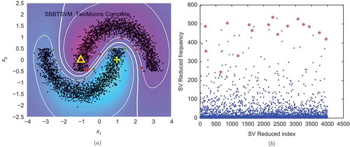
STSVM stands out on the well-known benchmark problem of two moons now composed of 4.000 unlabeled examples (Figure 2). The two moons problem has been reported burdensome to solve for state-of-the-art transduction methods (Chapelle 2008). Table 1 shows error rates produced by some of these methods in a small dataset containing 200 unlabeled points. All these methods fall in local minima very far from the global one. However, this problem has been solved previously by applying BB over the space of all possible labeling of instances (Chapelle et al. 2006). Unfortunately, albeit the method is able to find out the optimal solution, it has an exponential time complexity on the number of unlabeled instances, consequently, it is able to solve the two moons only for datasets up to a few hundreds of unlabeled instances. The method described in this article finds the optimal solution but instead of scaling with the number of instances, it scales with the number of support vectors. In the case of the two moons, the number of support vectors does not scale with the number of points. Henceforth, faced with 4.000 unlabeled examples through STSVM allows us to find the exact solution within a few minutes.

TABLE 1 Error rate on datasets for supervised SVM, state-of-the-art transduction algorithms (as reported in Chapelle 2008), and STSVM

datasets	SVM		cS^3VM	CCCP	S^3VM^light		Newton	STSVM
TwoMoons	50.2	61	37.7	63.1	68.8	22.5	11	0
Coil3	66.6	61.6	61	56.6	56.7	61.6	61.5	0
Coil20	24.1	25.6	30.7	26.6	25.3	12.3	24.1	1.4

FIGURE 2 (a) Distribution and exact solution for the two moons dataset (4.000 unlabeled, 2 labeled as triangle and cross). (b) Weights distribution for the whole set of points at the final round. Support vectors of the optimal solution are encircled.

STSVM is also able to find the exact solution for another well-known benchmark problem that has not been previously solved using exact methods: the Coil20 dataset (described in (Nene, Nayar, and Murase, 1996)). It contains 1440 images of 20 objects photographed with different perspectives (72 images per object) with 2 labeled images for each object. Coil20 belongs to multi-class problems commonly solved through a one-vs-all scheme. This scheme, builds a SVM for each class assigning labels according to the class returning a maximum output for a given point, which is a measure of confidence of classification for that point. Table 1 shows the success of state-of-the-art transduction algorithms on this dataset as described in Chapelle (2008). BBTSVM is not able to solve this problem, because of the large number of instances, albeit it can manage the Coil3 with pictures of solely 3 classes but it is difficult to discriminate. STSVM finds a solution with 0 error for Coil3 dataset while Table 1 illustrates the errors produced by state-of-the-art transduction methods (from Chapelle 2008). In the last two columns, the error rate of L₂ losses (used in the search tree of STSVM) applied only to the labeled examples are reported, as well as the results obtained by STSVM with the one-vs-all scheme acting over labeled and unlabeled. Remarkably, the difference between the baseline results shown in Chapelle (2008) and ours come from the different losses used for the SVM (L₂ in our case, L₁ for the others). Even though STSVM might be used with different losses, here we stress the error reduction (from to 10.9% in Coil20, and 0% in Coil3), more that its absolute value. However, examining the 20 TSVMs produced in the one-vs-all scheme (one for each class), it may be noticed that some TSVMs have not found 0 violators after 100 iterations or that when a solution with 0 violators was found, it did not show the right balance between positive and negative examples. On the other side, some TSVMs returned solutions with 0 violators and the right rate between positive and negative examples. We considered these TSVMs as good predictors for the classes they represent and kept them. The points labeled as positive for these classes were removed from the whole dataset, delivering a smaller one. Afterward, we tried to solve this smaller dataset by applying the one-vs-all scheme again on the remaining classes. As the problem has been simplified, now there appear new good predictors for some classes and the procedure is repeated until the whole dataset is completely solved. The final error following this procedure was 20 errors from the 1400 unlabeled initial examples, reducing the error for Coil20 to 1.4%. Quite remarkably, the irreducible errors were produced between classes 5 and 19, the last classes for which the method found a good predictor. It seems that for these 2 classes the maximum margin hypothesis does not hold and that some additional constraints must be used to correctly classify them; in fact, modifying the ratio only among labeled and unlabeled largely increases the former; this problem can be correctly solved.

CONCLUSIONS AND FUTURE WORK

In this article, we have shown an original interpretation of the TSVM problem in terms of violator space. Our version is able to extend the use of any exact method to find the optimal solution, but scales in time complexity with the number of support vectors instead of the number of points. The most suitable situation for our method applies to datasets entailing a small number of support vectors, independently of the size of the dataset. Limitations of our approach appear when the size of the support vectors set is higher than a few hundreds, a common situation in real datasets. In the future, we plan to investigate an implementation using very sparse SVMs formulations, which might allow extending the application of our method to larger datasets.

Also, preliminary experiments with larger benchmark datasets (where the number of support vectors were in the range of hundreds) show that the method is, as we expected, not able to find the optimal solution in a reasonable time. However, in these cases we kept the best solution, as described in “Implementation of Randomized TSVM.” In all cases, the returned solution was better than that returned by an SVM on only the labeled examples. These experiments encourage us to explore error bounds for the proposed methods and try to apply them to find good approximations to the optimal solution.

Finally, we consider interesting a possible interpretation of the weight obtained for each example in the randomized method. Samples with high weights usually appear as violators, which could help us identify points interesting for the final solution even if the method is not able to find the exact solution.

ORCID

G. Esposito

http://orcid.org/0000-0002-9700-2971

FUNDING

This work was partially supported by the FI-DGR programme of AGAUR ECO/1551/2012.

Additional information

Funding

This work was partially supported by the FI-DGR programme of AGAUR ECO/1551/2012.

Notes

¹ Note that in the case of quadratic losses we need to divide sets of points into only two sets: supports (S) and others (O), whereas, in the case of linear losses, points can belong to three different sets: supports (S), errors (E), and others (O).

REFERENCES

- Bennett, K., and A. Demiriz. 1998. Semi supervised support vector machines. In Advances in neural information processing systems (NIPS), 12:368–374. Cambridge, MA, USA: MIT Press.
- Cauvemberghs, G., and T. Poggio. 2001. Incremental and decremental support vector machine learning. In Advances in neural information processing systems (NIPS). 13:409–415. Cambridge, MA, USA: MIT Press.
- Chapelle, O. 2008. Optimization techniques for semi supervised support vector machines. Journal of Machine Learning Research 9:203–233.
- Chapelle, O., V. Sindhwani, and S. Keerthi. 2006. Branch and bound for semi-supervised support vector machines. In Advances in neural information processing systems (NIPS). Cambridge, MA, USA: MIT Press.
- Clarkson, K. L. 1996. Las Vegas algorithms for linear and integer programming when the dimension is small. Journal of the ACM 42(2):488–499.
- Gartner, B., J. Matousek, L. Rust, and P. Skovron. 2008. Violator spaces: Structure and algorithms. Discrete Applied Mathematics 156(11):2124–2141.
- Balcazar J., Y. Dai, J. Tanaka, and O. Watanabe. 2008. Provably fast training algorithms for support vector machines. Theory of Computing Systems. 42(4):568–595.
- Joachims, T. 1999. Transductive inference for text classification using support vector machines. In International conference on machine learning, 200–209. Morgan Kaufman.
- Nene, S. A., S. K. Nayar, and H. Murase. 1995. Columbia object image library (coil-20) (Technical Report, Columbia University, USA).
- Vapnik, V. 1995. The nature of statistical learning theory. New York, NY, USA: Springer.