Acoustic Emission-Based Prognostics of Slow Rotating Bearing Using Bayesian Techniques Under Dependent and Independent Samples

Abstract

This study develops a novel degradation assessment index (DAI) from acoustic emission signals obtained from slow rotating bearings and integrates the same into alternative Bayesian methods for the prediction of remaining useful life (RUL). The DAI is obtained by the integration of polynomial kernel principal component analysis (PKPCA), Gaussian mixture model (GMM), and exponentially weighted moving average (EWMA). The DAI is then used as inputs in several Bayesian regression models, such as the multilayer perceptron (MLP), radial basis function (RBF), Bayesian linear regression (BLR), Gaussian mixture regression (GMR), and the Gaussian process regression (GPR) for RUL prediction. The combination of the DAI with the GPR model, otherwise known as the DAI-GPR gave the best prediction with the least error. The findings show that the GPR model is suitable and effective in the prediction of RUL of slow rotating bearings and robust to varying operating conditions. Further, the findings are also robust when the training and tests sets are obtained from dependent and independent samples. Therefore, the GPR model is found useful for monitoring the condition of machines in order to implement effective preventive rather than reactive maintenance, thereby maximizing safety and asset availability.

INTRODUCTION

The act of predicting or forecasting a fault before it occurs (prior event analysis) is called prognosis. The prediction of defects refers to the determination of imminence of the fault and an estimation of how soon a defect will likely occur. Once the current health condition is defined, the next task is to predict the change in component health as a function of remaining useful life (RUL) based on anticipated future missions (Camcia et al. 2012). Jardine et al. (2006) defined the RUL as a conditional random variable of the time left before observing a failure given the current machine age and condition and past operation profile.

According to Marble and Morton (2005), bearing prognosis is the key to maximizing safety and asset availability while minimizing logistical costs, by allowing maintenance to be proactive rather than reactive. However, Jardine et al. (2006) noted that although prognosis is much more efficient than diagnosis to achieve zero-downtime performance, diagnosis is required when fault prediction of prognosis fails and a fault occurs. Therefore, both diagnosis and prognosis are very important aspects that need to be pursued concurrently. Prognosis ensures that maintenance is carried out at the most appropriate time after damage detection without impairing the safety requirements because this is vital for effective operation and management (Camcia et al. 2012). The traditional approach of detecting bearing damage and failure (for example, manual inspection of defect size after every machine operation) is labor intensive and forces machinery to shut down, thus causing tremendous time, productivity, and capital loss (Bolander et al. 2009; Camcia et al. 2012). Therefore, it would be highly beneficial to be able to predict expected remaining bearing life with a large degree of certainty. Recent advances in sensor technology and computational intelligence have made real-time bearing prognosis feasible. Whereas, there is large number of studies on bearing diagnosis, the extension to prognosis is limited. Hence, this study integrates both diagnosis and prognosis (RUL prediction) aspects of condition monitoring of slow rotating bearing using whole-life bearing data from a lab experiment.

There is no doubt that prognosis is surrounded by uncertainties arising from a variety of sources such as the current age of the asset or mechanical system, the health information or observed condition monitoring, measurement noise, process noise, modeling uncertainty, and the environment in which the system is operated (Saxena 2010; Si et al. 2011), which makes the process inherently stochastic. Therefore, the behavior observed from a particular run may not exhibit the true nature of prediction trajectories. It is, therefore, expected that a prognosis algorithm should provide information about the confidence around the prediction (Saxena et al. 2009). Bayesian techniques, which are mainly statistical, are gaining widespread application in damage detection and RUL of bearings due to their ability to handle uncertainties opposed to traditional statistical methods (Nabney 2002). This feature is useful for risk analysis and maintenance decision making (Si et al. 2011). Bayesian methods have the ability not only to obtain point estimates for the variables of interest but also their probability distributions; this permits the researcher to characterize the uncertainty about the parameter values by using confidence intervals (Hippert and Taylor 2010).

Prediction of RUL is often difficult because the results depend on the models used in obtaining them. Therefore, it is important to evaluate the predictions from alternative models and choose the best based on an objective criterion. A model is deemed superior if it effectively minimizes the one-step-ahead (or multi-step-ahead) prediction errors by producing a lower prediction error than its competitors. Against this background, this study evaluates the performance of alternative Bayesian methods for slow rotating bearing fault prognosis based on acoustic emission data obtained from a run-to-failure experiment.

A newly developed degradation assessment index (DAI) was used as an input in several Bayesian regression models such as the multilayer perceptron (MLP), radial basis function (RBF), Bayesian linear regression (BLR), Gaussian mixture regression (GMR), and the Gaussian process regression (GPR) for RUL prediction. The DAI incorporated all the advantages of the various extracted features (kurtosis, peak-to-peak, RMS, skewness, crest factor) capitalizing on the strengths of each, and thereby becoming more sensitive and robust in prognosis, while reducing the number of dimensions for condition monitoring (Malhi and Gao 2004). The mean absolute percentage error (MAPE) and root mean square error (RMSE) were used in evaluating the performance of the models and, hence, selecting the best performing model for the prediction of slow rotating bearing RUL.

A number of studies have employed at least one of these models for prognostics. Examples include Nabney 2002; Gebraeel et al. 2004; Rasmussen and Williams 2006; Skabar 2007; Chen and Ren 2009; Saxena et al. 2009; Hippert and Taylor 2010; Wang and Wang 2012; Hong and Zhou 2012a, 2012b; Liu et al. 2012; Calinon 2009; Chatzis, Korkinof, and Demiris 2012, among others. This study is by no means the first to evaluate the performance of alternative models for RUL prediction of mechanical and allied systems. For instance, Hong and Zhou (2012b) evaluated the performance of GPR and wavelet neural network (WNN) for prediction of bearing RUL and found GPR to show more excellent features than WNN, with GPR predicting faster and having more stable prediction as well as lower prediction error in general than WNN. Goebel, Saha, and Saxena (2008) compared the performance of GPR, RVM, and NN-based approach for prognostics of aerospace rotating equipment. GPR seemed to have performed better than NN and RVM, especially for the algorithm with specific damage estimates, given the small GPR error, though with later predictions than RVM. Saha, Goebel, and Christophersen (2009) evaluated the performance of particle filter-based, autoregressive integrated moving average (ARIMA) and extended Kalman filter (EKF) models and found that the particle filter framework has significant advantages over ARIMA and EKF for predicting the RUL of batteries. An, Choi, and Kim (2012) compared the performance of the particle filter (PF), the overall Bayesian method (OBM), and the recursive Bayesian method (RBM) and found that the performance of PF and OBM differ depending on the stage of the damage state and, hence, should be used as complementary models. Chatzis et al. (2012) compared the performance of the standard GMR, Dirichlet process GMR, and GPR and found the first two to be computationally less expensive for robot prognosis than GPR. An, Kim, and Choi (2013) compared NN and GPR under different levels of noise and found that GPR under a no noise case (perfect data), GPR show exact results and outperform NN under small noise, whereas, under large noise, NNs outperform GPR.

This study contributes to literature on prognostics by evaluating the performance of the MLP, RBF, BLR, GMR, and GPR models using the same dataset. There is no known study that has evaluated the performance of these sets of models using the same dataset. Further, this study also makes contribution to prognostics literature by evaluating the performance of these models under a leave-out-one cross-validation approach that is based on two types of samples or datasets: dependent and independent samples. This dependent and independent samples scenario is important because it has been theoretically argued that cross-validations based on training and test sets, which are from the same sample (dependent), might break down and lead to overfitting in nonparametric methods because the errors might be positively correlated (Opsomer, Wang, and Yang 2001; Arlot 2010).

METHODOLOGY

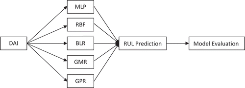
This section describes the different models used in developing the proposed approach to prognosis of slow rotating bearings. The entire condition-monitoring process is implemented in a unified framework (Figure 1). Generally, the process involves four main steps: (1) obtaining the degradation assessment index; (2) using the obtained DAI as input into MLP, RBF, BLR, GMR, and GPR, respectively; (3) the various models are then used for the RUL prediction of slow rotating bearings; (4) the five obtained models are evaluated to find out which of them gave the best prediction.

FIGURE 1 Framework for DAI integrated approach to bearing prognostics Key: DAI-degradation assessment index; MLP-multilayer perceptron; RBF-radial basis function; BLR-Bayesian linear regression; GMR-Gaussian mixture regression; GPR-Gaussian process regression; RUL-remaining useful life.

A Degradation Assessment Index

Providing a quantifying degradation indication for the assessment of machine performance is vital for prognosis. The degradation assessment index is obtained by the combination of the polynomial kernel principal component analysis (PKPCA), the Gaussian mixture model (GMM), and weighted moving average (EWMA). The PKPCA is a widely used technique for dimensionality reduction and feature extraction in machine learning (Schölkopf, Smola, and Muller 1998; 1999; Lee 2004). Subsequent to feature extraction by PKPCA from the high-dimensional statistics, the nonlinear (multimodal) features in low-dimensional data space can still be preserved. The polynomial kernel principal component henceforth, PKPC, which were extracted, are then used as inputs in the GMM, which is an outstanding technique of complex data description with benefits of high-performance computation and robustness. The GMM describes complex data distribution that often occurs in acoustic emission data by outputting the negative log likelihoods (NLL) utilizing numerous Gaussian components. The reliability and sensitivity of the NLL to the bearings’ slight degradation was improved by employing the exponentially weighted moving average (EWMA) statistic as an improved quantification index for prognostics of slow rotating bearings. The proposed EWMA is a kind of infinite impulse response filter applying exponentially decreasing weighting factors. Each older datum points weighting never reaches zero, decreasing exponentially. The resulting quantification index is named degradation assessment index (DAI). Therefore, in this study the DAI developed is used as a bearing degradation index in prognostics of slow rotating bearings.

Multilayer Perceptron Regression

The DAI is used as input into an MLP for the prognostics of slow rotating bearings in order to determine their RUL. MLP is one of the generally utilized architecture for empirical usage of neural networks. It more often than not comprises basically two layers of adaptive weights. There is a complete linkage connecting the inputs to the hidden units, as well as another connecting the hidden units to the output units (Nabney 2002).

The MLP is a mathematical function that has been parameterized by a set of numerical weights , ,…, , which we shall represent jointly by a vector of weight . The Bayesian technique entails inference of the posterior distribution of weights, , given data . It considers a functional probability distribution over the weighting space. The outputting prediction resulting from the input vector is then obtained by implementing a weighted sum of the predictions over all possible weight vectors, where the weighting coefficient for a particular weight vector is dependent on the posterior weight distribution. The predicted value is given as (Skabar 2007)

(1)

where is the MLP output, and is the predicted value.

The probability density function, , can be approximated using the fact that , where and are known, respectively, as the likelihood and the prior.

The prior weight distribution, , is the weight distribution before the observation of any data reflecting the prior knowledge of the MLP complexity. To obtain a smooth function for the reduction of the risk of overfitting, is assumed to be Gaussian with zero mean and inverse square variance , which gives:

(2)

where is the number of weights in the MLP. Because controls the value of other parameters (i.e., the weights) it is referred to as a hyperparameter.

Because the prior depends on , the modification of Equation (1) with the inclusion of the posterior distribution over parameters of the hyperparameters gives the predicted value as

(3)

where

(4)

Radial Basis Function Regression

Similarly, the DAI is used as input into radial basis function (RBF) regression for the prognostics of slow rotating bearing in order to determine its RUL. The RBF is used for nonlinear modeling. The RBF has many advantages, one of which is that it has a two-phase training process that is significantly quicker than MLP. In the first phase, the parameters of the bases functions are set to model the unconditional data density. In the second stage of training, the weights in the output layer are determined. Second, it is possible to assign an interpretation to the hidden units and also to determine the intrinsic degrees of freedom of the network (Nabney 2002). The RBF network mapping could be written in the following form, as shown in Equation (5).

(5)

where are the basis functions, and are the output layer weights.

The bias weights can be absorbed into the summation by including an extra basis function whose activation is constant value 1. This leads to Equation (6).

(6)

Two Bayesian approaches have been found to be effective, in practice, to neural networks (NN): Gaussian approximation to the posterior weight distribution in the weight space (known as the Laplace approximation) often coupled with use of the evidence procedure for optimal hyperparameter estimation; second, the Monte Carlo techniques, particularly the hybrid Monte Carlo (Nabney 2002).

Bayesian Linear Regression

The parametric approach focuses on the use of probability distributions having specific functional forms governed by a small number of adaptive parameters, such as the mean and variance, whose values are to be determined from the dataset. The probability distributions include beta (binomial) and Dirichlet (multinomial) distributions for discrete random variables and the Gaussian distribution and Gaussian mixture distribution for continuous variables. In this study the data is continuous, hence, the Gaussian distribution and Gaussian mixture distributions are considered (Bishop 2006). The Gaussian, also known as the normal distribution, is a widely used model for the distribution of continuous variables (Bishop 2006). For the case of a single real-valued variable, , the Gaussian distribution is given as

(7)

where , is known as the mean, and , is known as the variance.

The reciprocal variance is referred to as precision and is defined by

(8)

In this study, the acoustic emission signal is extracted at different operational conditions (speeds and dynamic loading conditions). A regression function, which measures the bearing vibration as a function of the different operating conditions, is fitted. The regression function is approximated based on the parameter prior and the data-driven likelihood. The prior indicates the characteristic nature of the functions of interpolation. As such, the prior allows for more vigorous interpolation functions, particularly if only noisy and limited data are obtainable.

An observation is given as the summation of the specific loading condition function as computed for the equivalent operational condition vector and the noise term .

(9)

The function of interpolation could be taken to an approximate linear dependency on x; if the operating conditional vector is adequately expressive, it might be necessary to make the assumption. The linearly dependent function is given by the parameter vector :

(10)

For the LSE solutions for the reference loading condition, a multivariate Gaussian distribution is approximated. This distribution is consequently utilized as the prior distribution p(w). Let the prior mean be taken as vector , and let the covariance matrix be taken as . Hence, the prior is given as

(11)

Based on Bayes’ theorem, the prior and the data determined likelihood are utilized in obtaining a posterior distribution for the values of parameters

(12)

where the posterior is normalized by the marginal likelihood . Prior probability is the probability available before the observation. However, posterior probability is the probability obtained after the observation. The likelihood function shows the possibility of the dataset observed for the settings of the vector of parameters. The posterior distribution could also be demonstrated to be a Gaussian distribution (Bishop 2006):

(13)

where the posterior mean and covariance for loading condition j is given by

(14)

(15)

The likelihood of the observation of a DAI value at an operational condition while traversing bearing time interval may be obtained from the recomputed likelihood function and is a type of a Gaussian (Bishop 2006):

(16)

The variance of the predictive distribution is indicative of the uncertainty in the prediction at an operational condition defined as

(17)

Gaussian Mixture Regression

In spite of the vital analytical properties of the standard single Gaussian distribution, it has some considerable limits in real-data modeling. If a dataset forms more than one dominant clump, the basic Gaussian distribution is incapable of capturing the structure, whereas the linear superposition of two or more Gaussians can give an improved description of the dataset. Such linear characterization, formed by taking a linear combination of more basic distributions such as Gaussians, can be formulated as probabilistic models known as mixture distribution (Bishop 2006).

In this study, a Gaussian mixture regression (GMR) is used to predict slow rotating bearing RUL from the DAI. Assume to represent the vector of the explanatory variables (e.g., operation conditions such as speed, time, load, etc.). The explanatory variables are those variables that may have impact on the signal characteristics, but that are generally independent of the bearing condition. The vector of the response or dependent variables (e.g., the DAI developed from extracted bearing features obtained from acoustic emission signal) is ; is the input training data , and is the output data . For the given and , the joint probability density is given as (Wang, Qian, and Guo 2013)

(18)

where

The probability density function (pdf) of the multivariate GMM is denoted by . Equation (18) shows that the relationship between the explanatory variables and the response variable can be can be described by several GMM models. The parameters of Equation (18) include the number of the mixture components, , the priors , the mean value , and the variance of each Gaussian component , which are represented as with and the constraint

As noted, each Gaussian component can be partitioned and the joint density can be rewritten as

(19)

Then marginal probability density of is

(20)

The conditional pdf of can deduced by combining Equations (19) and (20),

(21)

with the mixing weight

(22)

From Equation (22), the regression function for the prediction given a new input is

(23)

and the conditional variance function is

(24)

where

(25)

and

(26)

In Equation (23), is the GMR model of index , simply abbreviated as GMR(K) or . Although the regression function from the joint mixture Gaussian density is of the form of a kernel estimator commonly used in nonparametric models, the weight function is not determined by local structure of the data but by the components of a global GMM. Thus, the GMR is a global parametric model with nonparametric flexibility (Wang et al. 2013).

A major task in fitting the GMR is the estimation of the parameters, , of GMM for the joint density This can be achieved by maximizing the log likelihood function denoted as

(27)

For the given training data, the parameters (comprising the means, covariances, and missing coefficients) of a GMM is learnt by maximizing Equation (27) using the expectation maximization (EM) algorithm in the iterative means. There are some advantages to using the EM algorithm. The EM algorithm is simple to implement and understand, avoids the calculation and storage of derivatives, is usually faster to converge than general purpose algorithms, and can be extended to deal with datasets in which some points have missing values (Nabney 2002).

The EM algorithm includes two steps:

1. E step (expectation step):

   Calculate the posterior probability according to

   (28)

2. M step (maximum step):

   (29)
   (30)
   (31)

It is convenient to recast the maximizing problem in the equivalent form of minimizing the negative log likelihood of the dataset (Nabney 2002):

(32)

The two steps are iterated until the model converges to a local minimum (Calinon 2009). The entire dataset is divided into training and test sets. The training set is used in estimating the parameters of the GMM whereas the test set is kept for prediction of bearing damage and RUL. The results obtained may be highly sensitive to the number of mixing components used. The more components a mixture model has, the more expressive and flexible it becomes. A sufficiently expressive model may be optimized in order to accurately represent the reference signal. However, models that are too expressive might overfit the training data. This could result in poor generalization and subsequently impair the ability of the model to discern between normal signal components and fault-related outliers (Bishop 2006). Different numbers of mixing components (K) are fitted and the best is selected. There are several model selection criteria, such as the root mean square error (RMSE), the leave-one-out cross-validation technique (CV), the percentage prediction error (PE), the Bayesian information criterion (BIC), Bayesian model selection, and the Akaike information criterion (AIC), among others. In this study, the leave-one-out CV, was used to select the best number of mixing components. Given the test set, the GMR models can be obtained using the parameters of the GMM, which has an output of a smoothed general description of the GMM encoded data and linked constraints given by matrices of the covariance (Calinon 2009). This general smoothed description of the data is the prediction of the failure of the bearing.

Gaussian Process Regression

The use of Gaussian process regression (GPR) for prognosis (prediction of the RUL) of slow rotating bearings based on the DAI is possible. Gaussian processes (GP) are a recent development in nonlinear nonparametric modeling. In GP, the parametric model is dispensed and, instead, a prior probability distribution is defined over functions directly (Bishop 2006). A nonlinear functional mapping from an inputting space to a target space is achieved by the use of GP modeling. The GP is defined as an infinite collection of arbitrary variables of which any of the fixed subsets has joint Gaussian distributions. The Gaussian method is favorable for smoothing functions and those that properly explain the training data. The smoothing attribute of the function leads to its plausible generalizations (Heyns, de Villiers, and Heyns 2012).

To motivate the GP viewpoint, let the vector represent the DAI in the input space. The training set of inputting vectors corresponds to the targeted vector . For prognostics as in this study, is the time period and is a novel degradation assessment index for monitoring the health state of slow rotating bearings. A Gaussian process can be fully described by its mean and covariance (or kernel) function (Rasmussen and Williams 2006). These functions are specified separately and consist of a specification of a functional form as well as a set of parameters called hyperparameters.

The mean function describes the value of the function expected at any point of the inputting space, before the consideration of any trained data. The mean function can be defined as:

(33)

In supervised learning, the idea of likeness linking the various data points is vital. It is an essential similarity assumption that the points of inputs , which are in proximity to the target values , are expected to be similar. Hence, training points that are close to a test point’s prediction should be insightful. In the Gaussian process viewpoint, the covariance function depicts the nearness or similarity (Rasmussen and William 2006). The covariance function between two functional values evaluated at fixed points and is given as

(34)

The covariance function enables the inference value of a function given the knowledge of the other. Thus, the covariance function can be interpreted as the measure of the distance between the input points and . The Gaussian process can then be written as:

(35)

The basic GPR consists of a simple zero mean and squared exponential covariance functions. The zero mean function is given as

(36)

for every value of . One of the generally used kernel functions is the squared exponential (SE). It assumes that the function values in close proximity in the feature space are probably going to be similar, with close-to-unity covariance for variables that have feature inputs that are close. The squared exponential covariance function with automatic relevance detection is given as (Rasmussen and Williams 2006)

(37)

where matrix is diagonal with positive ARD parameters, and is length D vector corresponding to the input space dimension. The characteristic length-scale parameters, also known as the ARD parameters, determine the rate of variation of the function in the direction of the corresponding inputting space. A function tends to vary faster for any variation of its component feature for its shorter length-scale parameter for a specific feature component. A short length scale thus corresponds to high relevance; is the signal variance linked to the general function variance.

The free parameters (i.e., hyperparameters) in the covariance function can be compressed into a matrix denoted by . The values of these hyperparameters are all unknown and inference is made from the data being the trained. It can be shown by utilization of the Bayes’ rule that the maximum a posteriori hyperparameter values can be obtained by maximizing the marginal likelihood , which is the same as minimizing the negative log marginal likelihood (Rasmussen and Williams 2006):

(38)

where is the covariance matrix between all pairs of training inputs and is computed with Equations (5) or (6). It is important to note however, that the application in this study used an matrix of time points.

Given a set of training points, one can derive the posterior distribution over functions by imposing a restriction on prior joint distribution. Once a posterior distribution is derived, it can be used to estimate predictive values for the test data points (Saxena et al. 2009). Denoting as the training inputs and as the test inputs, prediction of at the new locations may be inferred by conditioning the joint distribution on the observed target values. For the basic GPR with zero mean, the following equations describe the predictive distribution (Rasmussen and Williams 2006).

Prior:

(39)

Posterior:

(40)

where

(41)

(42)

The maximum a posteriori (MAP) estimates can then be used as slow rotating bearing RUL metrics.

Model Evaluation

The models would be evaluated using MAPE and RMSE. The MAPE and RMSE between the predicted and the original DAI were calculated using Equations (43) and (44), respectively.

(43)

(44)

where is the actual value of the degradation assessment index for the ith observation, which is, in this case, the time point; is the predicted value of degradation assessment index; is the number of observations.

The leave-one-out CV technique was used in selecting the test set for validating the predictions from each model. Two approaches were considered. The first is based on dependent sample. In this approach the bearing dataset was divided into equal samples of training and test sets. The training set is the “seen” because it was used in training the parameters of the model, whereas the test set is the “unseen” because it was never fed into the model during training. However, it is been argued that when the training and test samples are dependent, the two errors may be positively correlated, resulting in a breakdown of the cross-validation selection approach, and can equally lead to model overfitting (Opsomer et al. 2001; Arlot 2010). Therefore, the second approach is based on independent samples, whereby two different sets of bearings are trained together and, hence, used as the training set while a third bearing dataset is used as the test set.

EXPERIMENTAL SETUP

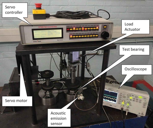
An experimental setup was used in this research to collect acoustic emission signals from a slow rotating bearing. The test setup was designed so that it would be able to test slow rotating bearings. The experimental test setup is shown in Figure 2 and was used in this study to collect the acoustic emission signals generated by slow rotating bearings. A controller controlled the rotational speed of the bearing. The system was driven by an AC servo motor with the speed set at 70 rpm, 80 rpm, and 100 rpm for bearings 1, 2, and 3, respectively. An acoustic emission sensor was mounted on the housing of the test Timken bearing.

FIGURE 2 Setup.

The life of the slow rotating bearings was tested until failure, which occurred on the outer race for all the bearings considered here. Ground metal debris was introduced gradually into Bearing 1 at the openings between the outer race, rollers, and inner race to accelerate the initiation of damage. Bearings 2 and 3 were simply not lubricated from the start to the end of the measurement process in order to speed up the bearing degradation. The slow rotating bearing was loaded at various dynamic loads by using an electrodynamic shaker. Bearing 1 was sinusoidally loaded over a range from 1.6 kN to −1.0 kN. Bearing 2 was loaded between 1.8 kN and −1.4 kN, whereas Bearing 3 was loaded between 2.0 kN and −1.7 kN. The excitation frequency was approximately 2 Hz.

The major components of the slow rotating bearing test setup are the Zonic Xcite 1100-4-FT System hydraulic shaker (load actuator), the load cell, the Timken tapered roller test bearings with bearing number HR 30307 J, the AC servo motor with model number 80MT-M04025, the speed controller and a National Instruments data acquisition card with a shielded BNC Connector Block.

The Soundwel acoustic emission sensor with model number SR 150 M was used for collecting the data in an analogue form. This broadband piezoelectric AE transducer was connected to a 40-dB gain preamplifier. The AE transducer was mounted on the outside surface of the outer race and on the bearing housing.

The frequency of interest was 100 kHz. Hence, the AE signal was recorded at a sampling frequency of 200 kHz over a sampling period of 1 s, using the NI PCI 6110 data acquisition card with the model occupying one of the ISA slots in a host computer. Data records were taken every 20 minutes until all three bearings failed, using the National Instruments Lab View software. The function for capturing the time domain and the preselected sampling time and interval was used. The recorded data was subsequently processed by means of dedicated MATLAB programs.

RESULTS AND DISCUSSION

Prediction Based on Dependent Samples

The predictions in this section are based on dependent observations whereby the training and the test sets are obtained using a leave-one-out CV technique that involves the division of the bearing dataset into equal samples of training and test sets.

The health state of a bearing is divided into three during its whole life: healthy or normal state, slightly degradation state, and failure state. There is no need for RUL when a bearing is in its healthy state. When the computed features are above their incipient damage threshold values, then it is considered that slight degradation has set in. The prediction model is then used in the prediction of the future value of the degradation assessment index.

In this investigation, healthy bearings are run until they are failed. A degradation assessment index is developed to assess the degradation of the slow rotating bearing. The DAI is then used in the several regression models: MLP, RBF, BLR, GMR, and the GPR models for prediction of bearing damage, RUL, and failure at a future instant of time.

Second, the MAPE and RMSE were used in model evaluation to select the best performing model. Third, the best performing model from the resulting novel methodologies is recommended and used for the prediction of slow rotating bearing remaining useful life.

RUL Using Multilayer Perceptron (MLP) Regression

Multilayer perceptron is one of the most frequently used feedforward artificial neural networks that make use of a supervised learning algorithm. Essentially, it has three layers, which include the input layer, pattern (hidden) layer, and output layer (Şengüler et al. 2010).

Dimensionality of the feature vectors was reduced to two PKPCs from five bearing extracted features using polynomial kernel principal components analysis (PKPCA), which subsequently fed into the GMM to obtain the degradation assessment index (DAI). The MLP neural network (NN) was trained with the DAI, which had been obtained from the bearing data at dynamic loadings conditions. The MAPE and RMSE between the predicted and the actual DAI are shown in Figures 3, 4, and 5 for Bearings 1, 2, and 3, respectively. The MLP NN approach was used to monitor the trend of the incipient bearing damage, and RULs of Bearings 1, 2, and 3 are shown in Figures 6(a), 7(a), and 8(a), respectively.

FIGURE 3 RMSE and MAPE for MLP, RBF, BLR, GMR, and GPR models for Bearing 1, based on the dependent samples.

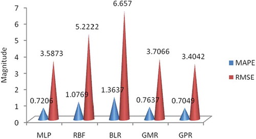
FIGURE 4 RMSE and MAPE for MLP, RBF, BLR, GMR, and GPR models for Bearing 2, based on the dependent samples.

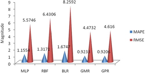
FIGURE 5 RMSE and MAPE for MLP, RBF, BLR, GMR, and GPR models for Bearing 3, based on the dependent samples.

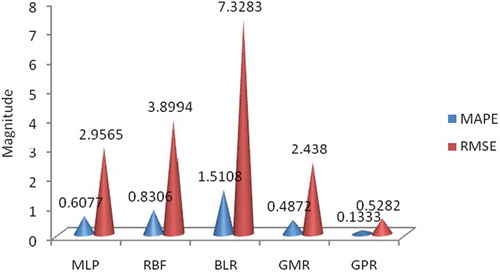
FIGURE 6 Prediction for the whole bearing life for Bearing 1 using different methodologies based on dependent samples.

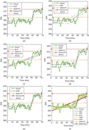
FIGURE 7 Prediction for the whole bearing life for Bearing 2 using different methodologies based on dependent samples.

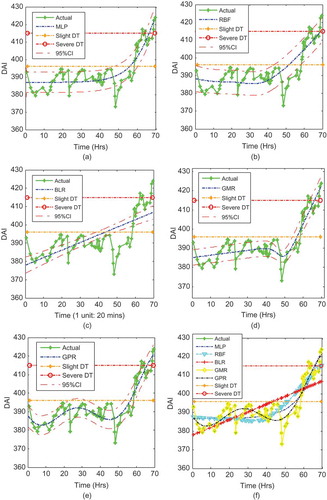
FIGURE 8 Prediction for the whole bearing life for Bearing 3 using different methodologies based on dependent samples.

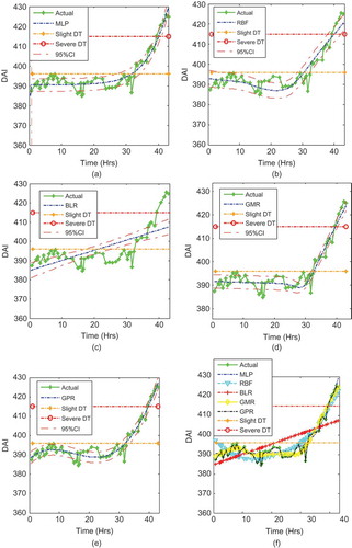
FIGURE 9 RMSE and MAPE for MLP, RBF, BLR, GMR, and GPR models for Bearing 1, based on the independent samples.

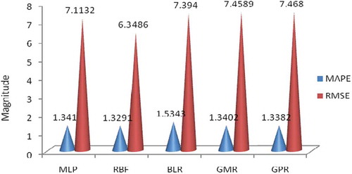
FIGURE 10 RMSE and MAPE for MLP, RBF, BLR, GMR, and GPR models for Bearing 2, based on the independent samples.

RUL Using Radial Basis Function (RBF) Regression

The RBF uses local hypersphere surfaces (nonlinear mapping) to separate the classes in the input space as a response to cluster, rather than the global hyperplanes (lines) used in MLP networks (Al-Raheem and Abdul-Karem 2010).

The degradation assessment index (DAI) was used as input into the RBF. The RBF was then trained with the DAI, which had been obtained from the bearing data at dynamic loadings conditions. The MAPE and RMSE were again computed between the predicted and the actual DAI and shown in Figures 3, 4, and 5 for Bearings 1, 2, and 3, respectively. The RBF predictions of the incipient bearing damage and RUL of Bearings 1, 2, and 3 were subsequently plotted as shown in Figures 6(b), 7(b), and 8(b), respectively.

RUL Using Bayesian Linear Regression (BLR)

Similarly, the degradation assessment index (DAI) was used as input into the BLR. The BLR was then trained with the DAI, which had been obtained from the bearing data at dynamic loadings conditions. The MAPE and RMSE were again computed between the predicted and the actual DAI and are shown in Figures 3, 4, and 5 for Bearings 1, 2, and 3, respectively. The BLR predictions of the incipient bearing damage and RUL of Bearings 1, 2, and 3 were subsequently plotted as shown in Figures 6(c), 7(c), and 8(c), respectively.

RUL Using Gaussian Mixture Regression (GMR)

Furthermore, the degradation assessment index (DAI) was used as input into the GMR. The GMR was then trained with the DAI, which had been obtained from the bearing data at dynamic loadings conditions. The MAPE and RMSE were again computed between the predicted and the actual DAI and are shown in Figures 3, 4, and 5, for Bearings 1, 2, and 3, respectively. The GMR predictions of the incipient bearing damage and RUL of Bearings 1, 2, and 3 were subsequently plotted as shown in Figures 6(d), 7(d), and 8(d), respectively.

RUL Using Gaussian Process Regression (GPR)

The degradation assessment index (DAI) was used as input into the GPR. The GPR was then trained with the DAI, which had been obtained from the bearing data at dynamic loadings conditions. The MAPE and RMSE were again computed between the predicted and the actual DAI and are shown in Figures 3, 4, and 5 for Bearings 1, 2, and 3, respectively. The GPR predictions of the incipient bearing damage and RUL of Bearings 1, 2, and 3 were subsequently plotted as shown in Figures 6(e), 7(e), and 8(e), respectively.

Model Evaluation of the Dependent Samples

After the training process, the prediction was done with data points equal to the training data points. The predicted and actual RUL plots of all the models were plotted and are shown in Figures 6(f), 7(f), and 8(f), respectively.

The MAPE and RMSE between the output and real values are observed as plotted in Figures 3, 4, and 5 for Bearings 1, 2, and 3 for all the five models: MLP, RBF, BLR, GMR, and GPR. All the models attempted to predict damage and RUL to a great degree.

For Bearing 1, the MAPE prediction errors from the models were 0.7049, 0.7206, 0.7637, 1.0769, and 1.3637 for GPR, MLP, GMR, RBF, and BLR, respectively, from the least to the highest prediction errors. Similarly, the RMSE prediction errors from the models were 3.4042, 3.5873, 3.7066, 5.2222, and 6.6570 for GPR, MLP, GMR, RBF, and BLR, respectively, from the least to the highest prediction errors. The worst prediction was that of the BLR, which was a linear line across the nonlinear model. The GMR and MLP also modeled damage and RUL with little error. However, the best predictive model for Bearing 1 was the GPR.

Similarly, for Bearing 2, the MAPE prediction errors from the models were 0.9206, 0.9233, 1.3171, 1.1554, and 1.6747 for GPR, GMR, MLP, RBF, and BLR, respectively, from the least to the highest prediction errors. Similarly, the RMSE prediction errors from the models were 4.616, 4.4732, 5.5746, 6.4306, and 8.2592 for GPR, GMR, MLP, RBF, and BLR, respectively, from the least to the highest prediction errors. The worst prediction was that of the BLR, which was a linear line across the nonlinear model. The GMR and MLP also modeled damage and RUL with little error. However, the best predictive model for Bearing 2 was the GPR.

Finally, for Bearing 3, the MAPE prediction errors from the models were 0.1333, 0.4872, 0.6077, 0.8306, and 1.5108 for GPR, GMR, MLP, RBF, and BLR, respectively, from the least to the highest prediction errors. Similarly, the RMSE prediction errors from the models were 0.5282, 2.438, 2.9565, 3.8994, and 7.3283 for GPR, GMR, MLP, RBF, and BLR, respectively, from the least to the highest prediction errors. The worst prediction was that of the BLR, which was a linear line across the nonlinear model. The GMR and MLP also modeled damage and RUL with little error. However, the best predictive model for Bearing 3 was the GPR.

It could be seen that the GPR model consistently had the least error for all three bearings. It was concluded, therefore, that the GPR model predicts damage and RUL better than the other models.

Predictions Based on Independent Samples

The predictions in this section are based on independent observations whereby two different sets of bearings are trained together and, hence, used as the training set while a third bearing dataset is used as the test set.

RUL Using Multilayer Perceptron (MLP) Regression

The MLP neural network was trained with the DAI, which had been obtained from the bearing data at dynamic loadings conditions. The MAPE and RMSE between the predicted and the actual DAI are shown in Figures 9, 10, and 11 for Bearings 1, 2, and 3, respectively. The MLP NN approach was used to monitor the trend of the incipient bearing damage, and RULs of Bearings 1, 2, and 3 are shown in Figures 12(a), 13(a), and 14(a), respectively.

FIGURE 11 RMSE and MAPE for MLP, RBF, BLR, GMR, and GPR models for Bearing 3, based on the independent samples.

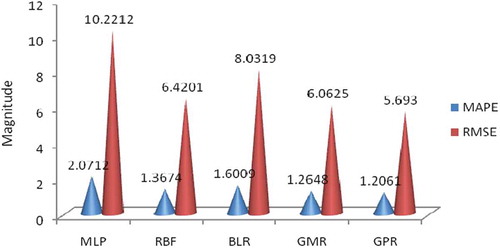
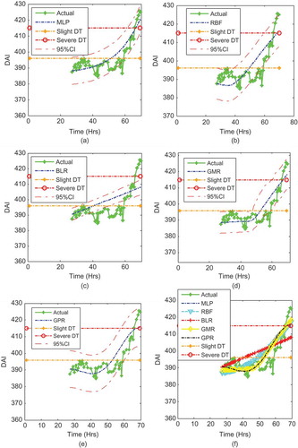
FIGURE 12 Prediction for the whole bearing life using Bearing 2 and 3 as training set and Bearing 1 as test set based on different methodologies and independent samples.

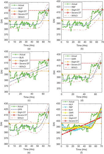
FIGURE 13 Prediction for the whole bearing life using Bearing 1 and 3 as training set and Bearing 2 as test set based on different methodologies and independent samples.

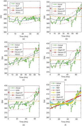
FIGURE 14 Prediction for the whole bearing life using Bearing 1 and 2 as training set and Bearing 3 as test set based on different methodologies and independent samples.

RUL Using Radial Basis Function (RBF) Regression

The degradation assessment index (DAI) was used as input into the RBF. The RBF was then trained with the DAI, which had been obtained from the bearing data at dynamic loadings conditions. The MAPE and RMSE were again computed between the predicted and the original DAI and are shown in Figures 9, 10, and 11 for Bearings 1, 2, and 3, respectively. The RBF predictions of the incipient bearing damage and RUL of Bearings 1, 2, and 3 were subsequently plotted as shown in Figures 12(b), 13(b), and 14(b), respectively.

RUL Using Bayesian Linear Regression (BLR)

Similarly, the degradation assessment index (DAI) was used as input into the BLR. The BLR was then trained with the DAI, which had been obtained from the bearing data at dynamic loadings conditions. The MAPE and RMSE were again computed between the predicted and the original DAI and are shown in Figures 9, 10, and 11 for Bearings 1, 2, and 3, respectively. The BLR predictions of the incipient bearing damage and RUL of Bearings 1, 2, and 3 were subsequently plotted as shown in Figures 12(c), 13(c), and 14(c), respectively.

RUL Using Gaussian Mixture Regression (GMR)

Furthermore, the degradation assessment index (DAI) was used as input into the GMR. The GMR was then trained with the DAI, which had been obtained from the bearing data at dynamic loadings conditions. The MAPE and RMSE were again computed between the predicted and the actual DAI and are shown in Figures 9, 10, and 11 for Bearings 1, 2, and 3, respectively. The GMR predictions of the incipient bearing damage and RUL of Bearings 1, 2, and 3 were subsequently plotted as shown in Figures 12(d), 13(d), and 14(d), respectively.

RUL Using Gaussian Process Regression (GPR)

The degradation assessment index (DAI) was used as input into the GPR. The GPR was then trained with the DAI, which had been obtained from the bearing data at dynamic loadings conditions. The MAPE and RMSE were again computed between the predicted and the actual bearing DAI and are shown in Figures 9, 10, and 11 for Bearings 1, 2, and 3, respectively. The GPR predictions of the incipient bearing damage and RUL of Bearings 1, 2, and 3 were subsequently plotted as shown in Figures 12(e), 13(e), and 14(e), respectively.

Model Evaluation Based on Independent Samples

After the training process, the prediction was done with data points equal to the training data points. The predicted and actual RUL plots of all the models were plotted and are shown in Figures 12(f), 13(f), and 14(f), respectively.

The MAPE and RMSE between the output and real values are observed as plotted in Figures 9, 10, and 12 for Bearings 1, 2, and 3 for all five models: MLP, RBF, BLR, GMR, and GPR. All the models attempted to predict damage and RUL to a great degree.

For Bearing 1, using the independent approach, the MAPE prediction errors from the models were 1.3291, 1.3382, 1.3402, 1.341, and 1.5343 for RBF, GPR, GMR, MLP, and BLR, respectively, for Bearing 1 from the least to the highest prediction errors. However, the RMSE prediction errors from the models were 6.3486, 7.1132, 7.394, 7.4589, and 7.468 for RBF, MLP, BLR, GMR, and GPR, respectively, from the least to the highest prediction errors. The worst prediction was that of the GPR model. The best predictive model for Bearing 1 was the RBF.

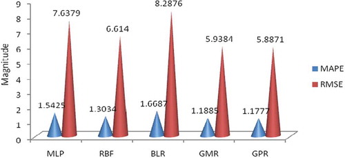
Similarly, for Bearing 2, the MAPE prediction errors from the models was 1.1777, 1.1885, 1.3034, 1.5425, and 1.5425 for GPR, GMR, RBF, MLP, and BLR, respectively, from the least to the highest prediction errors. Similarly, the RMSE prediction errors from the models were 5.8871, 5.9384, 6.614, 7.6379, and 8.2876 for GPR, GMR, RBF, MLP, and BLR, respectively, from the least to the highest prediction errors. The worst prediction was that of the BLR, which was a linear line across the nonlinear model. The GMR and RBF also modeled damage and RUL with little error. However, the best predictive model for Bearing 2 was the GPR.

Finally, for Bearing 3, the MAPE prediction errors from the models were 1.2061, 1.2648, 1.3674, 1.6009, and 2.0712 for GPR, GMR, RBF, MLP, and BLR, respectively, from the least to the highest prediction errors. Similarly, the RMSE prediction errors from the models were 5.693, 6.0625, 6.4201, 8.0319, and 10.2212 for GPR, GMR, RBF, MLP, and BLR, respectively, from the least to the highest prediction errors. The worst prediction was that of the BLR, which was a linear line across the nonlinear model. The GMR and RBF also modeled damage and RUL with little error. However, the best predictive model for Bearing 3 was the GPR.

Overall, the GPR model had the least error for all three bearings. It was therefore concluded that the GPR model predicts damage and RUL better than the other models.

Comparison of Model Performance Based on Dependent and Independent Samples

The ranks of each prediction model according to whether the training and tests samples are dependent or independent are presented in Tables 1, 2, and 3 for Bearings 1, 2, and 3, respectively. Although some of the models are sensitive to the type of sample, others are not. For example, the GPR and BLR models ranked mainly first and last, respectively, in both the dependent and independent samples, whereas RBF and MLP ranked differently. However, the errors obtained from the cross-validation based on independent samples (see Figures 9 to 11) were relatively larger than those from the dependent samples (see Figures 3 to 5), which could be an indication that the latter slightly overfitted the models.

TABLE 1 Ranking of Models Based on Dependent and Independent Samples for Bearing 1

	Dependent Samples		Independent Samples
Models	MAPE	RMSE	MAPE	RMSE
GPR	1	1	2	5
GMR	3	3	3	4
RBF	4	4	1	1
MLP	3	2	4	2
BLR	5	5	5	3

TABLE 2 Ranking of Models Based on Dependent and Independent Samples for Bearing 2

	Dependent Samples		Independent Samples
Models	MAPE	RMSE	MAPE	RMSE
GPR	1	2	1	1
GMR	2	1	2	2
RBF	4	4	3	3
MLP	3	3	4	4
BLR	5	5	5	5

TABLE 3 Ranking of Models Based on Dependent and Independent Samples for Bearing 3

	Dependent Samples		Independent Samples
Models	MAPE	RMSE	MAPE	RMSE
GPR	1	1	1	1
GMR	2	2	2	2
RBF	4	4	3	3
MLP	3	3	5	5
BLR	5	5	4	4

CONCLUSION

This article proposes a novel approach to damage detection and prediction of remaining useful life of slow rotating bearings. During this investigation, three healthy slow rotating bearings were run to the point of failure. A degradation assessment index, DAI, which was obtained by the integration of polynomial kernel principal component analysis (PKPCA), Gaussian mixture model (GMM), and exponentially weighted moving average (EWMA) was used in slow rotating bearing prognostics. The slight and severe degradation thresholds are obtained through the use of the kernel density estimation (KDE) technique on the healthy and slightly degraded bearing data, respectively. The DAI is used in the prediction of bearing damage and RUL using the MLP, RBF, BLR, GMR, and GPR models, respectively. Predictions were obtained using test and training sets from both dependent and independent samples. The models were able to predict damage and RUL of the slow rotating bearing. Overall, the GPR had the least mean absolute percentage and root mean square errors in this investigation for the slow rotating bearings and is robust to dependent and independent samples under varying operating conditions. Hence, the GPR is chosen as the most efficient model for prediction of RUL of slow rotating bearings. This proposed approach is useful and its application can be extended to the condition monitoring of other mechanical and allied systems.

REFERENCES

- Al-Raheem, K. F., and W. Abdul-Karem. 2010. Rolling bearing fault diagnostics using artificial neural networks based on Laplace wavelet analysis. International Journal of Engineering, Science and Technology 2(6):278–290.
- An, D., J.-H. Choi, and N. H. Kim. 2012. A comparison study of methods for parameter estimation in the physics-based prognostics. Paper presented at the Annual Conference of Prognostics and Health Management Society, Minneapolis, Minnesota, USA, September 23–27, 2012.
- An, D., N. H. Kim, and J.-H. Choi. 2013. Options for prognostics methods: A review of data-driven and physics-based prognostics. Paper presented at the Annual Conference of the Prognostics and Health Management Society, New Orleans, October, 14–17, 2013.
- Arlot, S. (2010) A survey of cross-validation procedures for model selection. Statistics Surveys 4:40–79.
- Bishop, C. M. 2006. Pattern recognition and machine learning. Cambridge, UK: Springer.
- Bolander, N., H. Qiu, N. Eklund, E. Hindle, and T. Rosenfeld. 2009. Physics-based remaining useful life prediction for aircraft engine bearing prognosis. Paper presented at the Annual Conference of the Prognostics and Health Management Society, San Diego, CA, September 27 – October 1, 2009.
- Calinon S. 2009. Robot programming by demonstration: A probabilistic approach. EPFL/CRC Press, 2009.
- Camcia, F., K. Medjaher, N. Zerhounib, and P. Nectoux. 2012. Feature evaluation for effective bearing prognostics. Quality and Reliability Engineering International 29(4):1–15.
- Chatzis, S. P., D. Korkinof, and Y. Demiris. 2012. A nonparametric Bayesian approach toward robot learning by demonstration. Robotics and Autonomous Systems 60(6):789–802.
- Chen, T., and J. Ren. 2009. Bagging for Gaussian process regression. Neurocomputing 72(7–9):1605–1610.
- Gebraeel N., M. Lawley, R. Liu, and V. Parmeshwaran. 2004. Residual life predictions from vibration-based degradation signals: A neural network approach. IEEE Transactions on Industrial Electronics 51:694–700.
- Goebel, K., B. Saha, and A. Saxena. 2008. A comparison of three data - driven techniques for prognostics. Paper presented at the Proceedings of the 62nd Meeting of the Society For Machinery Failure Prevention Technology (MFPT), Virginia Beach, VA, May 6–8.
- Heyns, T., J. P. de Villiers, and P. S. Heyns. 2012. Consistent haul road condition monitoring by means of vehicle response normalisation with Gaussian processes. Engineering Applications of Artificial Intelligence 25(8):1752–1760.
- Hippert, H. S., and J. W. Taylor. 2010. An evaluation of Bayesian techniques for controlling model complexity and selecting inputs in a neural network for short-term load forecasting. Neural Networks 23:386–395.
- Hong, S., and Z. Zhou. 2012a. Remaining useful life prognosis of bearing based on a Gaussian process regression. Paper presented at the 5th International Conference on BioMedical Engineering and Informatics (BMEI 2012), Chongqing, China, October 16–18, 2012.
- Hong, S., and Z. Zhou. 2012b. Application of Gaussian process regression for bearing degradation assessment. In Proceedings of the information science and service science and data mining (ISSDM) 2012, 6th international conference on new trends, 644–648. ISSDM/IEEE.
- Jardine, A. K., D. Lin, and D. Banjevic. 2006. A review on machinery diagnostics and prognostics implementing condition based maintenance. Mechanical Systems and Signal Processing 20(7):1483–1510.
- Lee, J.-M., C. Yoo, S. W. Choi, P. A. Vanrolleghem, and I.-B. Lee. 2004. Nonlinear process monitoring using kernel principal component analysis. Chemical Engineering Science, 59:223–234.
- Liu, D., J. Pang, J. Zhou, and Y. Pang. 2012. Data driven prognostics for Lithium-ion battery based on Gaussian process regression. Paper presented at the 2012 Prognostics and System Health Management Conference (PHM-2012), Beijing, China, May 23–25.
- Malhi, A., and R. X. Gao. 2004. PCA-based feature selection scheme for machine defect classification. IEEE Transactions on Instrumentation and Measurement 53(6):1517–1525.
- Marble, S., and B. Morton. 2005. Predicting the remaining life of propulsion system bearings. In Proceedings of IEEE Aerospace Conference. IEEE.
- Nabney, I. T. 2002. NETLAB algorithms for pattern recognition. Great Britain, UK: Springer.
- Opsomer, J., Y. Wang, and Y. Yang. 2001. Nonparametric regression with correlated errors. Statistical Science 16(2):134–153.
- Rasmussen, C. E., and C. K. I. Williams. 2006. Gaussian processes for machine learning. Cambridge MA: MIT Press.
- Saha, B., K. Goebel, and J. Christophersen. 2009. Comparison of prognostic algorithms for estimating remaining useful life of batteries. Transactions of the Institute of Measurement & Control 31(3–4):293–308.
- Saxena, A. 2010. Prognostics, the science of prediction. Paper presented at the Annual Conference of the Prognostics and Health Management Society, Portland, OR, October 10–14, 2010.
- Saxena, A., J. Celaya, B. Saha, S. Saha, and K. Goebel. 2009. On applying the prognostic performance metrics. Paper presented at the Annual Conference of the Prognostics and Health Management Society, San Diego, CA, September, 2009.
- Schölkopf, B., A. Smola, and K. R. Muller. 1998. Nonlinear component analysis as a kernel eigenvalue problem. Neural Computation 10:1299–1319.
- Schölkopf, B., A. Smola, and K. R. Muller. 1999. Kernel principal component analysis. In Advances in kernel methods - Support vector learning, 327–352. Cambridge, MSA: MIT Press.
- Şengüler, T., Karatoprak E. and Şeker S. 2010. A new MLP approach for the detection of the incipient bearing damage. Advances in Electrical and Computer Engineering 10(3):34–39.
- Si, X. S., W. Wang, C.-H. Hu, and D.-H. Zhou. 2011. Remaining useful life estimation- A review of the statistical data driven approaches. European Journal of Operational Research 213:1–14.
- Skabar, A. 2007. Mineral potential mapping using Bayesian learning for multilayer perceptrons. Mathematical Geology 39: 439–451.
- Wang, G., L. Qian, and Z. Guo. 2013. Continuous tool wear prediction based on Gaussian mixture regression model. International Journal of Advanced Manufacturing and Technology 66:1921–1929.
- Wang, M., and J. Wang. 2012. CHMM for tool condition monitoring and remaining useful life prediction. International Journal of Advanced Manufacturing and Technology 59:463–471.