An Approach to Intelligent Traction Control Using Regression Networks and Anomaly Detection

Abstract

This article discusses an intelligent driving system (IDS) that uses a Polynomial Regression Network (PRN) and a Gaussian Anomaly Detection System (GADS). The PRN models the relation between the motor input and vehicle movement, thus, inherently taking nonlinear and noisy environmental factors into consideration. The anomaly detection system detects probable system output or sensor failure using a Gaussian pattern-match algorithm for taking proper corrective action. The time of computation for training the PRN is shown to be as low as 0.3 seconds and thus, the system can be used for instantaneous training in any environment at high speeds. Such intelligent driving systems will be useful for electric race-car designs, electric consumer vehicles, and robotic vehicles for stability on adverse road or track conditions.

INTRODUCTION

Electric vehicles (EVs) and Hybrid Vehicles (HVs) are much of interest in the world recently, especially in the domains of formula racing cars. This article emphasizes the application of an intelligent traction control and driving system in an EV. Traction control is achieved via differentials that alter wheel speeds for stability during turns and bends. There are two types of differentials as discussed in the literature: electronic and mechanical. In an electric vehicle, electronic differential is preferred over mechanical differential because of its lower weight and good speed maneuverability, which drastically enhances the performance of an EV dynamically, as well as in terms of safety. Numerous novel designs can be made for an electric vehicle with electronic differential, because speed manipulation can be achieved electronically, which increases the performance and safety of the EV.

Traction control concepts using various techniques and algorithms are common in the literature. These include direct torque control (DTC), direct torque fuzzy control (DTFC), neural networks PID, PI control and recurrent neural networks control (RNN).

Hartani et al. (2008) in direct torque control of an electronic vehicle determined the amount of stator flux of permanent magnet synchronous motor (PMSM) required for generating a given amount of torque. Hartani et al. (2009) uses fuzzy logic controllers, which overcomes the drawbacks of their previous work such as reducing the torque ripples, etc.

Fu et al. (2012), used accelerometer at the center of mass of the vehicle to determine the yaw rate and vehicle side-slip angle. They implemented a closed loop system, which is quite stable, but has no self-learning algorithms.

Haddoun et al. controlled differential drive using recurrent neural networks (RNNs) to model an induction motor. The RNN models the relation between input current and output torque and thus, is a kind of direct-torque-controlled electronic differential. The RNN relates the current required by the motor to the torque developed by it, but the actual movement of the vehicle was not taken into consideration. Two-wheel drive control by Zhao, Zhang, and Guan (2011) uses the slip formula proposed by them, which is controlled by a fuzzy logic-based controller.

Works on neural networks PID controller for electronic differential (Zhai and Dong 2011) and PI control of electronic differential using slip (Vitolis and Galkin 2012) are also found in the literature. Although PI/PID controllers are widely used in industry, it works fine only in very controlled environments and fail to perform if external nonlinear and noise factors are present.

Again, although RNNs and ANNs have been used for traction control, direct torque control takes care of the nonlinear factors in the motor and not the environmental factors such as friction, wheel slip, etc. Thus, although the exact torque might be provided by the system, it is not guaranteed that the vehicle will move the exact expected value for the given amount of torque. This article attempts to rectify the problem by directly modeling the movement of the car with the motor pulse width modulation (PWM) input.

In this article, a new system of operation has been proposed. It uses a combination of a polynomial regression network (PRN) and a Gaussian error detection algorithm for a complete driver assistive system. PRNs are much faster to train and, thus, can be trained instantaneously at any environment at high speeds.

BASIC CONCEPTS

In any straight driven vehicle, the area of contact of all the tires with ground will be different due to uneven load distribution of the vehicle, uneven road conditions, and other environmental conditions such as friction. Due to this, even if all the tires of the vehicle move with the same speeds, the vehicle might not move the desired path because of wheel slip. Again, for a vehicle making a turn, differential speeds are required to be fed to the wheels. This is because of the basic fact that , where r is the distance between the center of the radius of curvature and the tire. This distance, r, is less for the inner tire and more for the outer tire when the vehicle is making a turn, and thus, differential speeds are required at the two wheels for proper and stable turning. Although the required speeds can be calculated by the theoretical formula, the theoretical speeds will not always hold for an uneven or noisy environment. Also, the vehicle will not always move the required amount for a particular PWM input. For rectifying such problems, ANNs, RNNs and PRNs are used that model the exact relation between vehicle movement and PWM input for a particular environment.

Electronic Differential

An electric vehicle with electronic differential is better compared to that with a mechanical differential, not only because the weight of the vehicle reduces, but also because the speeds of the two wheels can be better controlled with an intelligent algorithm. In the case of a mechanical differential, intelligent control cannot be achieved because it is impossible to implement ANNs, RNNs or PRNs to alter the speed of the wheel. Thus, the speed differences of the wheels will be fixed according to theoretical calculations. Such a differential system will have no self-learning scope and, thus, will not cater well in all types of environments and situations. But, in the case of an electronic differential, the speed of the wheels can be altered intelligently using PWM inputs. The PWM inputs can be determined by any advanced self-learning intelligent algorithm.

Advanced Learning Techniques

Various advanced machine learning techniques are available in the literature. Regression models, neural networks, support vector machines, and others can all be used to learn complex datasets. Machine learning is broadly divided into prediction and classification problems (Ng, No. 17, 2013a). Classification problems include prediction of probability of an event to occur. Prediction problems generally include prediction of a value by matching the pattern of the input training data. The problem presented in this article is an example of a prediction problem. The machine learning algorithm needs to figure out a pattern between the input PWM and the output movement of the car. From this pattern, the algorithm will predict the PWM input required for a certain required car output.

In the case of classification problems with a sigmoid activation function, neural networks with multiple layers have a far better accuracy than regression models (98% compared with 95% for handwritten digit classification). But ANNs are somewhat code and machine dependant as the training depends on the randomization of the initial weights (Smith and Mason 1996). Moreover, as was seen, ANNs had lesser accuracy in cases of prediction problems compared to polynomial regression models in this article. So, regression networks were chosen for use in this article. Regression models have a slightly faster training time due to the simplicity of code and the absence of backpropagation.

Optimization is the most important part of a learning model. It is the step where the objective cost function is minimized. Gradient descent, stochastic descent, and batch descent are the commonly used optimization techniques. Although stochastic and batch descent have faster training times, they are generally used for very large datasets only and generally have a lower accuracy. This is because, in the case of stochastic descent, the algorithm might not always converge to the optimal minimum, but might wander around it. Thus, gradient descent is a perfect choice for such an application (Ng, No. 17, 2013a).

This article uses polynomial regression as the learning technique along with gradient descent for optimization. The main points to be noted during such a process are

• Choice of polynomial features

• Choice of lambda

• Choice of training data

A number of polynomial features will determine the accuracy, overfitting, and underfitting of the algorithm on the dataset. Higher numbers of polynomial features will result in a more complete modeling of all the data points but might also result in overfitting, in which the data fits an unnecessary higher polynomial degree curve. Such overfitting of data results in a high error on the test set although the training set error is very low. To compensate for this, a regularization parameter lambda is chosen. The best value of lambda and the number of polynomial features should be chosen on the basis of the lowest difference in error between the test and training set (Ng, No. 10, 2013b)

The training data is ideally chosen such that all possible cases are modeled. But, such a training dataset is impossible in the case discussed in this article; because the training is instantaneous and in real time, it will be seen that even a certain fraction of the training data will also have a fairly good amount of accuracy.

Anomaly Detection as an Unsupervised Learning System

Anomaly detection refers to algorithms that detect an unusual set of values or an unusual behavior of a system. Such algorithms may be classified as an unsupervised, a semisupervised, or a supervised learning algorithm (Chandola, Banerjee, and Kumar 2007). For such an application, a supervised approach might not be feasible because there might be infinite error possibilities. Thus, the algorithm has to detect an unusual set of values compared with the assumed majority normal values seen. In such an unsupervised approach, Gaussian pattern match can be used to compute the pattern match of a dataset with the majority normal values. Thus, anomalies that are rare can be best detected by the Gaussian pattern-match algorithm. The classification of a dataset as an anomaly depends on how much the threshold of minimum pattern match percentage is fixed (Ng, No. 15, 2013c).

THE DIFFERENTIAL MODEL

Electronic differential models are commonly expressed in the form of mathematical expressions for the angular velocities of the right and left wheels.

At higher speeds, wheel abrasion, and air friction affect the angular velocities of the system. The PRN takes the aforementioned factors into account and predicts the actual angular velocities required. In the following differential model, for calculating the angular velocities for particular steering values, the wheel base () is assumed as 1.6 meters and track width () as 1.25 meters. The steering angle is restricted between −135 degrees to +135 degrees, and front wheel angle () is restricted to 32 degrees. The gear ratio for the steering wheel, based on the assumed system parameters is 4.21875:1.

From Figure 1, the expressions for the right and left wheel velocities are derived as

(1)

where

FIGURE 1 Basic electronic differential model.

	=	= Linear velocity of left rear wheel
	=	= Track width of the vehicle
	=	= Angular velocity of the vehicle
	=	= Horizontal distance between center of turn to the center of the track width

(2)

where = Linear velocity of right rear wheel

(3)

where

	=	= Wheel base of the vehicle
	=	= Front wheel angle

Now, the rear wheel velocities can be written as

(4)

where = Angular velocity of left rear wheel.

(5)

where = Angular velocity of right rear wheel.

The front wheel angular velocities will be the linear velocity of the vehicle.

(6)

(7)

where

f-l	=	= Angular velocity of the front left wheel
f-r	=	= Angular velocity of the front right wheel

Thus, the front wheel angular velocities and the linear velocities are known. So, for a particular velocity and steering angle, there exists an ideal set of rear wheel and front wheel angular velocity values.

INTELLIGENT CONTROL

This article proposes to use a self-learning polynomial regression network (SLPRN) and a Gaussian anomaly detection system (GADS) for intelligent traction control and accident prevention. SLPRN creates a modeling of the highly complex function of vehicle movement in terms of PWM input to motors. This is because the SLPRN cares only about the output and trains itself to achieve the desired output. Thus, the process automatically takes into consideration the nonlinearities of the motor and the inherent environmental factors such as friction, slip, etc.

In combination with SLPRN, it is proposed to use a Gaussian anomaly detection algorithm, which is used for the detection of an anomalous set of sensor values. Such an algorithm will safeguard the driver against false neural network corrections due to junk sensor readings and sensor failure.

Operation of PRN

The stability of a vehicle can be judged by the front and rear wheel velocities. As the rear wheels are driven and the front wheels follow, the velocities of front wheels gives an idea of actual vehicle movement. If the rear wheels move and the front wheels don’t, it may indicate the vehicle is skidding or slipping. Thus, the relation between the rear wheel and front wheel velocities will give an idea of vehicle stability. In the ideal situation model, it has been calculated and shown that for every particular rear wheel velocity and turning angle, there exists an ideal pair of front wheel angular velocities. Thus, it can be said for a particular PWM input to the driving motors at a particular steering angle, there exists a set of ideal front wheel values for which the vehicle will have the desired movement and be stable. But, due to various environmental factors, the angular velocity of the front wheel will never be equal to the predicted value for a particular PWM input to the motor. So, the objective function of the PRN is to model the relation between the front wheel velocities and the PWM input to the motor for a particular environment. Such a relation will relate the actual vehicle movement with the motor input, taking care of nonlinearities in the motor and the particular environmental factors inherently. The flow of the operation is shown in Figure 2.

FIGURE 2 Overall flow of operation.

The learning data required is automatically gathered pretraining. After training, the PRN, for the particular instant of environmental conditions, is made to predict the PWM value for the required ideal angular velocities of the front wheels. The predicted PWM input to the motors will be the desired input for obtaining the desired stable vehicle movement in that scenario. In this process, it is assumed that data gathering and training time required is fast enough that it doesn’t cause any observable delay.

As shown in Figure 3, training of the PRN is done using car velocity, steering angle, and the front wheel speeds as the input layer and the PWM values of rear left and right wheels as the output layer. As training starts, the system acquires the front wheel speeds for a sweep of input PWM values from zero to a few values above the present PWM input. The upper limit is fixed to a few values above the present value to avoid any unsafe velocity spikes. The PRN is then trained using a linear regression by using a suitable optimization technique such as gradient descent. The flow of training is as illustrated in Figure 4.

FIGURE 3 PRN structure.

FIGURE 4 Flow of PRN.

The output layer error is calculated as

(9)

where represent the predicted output and represent the training output data.

The expression for the output according to the implemented PRN can be written as

(10)

where

and

X represents the vector of input terms and their polynomial terms and the vector represents the coefficients of all the terms. The optimal coefficients model the output in terms of the input parameters. The cost function can be minimized using gradient descent where the gradient is calculated as

(11)

where

The gradient descent algorithm will iterate the value of theta according to the gradient of the cost function to arrive at the local optimum, i.e., the best fit to the training data.

(12)

The iterations are run until a maximum set value of 500 for this case, but the iterations stop if a local optimum has already been found before 500 iterations.

From the ideal vehicle calculations, the front wheel velocities for a particular steering angle and car velocity are known. The neural network is made to predict the required PWM values by feedforwarding input values with the required ideal front wheel speed values. This output inherently takes into consideration the innumerous environmental factors and, thus, is accurate.

Anomaly Detection

While running, the vehicle behavior error is constantly calculated as

(13)

where represents the real left- and right-wheel speed values, and represents the ideal/required left and right wheel speed values.

If the error is persistent for a time greater than a set threshold, an anomaly is detected. This suggests the pretraining of the neural network is not suitable for the present scenario. In such a case, the PRN is trained on the spot for minimizing the stability function. It is assumed that processor speed is high enough such that the training time is less than the motor speed update time for maintaining stability. For real emergency scenarios, this time can be of the order of milliseconds.

The sensor values are also fed into another independent anomaly detection system that detects anomaly in the sensor data. Anomaly in sensor data suggests probable sensor failure, and override code is triggered in such a case. The anomaly detection system is a commonly used Gaussian pattern-matching algorithm that declares output as an anomaly when the set of sensor readings doesn’t follow the normal pattern. The sensor readings are compared with mean and standard deviation of the previous sensor values and are used for computing pattern boundary.

(14)

(15)

For an input , the pattern match is computed using the formula

(16)

where, = the length of the input , i.e., the number of features present in the ith input vector.

The probability of an anomaly is computed if the pattern match is below a certain calibrated threshold, epsilon ().

Override Code

There are many methods of controlling the vehicle using the electronic differential system (EDS) as already discussed, but still, there is a finite probability that the sensor or the input parameters used for the EDS might be damaged due to extrinsic or the intrinsic factors. In such a case, the EDS takes in the wrong values and the control algorithm provides a solution that is totally different from the required solution. In simple language, the EDS fails in this case, and the EV becomes vulnerable to accidents, especially during the events such as turning. In this article, the problem is solved by detecting the anomalies in the sensor readings using the Gaussian pattern-matching method. When the anomaly is detected from this method, a new control algorithm (override code) will take control of the vehicle and accidents can be prevented.

Override Code Algorithm

Failure of any sensor associated with giving of angular values of wheels will output an anomalous/absurd value. This absurdness will be detected by the Gaussian pattern-matching method in the processor. The override code will take control of the EV depending upon the working sensor inputs (steering angle and linear velocity). Hence, the EV is safely controlled even if the EDS fails, as proposed in the following steps:

• The values from the input sensors are stored in a memory for each cycle when all the sensors are perfectly working for a certain period of time (Ts).

• The angular velocity sensor feedback loop is cut off once failure is detected and confirmed. The steering angle and linear velocity input is fed to the PRN and the previous best values of PWM signals are outputted.

• The previous best training fit is chosen on the basis of least stabilization time.

• The driver will be pinged of the failure so that he/she may take appropriate action.

SIMULATIONS AND TESTING

The algorithm was tested on a 2 GHz, Intel Core i5 system on a MATLAB environment. As the algorithm needs real-time testing for it to be proven, we synthesized model data and trained our neural network on it to prove the working principle.

PRN

The algorithm was tested with ideal data calculated with steering angle and velocity of four wheels as input; and PWM_l (left-wheel PWM) and PWM_r (right-wheel PWM) as output. During testing, the training data was generated using values for PWM input with the front wheel velocities for the particular environment. Now, the ideal front wheel velocity was inputted to the PRN and it outputted the particular PWM input required to achieve the required front wheel velocity. This proves that during training, the PRN will learn from that instantaneous environment, the relation between the PWM input and the actual vehicle movement.

As is seen from Figure 5, the training set error and the total error (i.e., the error of the entire training and test set) slowly converge. This suggests proper training of the data and that the fit is not an underfit or an overfit. It is noted that the difference between the total and the training set errors remains fairly constant after about 20 examples. As shown in Table 1, we used a mere 36 examples only for training our model, yet still achieving a robust accuracy. Our training data was arranged in increasing order of speed. Thus, the first 15 examples were up to a speed of about 20 kmph. Even with such a small training dataset, the algorithm predicts with an error of about 1 in an output range of 0–255. Thus, the algorithm can be trained on the spot at any speed by generating a rapid sweep of input from zero to the current speed value. There is no need to generate the entire possible sweep of speed input values, which could cause hazards of a sudden overshoot.

TABLE 1 No. of Training Data vs Error and Timec

No. of Training Data	Error (%)	Training Time (secs)
36	1	0.7

FIGURE 5 Test error and training error vs. training examples.

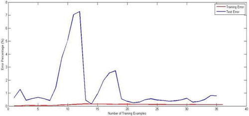
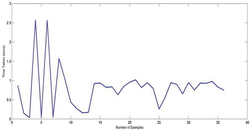
A fluctuation in time is also noted with varying numbers of training examples in Figure 6. This shows that the time required for reaching the local optimum varied with the number of examples being trained. This was because for a certain number of training examples, the data contained was in sufficient to model a particular equation based on the polynomial input in this case. However, the worst case time taken after 20 training examples was about 1 second, and the average time was about 0.5 to 0.7 seconds. Such a training time is pretty fast in the real scenario, and thus, the algorithm can be applied to a car at high speeds.

FIGURE 6 Training time vs. number of examples.

In the modeling of the PRN, there are a certain number of design parameters such as choice of polynomial features and choice of regularization parameter, lambda. The optimal values of the two are chosen such that the error and training time are the least.

Choice of Number of Polynomial Features

The increase in the number of polynomial features greatly affects and improves accuracy as the nonlinear relations are then accurately modeled.

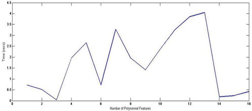
It is again noted from the table that the training time suddenly increases at first and then reduces drastically. This is because, at that certain number of polynomials, the local minimum was diffiuclt to find. In other words, the program exceeded the maximum iteration values to obtain the theta and there was no guarantee that the obtained weights were the best. As in the second case, a local minimum was possible, but it was reached after many iterations and thus, the time required was high. Thus, the polynomial terms involved in either case were not sufficient to exactly model the relation between the input and output layers. We see at six polynomial features the time required drastically reduces as the program is easily able to find the local minima and thus the best weight for modeling the input and output layers.

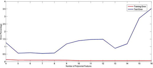
For proper evaluation of the model, the data was separated into the training and test set in the ratio of 3:1. The training and test set errors give an idea for choosing the best parameters. The plot in Figure 7 shows the training and test set error with the increase in the number of polynomial features. A small difference between the two errors indicates a perfect fit and thus, the number of features of from five to eight provides a suitable fit.

FIGURE 7 Training and test error vs. number of polynomial features.

Time required for training is also a factor for choosing the number of polynomial features. From the plot in Figure 8, it is seen that the training time and the error are the least at six polynomial features. Thus, at six polynomial features, the local optimum was found pretty easily and the relationship was perfectly modeled, as is depicted in Table 2.

TABLE 2 Error vs. No. of Polynomial Features

No. of Polynomial Features	Error %	Training Time (secs)
6	0.6	0.7

FIGURE 8 Training time vs. number of polynomial features.

Choice of Lambda

The regularization parameter, lambda is an essential parameter because it prevents overfitting. Overfitting will output predictions although the error on the training set will be low. Thus, the best value of lambda can be chosen on the basis of the plot between the test set and training set error (Figure 9). The lambda for which the least difference is present between the two errors is the best lambda. The algorithm was tested with lambda ranges varying from 0.1 to 100. The best lambda was found to be around 40.

FIGURE 9 Training and test set error with varying lambda.

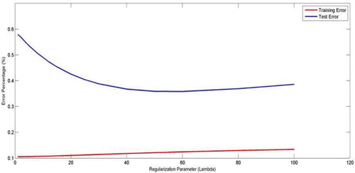
Another concerning factor for choosing lambda is the training time. A lambda value of 40 gave a pretty low training time of about 0.5 seconds and, thus, was perfect for the dataset.

Final Results

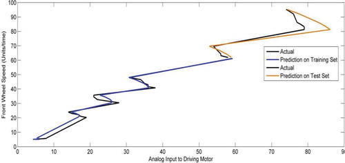
The graph of the actual vehicle movement in terms of the front-wheel speeds was plotted against the motor analogue input in Figure 10. The first two-thirds of the data was fed to the PRN for training. The PRN predicted the vehicle movement for the training set, as well as for the test set, successfully.

FIGURE 10 Actual front wheel movement vs. PRN prediction.

Anomaly Detection

The Gaussian pattern-detection algorithm was successful in predicting a randomly fed anomalous sensor value. The system was fed with normal sensor value data of the steering angle, and the four wheel speeds; 807 normal sensor readings were fed along with 5 anomalous values. The algorithm predicted the five values as an anomaly because it failed to match the majority pattern.

Whether a particular reading is a mismatch depends on the threshold factor chosen. This threshold factor defines the minimum match percentage for a reading to be called normal. Below the threshold, the reading is said to be an anomaly. Thus, a small value of threshold could even misclassify a small aberration in sensor readings as an anomaly. For perfect prediction of anomaly, the best epsilon threshold value was found as 1.65e−11. The algorithm outputted the exact five anomalous values as an anomaly.

The graph in Figure 11 shows the red circles as anomalous points. For simplicity, out of the five parameters, only steering angle and speed have been plotted in the graph. As seen in the graph, the blue lines show the normal or nonanomalous values of steering angles possible at some chosen speed values. Four red circles lie outside the normal possible values and, thus, are regarded as an anomaly. But, one anomaly is found on the blue line because the wheel speeds were anomalous although the speed and steering angle may be in the normal range. Thus, the set failed to match the pattern.

FIGURE 11 Anomaly detection points.

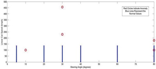
FIGURE 12 Anomalous values.

FURTHER WORK AND RESEARCH

Thus, a polynomial regression network was able to learn the best control values for the wheels to stabilize the vehicle in a quick amount of time. Thus, such models, when implemented in the large scale, can be improved further with precise accounts of car mechanics. Anomalies in the assistive system were also detected, thus preventing wrong control by the intelligent system. Such models not apply only to electric cars, but also to robotic driving systems for precise control of their movement.

Machine learning and artificial intelligence have interesting opportunities in almost all fields in the world today. In the automobile industry, they can revolutionize user driving experience. The driver assistive system opens new avenues for smart driving systems. Further integration of intelligent driving systems with biosensors for measuring driver attention and car position and proximity sensors can form an accident-proof and intelligent car that is able to make its own decisions.

ACKNOWLEDGMENTS

We thank SRM University for providing us a learning and productive platform for testing of our project. We also wish to deeply thank Prof. Andrew N.G, Associate Professor at Stanford University for his online course on Machine Learning. Heartiest thanks for line drawings to Ritendra Chakrabarty, undergraduate student of Electrical Engineering at SRM University.

REFERENCES

- Chandola, V., A. Banerjee, and V. Kumar. 2007. Anomaly detection: A survey. ACM Computing Surveys 41(3).
- Fu, C., Hoseinnezhad, R, Watkins, S and Nakahie Jazar, G. 2012. ‘Electronic differential design for vehicle side-slip control’, in Van-Minh Chau, Xuan-Man Nguyen, Nguyen-Vu Truong (ed.) Proceedings of the 2012 International Conference on Control, Automation and Information Sciences, United States, 26–29 November 2012, pp. 306–310.
- Haddoun, A., Benbouzid, M. E. H., Diallo, D., Abdessemed, R., Ghouili, J., and Srairi, K. (2007, May). Analysis, modeling and neural network traction control of an electric vehicle without differential gears. In Electric Machines & Drives Conference, 2007. IEMDC’07. IEEE International (Vol. 1, pp. 854–859). IEEE.
- Hartani, K., M. Bourahla, Y. Miloud, and M. Sekkour. 2008. Direct torque control of an electronic differential for electric vehicle with separate wheel drives. Journal of Automation & Systems Engineering (JASE) 2(2).
- Hartani, K., M. Bourahla, Y. Miloud, and M. Sekkour. 2009. Electronic differential with direct torque fuzzy control for vehicle propulsion system. Turkish Journal of Electrical Engineering & Computer Sciences 17(1).
- Ng, A. 2013a. Large scale machine learning. Machine learning, No. 17.
- Ng, A. 2013b. Advice for applying machine learning, Machine learning, No. 10.
- Ng, A. 2013c. Anomaly detection, Machine learning, No. 15.
- Smith, A. E., and A. K. Mason. 1996. Cost estimation predictive modeling: Regression versus neural network. The Engineering Economist 42(2):137–161.
- Vitols, K., and I. Galkin. 2012. Analysis of electronic differential for electric kart. In Proceedings of the 15th international power electronics and motion control conference. IEEE.
- Zhai, L., and S. Dong. 2011. Electronic differential speed steering control for four in-wheel motors independent drive vehicle. In Proceedings of the 8th world congress on intelligent control and automation. IEEE.
- Zhao,Y. E., J. W. Zhang, and X. Q. Guan. 2009. Modelling and simulation of electronic differential system for electric vehicle with two-motor-wheel-drive. In Intelligent vehicles symposium, 1209–1214. IEEE.