A Novel Crossing Minimization Ranking Method

Abstract

The ranking problem consists of comparing a collection of observations and deciding which one is “better.” An observation can consist of multiple attributes, multiple data types, and different orders of preference. Due to diverse practical applications, the ranking problem has been receiving attention in the domain of machine learning and statistics, some of those applications being webpage ranking, gene ranking, pesticide risk assessment, credit-risk screening, etc. In this article, we will present and discuss a novel and fast clustering-based algorithmic ranking technique and provide necessary theoretical working. The proposed technique utilizes the interrelationships among the observations to perform ranking and is based on the crossing minimization paradigm from the domain of VLSI chip design. Using laboratory ranking results as a reference, we compare the algorithmic ranking of the proposed technique and two traditional ranking techniques: the Hasse Diagram Technique (HDT) and the Hierarchical Clustering (HC) technique. The results demonstrate that our technique generates better rankings compared to the traditional ranking techniques and closely matches the laboratory results that took days of work.

INTRODUCTION

Ranking is an association between a set of observations or items. For any two observations, the first observation or item is ranked either lower than, higher than, or equal to the second item or observation. In the ranking problem, two different observations are compared to decide which one is “better.” In mathematics, this is known as a total preorder or a weak order of objects. Because two different objects can have the same ranking, ranking may not necessarily be a total order of objects. But, ranking itself is totally ordered. In ranking, a real-valued function assigns scores to objects; the scores themselves are not important, what matters is the objects’ relative rankings induced by those scores. Although the score-based sorting approach can be used for ranking, such as Okapi BM25 or Multilevel Sorting (MLS), we note that sorting is impervious to the underlying interrelationships between different items/observations with reference to their attributes.

The ranking problem has various practical applications including (but not limited to) problems related to document retrieval, credit-risk screening, selecting best items on an online auction site, and the list goes on. Therefore, the ranking problem has received increasing interest in both the statistical and the machine learning literature (Freund et al. 2003; Cortes and Mohri 2004; Agarwal et al. 2005; Usunier et al. 2005; Cao et al. 2006; Cossock and Zhang 2006; Rudin 2006; and Vittaut and Gallinari 2006). For example, in a document-retrieval application, the interest is in comparing documents by their degree of relevance for a particular search or topic instead of just classifying them as being relevant or not. Banks collect and manage large databases containing the sociodemographic and credit history data of their clients and use a ranking system that aims at indicating reliability. Similarly, in computational biology, one wants to rank genes according to their relevance to some disease. For an online auction site, one generally wants to pay less and buy from reputable sellers; in other words, some parameters or attributes are desired to have higher value and others lower value. The question is, how can this be decided automatically when there are dozens of attributes? Thus, ranking problems are mathematically distinct from both regression and classification and cannot be analyzed by simply using existing solutions for these problems.

Applications of Ranking

Ranking can provide an overall view of a certain set of objects or clusters, which is beneficial in comprehending the most important information in a short time. Some practical applications of ranking are as follows:

• Webpage ranking: There are many practical applications of ranking in the context of webpage search: (1) displaying ranked pages for a search query; (2) query refinement and spelling correction, in other words, displaying ranked suggestions and candidate corrections; (3) webpage summary, or displaying ranked sentence segments that also have related applications in order to select advertisements to display with a query result; (4) crawling/indexing a website based on page ranking, that is, identifying which page to crawl first and which pages to keep in the index based on their priority/quality.

• Gene ranking: Gene expression data is like a gold mine from which valuable knowledge can be extracted. However, a major problem in mining gene expression data is the existence of a large number of irrelevant or noisy genes along with the informative genes. Therefore, prior to using gene expression data, feature selection (also termed gene selection) is often performed to remove irrelevant and noisy genes. Depending on the selection criterion, feature selection techniques can be divided into two types: set-based feature selection and ranking-based feature selection. In ranking-based feature selection, or feature ranking, features are usually evaluated on an individual basis. Feature ranking might be preferred by biological researchers because it is simple and the selected genes can be verified individually (Yang and Mao 2010).

• Personalized ranking: Social networks and online communities have become one of the most successful collaborative platforms in the history of the Web. One of the keys to the success of e-commerce and social-network-related practical applications is personalized ranking capability for search, recommendation, and question answering. These practical applications require ranking a set of multiattribute items in order to help a user find the item of best choice among all available items. Consider someone interested in buying an iPad 5 on eBay. There are many sellers having different reputations selling iPad 5 at different prices. A buyer expects eBay to provide a personalized ranking of all sellers with high ranking accuracy. Meaning, given a user and a set of multiattribute items from which the user needs to select the best choice, the best choice is to be ranked as high as possible in the ranking list. More precisely, the best choice for the buyer is the seller from whom the buyer will purchase an iPad after an exhaustive search from all available sellers.

• Pesticide risk assessment: The availability of a very large number of pesticides, chemicals, and substances makes their ranking a challenging task, because (1) how do we find out quickly which pesticides are hazardous? A risk assessment of pesticides requires many time-consuming and expensive tests; and (2) with which pesticides or chemicals should we begin? According to Yazgan and Tanik (2004), pesticides with similar and/or identical agricultural characteristics have different behaviors in terms of their environmental impact. Therefore, it is possible to choose a substitute less harmful to the environment and obtain the same efficacy. Thus, according to Newman (1995), there is a need for fast ranking in order to provide a good starting point or operating sequence for the necessary tests and investigations. Thus, the decision on selection of the appropriate pesticide requires a ranking system; this is the main application of the proposed technique (PT) that we will discuss in this article.

Types of Ranking

Per Fürnkranz and Hüllermeier (2011), the three main types of rankings are as follows:

1. Label ranking: In label ranking, the model has an instance space X = {x_i} and a finite set of labels Y = {y_i|i = 1, 2, …, k}. The preference information is given in the form y_i > _xy_j indicating that instance x shows preference in y_i rather than y_j. A set of preference information is used as training data in the model. The task of this model is to find a preference ranking among the labels for any instance.

2. Instance ranking: Instance ranking also has the instance space X and label set Y. In this task, labels are defined to have a fixed order y₁ > y₂ > … y_k, and each instance x_l is associated with a label y_l. Given a set of instances as training data, the goal is to find the ranking order for a new set of instances.

3. Object ranking: Object ranking is similar to instance ranking except that no labels are associated with instances. Given a set of pairwise preference information in the form x_i > x_j, the model should find a ranking order among instances.

Our work falls under the domain of object ranking. Note that our work is not about learning to rank or training a ranking model using supervised learning for information presentation (Jiang, Lee, and Lee 2011); in our work we use unsupervised learning—clustering—for ranking.

CROSSING MINIMIZATION

Crossing minimization is among the oldest and most fundamental problems arising in the area of automatic graph drawing and very large scale integration (VLSI) design and has been studied in graph theory for many decades. Its two variants, the one layer (or one partition) and two layers (or two partitions) are NP-complete problems (Garey and Johnson 1983).

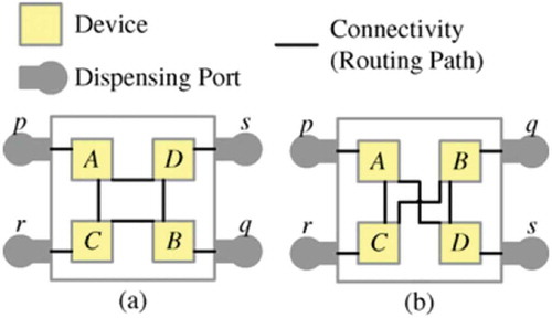
In VLSI Integrated Circuit (IC) design, placement of transistors or terminals or devices has a key role with reference to area, resistance, wire length, and other objectives. Thus, it is necessary to consider routing path crossings during placement because the placement topology determines the minimum possible number of path crossings introduced. Consider the design illustrated in Figure 1 with four devices, four dispensing ports, and connectivity (required routing paths) among them. The placement topology in Figure 1(a) results in crossing-free routing paths, whereas the placement topology in Figure 1(b) will always have at least one crossing among the paths no matter how these paths are routed.

FIGURE 1 Illustration of the fact that the minimum number of routing path crossings is determined by the placement topology, and this minimum number cannot be reduced by routing or by compactness changes. (a) Placement topology with zero routing path crossing. (b) Different placement topology that implements the same design in (a) but has at least one routing path crossing (Lin and Chang 2011). © 2011 IEEE. Reprinted, with permission, from IEEE Transactions.

Thus, the crossing problem on bipartite graphs can be illustrated with Figure 2. Given a bipartite graph G_B (two-partitioned network) with: (1) two partitions of vertices with V = {v₁, v₂, …, v_|V|} for the TOP partition and U = {u₁, u₂, …, u_|U|} for the bottom (BOT) partition; (2) a set of edges E ⊆ V × U; and (3) the permutation of vertices in the TOP and BOT (i.e., π_TOP and π_BOT); the crossing problem asks us to find the ordering or permutation of the vertices in the TOP and BOT that minimizes the number of crossings between the edges in E. Figure 2 (a and b) shows two possible orderings that lead to different numbers of crossings.

FIGURE 2 Crossing problem on bipartite graphs. (a) Ordering with four crossings (shown by dotted circles); (b) different ordering without crossings.

There are basically three types of crossing minimization heuristics (CMH). The first, more classical, type does not count the crossings and, as a result, these CMH are very fast and yet give good results. Examples include the barycenter heuristic (BCH) proposed by Sugiyama, Tagawa, and Toda (1981) and the median heuristic (MH) proposed by Eades and Wormald (1986). Other than the classical heuristics, there are also a number of other CMH that permute the vertices in the two bipartitions by counting crossings. These CMH, however, have a higher time complexity, such as simulated annealing by May and Szkatula (1988), genetic algorithms by Mäkinen and Siirtola (2005), Tabu search by Laguna, Martí, and Valls (1997), branch-and-bound (Valls, Martí, and Lino 1996; Jünger and Mutzel 1997) and stochastic hill-climbing by Newton, Sýkora, and Vrt’o (2002). Finally, there are the so-called metaheuristics that make use of classical heuristics to generate the initial arrangement of vertices and then improve on it by using other heuristics.

This work pursues the classical approach in which the ordering of vertices is repeated a constant number of times; therefore, the heuristic must be efficient (i.e., of lower time complexity; detailed time complexity analysis is in the analysis section).

LINEAR ARRANGEMENT AND RANK AGGREGATION

There are subtle differences w.r.t. crossing minimization among the problem considered in this study and the two problems of linear arrangement and rank aggregation. Therefore, before proceeding with the main work, we take a quick look at the focus of this article w.r.t. these three problems. The rank aggregation problem is to combine k different, completely ranked lists on the same set of n elements into a single ranking that best describes the preferences expressed in the given k lists. According to Biedl, Brandenburg, and Deng (2006), solutions to the crossing minimization problem can be used to solve the rank aggregation problem with applications in metasearch and spam reduction on the Web. Our work, however, involves ranking rows/observations or items in a table, which are unlikely to have a priori ranking; furthermore, our work does not involve combining ranked lists.

Per Gutin et al. (2007), a linear arrangement (LA) is an assignment of distinct integers to the vertices of a graph. The cost of an LA is the sum of edge lengths of the graph such that an edge length is defined as the absolute value of the difference of the integers assigned to its ends. Determining if a given graph has a minimum LA (MinLA) of cost bounded by a given integer is a classical NP-complete problem. Per Shahrokhi et al. (2001), crossing minimization can be used to solve the LA problem with accuracy guarantee of O(log n) from the optimal value, but MinLA is about mapping the vertices of a graph on an integer line with absolute minimum edge lengths instead of ranking those vertices, which is the focus of our work.

KEY CONTRIBUTIONS

The key contributions of our work are as follows:

1. A generic clustering-based ranking technique, i.e., proposed technique (PT) based on the crossing minimization paradigm, with theoretical treatment given for the concept

2. Comparison of the PT’s ranking results with results of the lab work of Chakraborty et al. (2011) and the comparison of these results with results of traditional ranking techniques: the Hasse diagram technique (HDT) and the hierarchical clustering (HC) Technique; all results quantified using an established distance metric (Gutin et al. 2007) and R² value

3. Proof of the low time complexity and scalability of the PT compared to the traditional ranking techniques considered

4. Demonstration that PT generates clean visualizations with minimal or no subjectivity, compared to the traditional techniques

RANKING TECHNIQUES

In this section, we will first give a formal overview of ranking, we will then discuss how clustering can be used for ranking, and we will establish the relationship between ranking and crossing minimization, which will be followed by ranking using HDT and HC.

In a ranking method (Restrepo et al. 2008), members of a set G consisting of objects a, b, … are ranked based on their different properties or attributes, i.e., q₁, q₂, …, q_i. Consider a set of chemicals G = {a, b, c, d, e, f, g} described and shown in the data matrix of Figure 3. A linear ranking is obtained if only one property q_i is considered; for example, linear ranking of Figure 1(a) is achieved if only q₁ is considered, and Figure 1(b) if only q₂ is considered. Because the descriptor q₂ of a is equal to that of b [q₂(a) = q₂(b)] and the same is true for e and g, i.e., [q₂(e) = q₂(g)], each of these pairs is equivalent in the ranking of Figure 1(b), that is, a ˜ b and e ˜ g. If q₁ and q₂ are hazardous properties of chemicals whose values increase with the extent of adverse impact, ranking of Figure 3(a) shows that a is the “most hazardous” substance, whereas from the ranking of Figure 3(b), it is d. In real life, the objects to be ranked are described by several descriptors or properties, all of which have to be considered simultaneously.

FIGURE 3 Data matrix of seven chemicals described by q₁ and q₂; rankings according to (a) q₁ and (b) q₂; (c) ranking due to a weighted combination of q₁ and q₂ (aggregation) (Restrepo et al. 2008).

According to Davis, Swanson, and Jones (1994), many ranking methods perform a weighted combination of descriptors to yield a new super descriptor. For example, the utility function described by Seip (1994), Γ(x), is calculated for each object x by assigning a weight gi to each descriptor qi as in Equation (1).

(1)

If equal priorities are assigned to q₁ and q₂, Γ(x) values can be depicted in a linear order as shown in Figure 3(c). Although all descriptors are simultaneously used, establishing the weight of each descriptor is still subjective.

Ranking by Clustering

Cluster analysis or clustering is the task of assigning a set of objects into groups or classes (called clusters) such that the objects in the same class or cluster are more similar (in one sense or another) compared to objects in other clusters or classes. For example, clustering can be used for antimoney-laundering by discovering abnormal patterns in a large number of bank transactions. Classification is a data mining technique that assigns objects in a collection to known target categories. The goal of classification is to accurately predict the target group for each case in the data. For example, a classification model could be used to identify loan applicants as high, medium, or low credit risks. Per www.oracle.com, classifications are discrete and do not imply order, therefore, classifications do not seem to be suitable for ranking.

In Cai et al. (2010) simultaneous clustering and ranking has been discussed. Figure 4 shows three approaches to ranking. Figure 4(a) shows traditional ranking; that is, there is no significant supporting technique or methodology for preranking. Figure 4(b) is a recent ranking methodology that uses clustering for preranking, also called cluster-based ranking and discussed by Jiang, Lee, and Lee (2011), Liu and Croft (2004), Giannopoulos et al. (2011), Wan and Yang (2006), Park et al. (2007), Wang, Li, et al. (2008), Wang, Zhu, et al. (2008) and Qazvinian and Radev (2008). This approach consists of applying a clustering algorithm to first obtain a cluster and then ranking the results within each cluster or exploring the interaction among cluster members. However, despite incorporating cluster-level information in ranking, clustering and ranking are regarded as two independent processes. In this study, we will follow the approach of Figure 4(c) and adopted by Cai et al. (2010), Giannopoulos et al. (2011), Gulli (2006), Sun et al. (2009), and Kluger et al. (2003); i.e., ranking and clustering have not only a mutual reinforcement property, but the quality of both can be improved when both are mutually enhanced.

FIGURE 4 Ranking and clustering (Cai et al. 2010).

In Gulli (2006), it was demonstrated that both clustering and ranking have a mutual reinforcement property. This property can be exploited to boost the precision of both methodologies. In one direction, a good ranking strategy can provide a valuable base of information for clustering in a dynamically organized hierarchy. In the other direction, a good cluster strategy can provide a valuable base for altering the rank of the retrieved answer set by emphasizing hidden knowledge meanings. The research by Gulli (2006) pointed out that the relationship between clustering and ranking produces mutual benefits; the better the clustering built on-the-fly, the better the results of the ranking algorithms. Clustering and ranking methodologies are, thus, closely related.

Sun et al. (2009) showed, on the one hand, that ranking evaluates objects of information based on some ranking function that mathematically demonstrates characteristics of objects. With such functions, any two objects of the same type can be compared, either qualitatively or quantitatively, in a partial order. On the other hand, clustering groups objects based on a certain proximity measure so that similar objects are in the same cluster and dissimilar ones are in different clusters. Moreover, assigning ranks to objects often leads to better understanding of each cluster. Obviously, good clusters promote good ranking.

In Kluger et al. (2003), a spectral biclustering method has been developed based on the observation that checkerboard structures in matrices of expression data can be found in eigenvectors corresponding to characteristic expression patterns across genes or conditions. The clustering method of Kluger et al. (2003) not only divides the genes into clusters, it also ranks the degree of membership of genes (and conditions) to the respective cluster according to the actual values in the partitioning-sorted eigenvectors. Such rankings may also be useful for studying ranking of patients within a disease cluster, in relation to prognosis.

The idea of “learning to rank” has recently become popular. The idea consists of using machine learning techniques to perform ranking from the given training data. The different “learning to rank” approaches can be divided into three categories: pointwise, pairwise, and listwise (Jiang, Lee, and Lee 2011), and our approach is closely related to pointwise. In the pointwise approach, the ranking problem is transformed into a classification problem. In our approach, instead of using classification, we use clustering. Thus, our approach is aligned with the approach of Giannopoulos et al. (2011), in which ranking models are clustered for historic queries according to user behavior and intent. Subsequently, each cluster is finally represented by a single ranking model. Optimally, the clustering and the ranking models are optimized jointly (Giannopoulos et al. 2011).

Ranking and Crossing Minimization

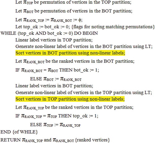
In this section we will discuss how ranking and crossing minimization are related. Consider Figure 5, which shows the pseudocode for a generic classical CMH. Here, LT is the set of techniques for classical CMH that don’t count the crossings. Those classical techniques use average and median values (i.e., BCH and MH, respectively, as mentioned in “Crossing Minimization.”

FIGURE 5 Pseudocode for a generic CMH using LT {BC, MH}.

Consider Figure 6, which shows a bipartite graph G_B with N vertices in the TOP partition with permutation π_TOP shown by a dotted boundary; π_BOT is defined similarly. The vertex set V in TOP is connected to the vertex set U in the BOT partition with connectivity defined by the INTERCONNECTION between the two partitions; here, the degree of vertex v_i is d(v_i).

FIGURE 6 Ranking by linear and nonlinear labeling of vertices in TOP and BOT partitions of G_B.

Let linear labeling be done first for the vertices in the TOP partition (shown by arrow), i.e., ℓ_i, ℓ_{i + 1}, ℓ_{i + 2}, … ℓ_{i + N − 1} such that ℓ_i < ℓ_{i + 1} < ℓ_{i + 2} … < ℓ_{i + N − 1} and by definition ℓ_{i + 1} − ℓ_i = 1, note that the value of ℓ₁ = 1. Linearly labeling the vertices in TOP and performing LT per the INTERCONNECTION generates the labels for the vertices in BOT. Let the labels generated for the BOT be denoted by ξ and assigned to the vertices as ξ_i, ξ_{i + 1}, ξ_{i + 2}, … ξ_{i + N − 1}. The relationship between the vertex labels in the BOT partition cannot be predicted, therefore we call it nonlinear labeling, i.e., ξ_{i + 1} − ξ_i {− ve, 0, + ve}.

Although it is difficult to predict the values of the labels in the BOT partition when the vertices in the TOP are labeled linearly, the vertices in the TOP partition that are in close proximity will always have similar label values, and their adjacent vertices in the BOT partition will have similar label values by virtue of using any one of the two considered techniques in LT. Subsequently, sorting labels ξ results in ranking of vertices in BOT with crossings reduced. Let the new ranked permutation of vertices in BOT be π_{RANK_BOT}, note that after ranking, ξ_{i + 1} − ξ_i {0, +}. If π_{RANK_BOT} and π_BOT are the same, it means no further improvement is needed for BOT.

However, ranking cannot be terminated yet because there might still be room for improvement in the TOP partition. Therefore, linear labeling of the vertices in the BOT partition ℓ_i, ℓ_{i + 1}, ℓ_{i + 2}, and ℓ_{i + N − 1} such that ℓ_i < ℓ_{i + 1} < ℓ_{i + 2} and < ℓ_{i + N − 1} and by definition ℓ_{i + 1} − ℓ_i = 1. Repeating the above process will inductively rank the vertices in the TOP partition with the ranked permutation of vertices in the TOP being π_{RANK_TOP}. If π_{RANK_TOP} and π_TOP are the same, no further improvement is necessary for TOP. However, ranking cannot be terminated yet, because there might still be room for improvement in the BOT if π_{RANK_BOT} and π_BOT were not the same. If both partitions cannot be improved further, then stop, because the vertices in both partitions are now ranked. Thus, we see that the classical CMH discussed here do not directly perform crossing minimization; actually, these CMH do not count the crossings, instead it is the ranking of nonlinear labeled vertices (corresponding step highlighted in Figure 4) that results in crossing minimization.

Observations:

1. Simply ranking the records by sorting w.r.t. their attribute values one by one or their weighted sum is impervious to the interrelationships between the records. These interrelationships are exploited by the attribute-based pairwise correlations between the records. This is subsequently used to create G_B, whose vertices with nonlinear labels generated by LT are ranked by sorting.

2. By altering the labeling process between the TOP and BOT partitions and sorting, the number of vertex positional changes decreases, until no further changes are made, i.e., π_{RANK_TOP} is the same as π_TOP, and π_{RANK_BOT} is the same as π_BOT, and ranking stops.

3. For the special case when the density of G_B is 100%, every nonlinear label value will be unique, ξ_{i + 1} − ξ_i = 1, vertices in both partitions will be already ranked, and INTERCONNECTION will act as a one-to-one mapping.

Ranking by the Hasse Diagram Technique (HDT)

The HDT is a mathematical method that allows assessing order or ranking relationships, such as in chemicals. In this section, we will briefly define ranking along with the discussion on the working of the HDT; a simple example will be used to explain the basic concepts. This section is based on the seminal study of Restrepo et al. (2008).

According to Brüggemann and Bartel (1999), in the HDT, two objects x and y, characterized by the descriptors q₁(x), q₂(x), …, q_i(x) and q₁(y), q₂(y), …, q_i(y), are compared in such a way that x is ranked higher than y (x ≥ y) if all of its descriptors are higher than those of y (q_i(x) > q_i(y) i), or if at least one descriptor is higher for x while all others are equal (j q_j(x) > q_j(y), q_i(x) = q_i(y) for all others). In this case, x and y are said to be comparable. If all descriptors of x and y are equal, both substances are equivalent (Brüggemann and Bartel 1999). Furthermore, if x ≥ y and y ≥ z, then x ≥ z. If one descriptor q_j fulfills q_j(x) < q_j(y) while the others are opposite (q_i(x) ≥ q_i(y)), then x and y are incomparable and are not ordered with respect to each other (Brüggemann and Bartel 1999). Two objects are said to have a “coverrelation” if they are comparable and when no third object is between. Such order relationships can be graphically presented as a Hasse diagram (HD), as shown in Figure 7.

FIGURE 7 Data matrix of seven chemicals described by q₁ and q₂; ranking according to Hasse diagram (Restrepo et al. 2008).

The rules for drawing an HD are given by Brüggemann and Patil (2010). Note that it is NP-complete to determine if a partial order with multiple sources and sinks can be drawn as a Hasse diagram with zero crossings (Garg and Tamassia 1995). All HD plots presented in this article are obtained using the software DART 2.05.¹

Per Trotter (2001), objects with lines in only the downward direction have the highest ranks (maximal objects); for example, a and d in Figure 7. However, objects with lines in only the upward direction have the lowest ranks and are called minimal objects (for example, b and g in Figure 7). The absence of a line between two objects means that they are incomparable. Per Brüggemann, Halfon, and Bücherl (1995), if there is a sequence of lines connecting them in the same direction, for example, f and b, they are comparable (f ≥ b), although no direct line is drawn between them because it is already contained in the path f ≥ c, c ≥ b. The data matrix (Figure 7) shows that f and b are comparable because q₁(b) < q₁(f) and q₂(b) < q₂(f). Objects a and c are incomparable because q₁(a) > q₁(c), but q₂(a) < q₂(c). Such pairs are recognized in HDT because there are no lines between them, or they are connected by lines not following the same direction, for example, b and g in Figure 7.

Ranking by Hierarchical Clustering (HC)

Generally, all hierarchical clustering heuristics begin with n clusters, where n is the number of elements or records. Subsequently, the two most similar clusters are combined to form n-1 clusters, i.e., the first item is ranked. In the next iteration, n-2 clusters are formed, i.e., two items are ranked; following the same logic, this process continues until we are left with only one cluster; that is, all items are ranked. In various hierarchical clustering heuristics, only the rules used to merge clusters differ. For example, in the “simple linkage” approach, clusters are merged by finding the minimum distance between one observation in one cluster and another observation in the second cluster. In the “furthest neighborhood” approach, the furthest distance between two observations is taken, whereas in the “average linkage” approach, the average distance among observations belonging to each cluster is considered, subsequently merging them with a minimum average distance among all pairs of observations in the respective clusters. In Ward’s (1963) method, the distance is the ANOVA sum of squares between the two clusters. Here, ANOVA stands for Analysis of Variance (ANOVA); the technique for testing hypotheses by testing the equality of two or more populations means by examining the variances of samples taken.

We consider the problem of clustering as falling under the general problem of finding similarity/dissimilarity between elements in a group. There are a number of similarity measures used to calculate the pairwise distance between the pairs of objects; some of those measures are Euclidean distance, standardized Euclidean distance, Minkowski distance, Chebychev distance, Mahalanobis distance, Hamming distance, and Jaccard distance, to name a few.

WHY RANK PESTICIDES?

It is well known that aside from their benefit to yield, pesticides are considered as an important source of pollutants. Conscious or unconscious use or abuse of pesticides leads to contamination of both water and agriculture land. Therefore, while selecting the most appropriate pesticide for application against a certain pest for a particular crop, it is critical to take into consideration the environmental as well as the agricultural impact of that pesticide. At the European level, legislation such as European Directive 67/548/EEC requires that, prior to using plant protection products, their risk assessment has to be performed. There is also the REACH (Registration, Authorisation and Restriction of Chemicals) project of the European Union, whose goal is to protect the environment.

Magnitude of the Problem

Pesticides can be harmful to humans and the environment. Therefore, it is logical to use only those pesticides that have little or no adverse human or environmental impact. However, this is a daunting task. For example, the National Pesticide Information Retrieval System² has a database with over 125,000 products. According to Brüggemann and Drescher-Kaden (2003) and Ahlers (1999), the list of chemicals available between 1971 and 1981 in the European Union EINECS list,³ consisted of 100,000 chemicals, with almost 1000 new chemicals entering the market yearly. More than 60 million substances are listed in the CAS Registry of the American Chemical Society.⁴ Due to the large number of chemicals used worldwide, it is almost impossible to develop a fully quantitative risk assessment system. Therefore, chemical or pesticide ranking systems can be used as a first step for screening pesticides in order to identify those requiring further analysis.

RELATED WORK

Different pesticide-ranking systems are in use today and have been proposed with respect to different objectives; clustering has also been used for ranking of pesticides (Restrepo et al. 2008; Kabak, Ulengin, and Onsel 2008; Restrepo and Brüggemann 2005). Details of some of the more frequently cited work follows.

In Restrepo et al. (2008), clustering was used for the environmental ranking of 40 refrigerants in order to assess the relative environmental hazard posed by them; the refrigerants included those used in the past, those presently used, and some proposed substitutes. Ranking was based on ozone depletion potential, global warming potential, and atmospheric lifetime and was achieved by applying the HDT. The refrigerants were divided into 13 classes based on the concept of dominance degree, a method for measuring order relationships among classes. Our work is similar to the work of Restrepo et al. (2008) in that we, too, use clustering; however, in our work we do not rank classes; instead we use the ranking within the classes identified by the PT.

In Crickmore et al. (1998), a method was presented for the ranking of 133 pesticidal crystals. The reason for the study was that earlier nomenclature based on insecticidal activity for the primary ranking criterion had become inconsistent because of many exceptions. HC was used with rank assigned to the crystals with respect to their position within the dendrogram/tree. The ranking was based on primary, secondary, and tertiary levels of ranks in the dendrogram tree, which roughly corresponded to the cluster boundaries. Our work is similar in principle because the ranking is based on clustering of similar pesticides using crossing minimization, with the added benefit that the cluster boundaries are automatically identified by the PT itself. As we will demonstrate in this article, the robustness of the PT methodology is evident from highly correlated pesticides being ranked close together, as in the case of the work by Crickmore et al. (1998). The dissimilarity of our work is that the PT does not deal with nomenclature.

In this study, we have adopted the approach of automatic attribute selection proposed by Abdullah and Hussain (2007), which enhances global visualization. The attributes identified and used in this work are similar to those used by other researchers such as McDaniel et al. (2006), Gramatica, Papa, and Francesca (2004), and Halfon et al. (1996). In the work of Gramatica, Papa, and Francesca (2004), different parameters were used for ranking pesticides, such as LD₅₀, vapor pressure (VP), Henry’s law constant (H), and organic carbon partition coefficient (Koc), along with other parameters such as water solubility (Kow), which have also been used to rank pesticides. In McDaniel et al. (2006), the parameters used for ranking pesticides are the amount of active ingredient and types of pesticides. In Halfon et al. (1996), HDT was used for ranking pesticides; one of the purposes of that study was the identification of the most important criteria for assessing the chemicals. For example, elimination of a criterion such as “usage” was found to affect the ranking more than the elimination of the criterion water solubility. This aspect is addressed in the PT when attribute selection is performed.

TABLE 1 Data Matrix with Actual and Sort-Based Values

			Actual Values					Sort Order
Serial	Common Name	Class	ai	MW	Kow	Solubility	LD50	ai_S	MW_S	Kow_S	Sol_S	LD50_S
1	Deltamethrin	Pyrethroid	100	505	4.6	0.002	128	18	19	11	1	9
2	Methomyl	Carbamate	40	162	2.38	57.9	17	15	1	4	22	3
3	Dimethoate	Organophosphate	40	229	5.95	2.5	150	13	4	15	13	10
4	Quinalophos	Phophorous	25	298	4.6	22	71	10	6	10	19	6
5	fenopropathrin	Pyrethroid	10	349	6	0.33	66	4	8	16	8	4
6	Triazophos	Organophosphate	40	313	23	35	82	14	7	22	21	8
7	Befenthrin	Pyrethroid	10	423	6	0.1	70	3	15	17	5	5
8	chlorpyrifos	Organophosphate	40	351	4.7	2	155	12	9	13	11	11
9	Cyhalothrin	Pyrethroid	2.5	450	7	2	79	1	18	21	12	7
10	Acetamiprid	Nicotinoid	20	223	6.27	2.95	417	7	3	19	14	15
11	Cypermethrin	Pyrethroid	380	416	6.6	0.01	250	21	13	20	3	12
12	imidicloprid	Nicotinoid	70	256	0.57	0.51	450	16	5	1	9	16
13	Profenofos	Organophosphate	500	374	3.1	20	358	22	11	8	18	13
14	Fenavalerate	Pyrethroid	20	420	4	0.02	451	6	14	9	4	17
15	Abamectin	Avermectin	18	873	2.56	7.8	10	5	22	5	16	2
16	Indoxacarb	Carbamate	150	528	4.6	0.2	730	19	20	12	6	18
17	Cyfluthrin	Pyrethroid	25	434	5.62	0.002	869	8	17	14	2	19
18	Thiamethoxam	Neonicotinoids	240	739	3	23	37.38	9	2	2	15	21
19	Spinosad	Spinosyn	4.5	434	6.18	1.5	960	20	21	7	20	22
20	Betacyfluthrin	Pyrethroid	4.5	434	6.18	1.5	960	2	16	18	10	20
21	Thiodicarb	Nicotinoid	80	354	1.4	19.1	386	17	10	3	17	14
22	Endosulfan	Cyclodiene organochlorine	35	407	2.95	0.32	10	11	12	6	7	1

Recently, a ranking and scoring method, PestScreen (Juraske et al. 2007), has been developed as a screening tool to provide a relative assessment of pesticide hazards to human health and the environment. Each hazard measure is scored, weighted, and combined with pesticide application data to provide an overall indicator of relative concern, PestScore. Unlike PestScreen, the objective of our work is not to establish the relative concern of pesticides based on hazards to human health, but an overall ranking that includes determining the pesticide’s effectiveness against pests by using data mining. For example, based on similar attribute values, different pesticides belong to the same Pyrethroid Class (Table 1); however, based on the clustering of those attributes, PT ranks those pesticides within, or in close proximity to, the pesticide class. Thus, PT attempts to use attribute values to get a holistic view of the interrelationships among the pesticides in order to rank them.

In McDaniel et al. (2006), a pesticide ranking system developed by the Department of Agriculture, Maryland, was discussed. The rank of a pesticide is estimated by conducting survey analysis; the data used consists of the amounts and types of pesticides applied by different sources (e.g., farm operators, certified private pesticide applicators, commercially licensed businesses, public agencies, and 1500 farmers). In Levitan (1997), several methods and techniques for indexing and ranking pesticides were discussed; most of those techniques are algebraic based, some center on addition, some techniques are based on assignment of weights to the attributes, some techniques are rule based, and others are decision based. However, these techniques are not holistic in the sense that they do not consider the interrelationships among the attributes as does our work; this will be explained in the next section.

The PT is based on the concept of similarity class, which is similar to the work of Restrepo and Brüggemann (2005) but different in application. Recognize that through the process of clustering, we also find that each cluster is a similarity class and objects belonging to a particular cluster have similar properties. Thus, by using CMH to perform clustering, the members in a similarity class are ordered based on their interclass similarity, which is based on the gradual transitions in the properties of the members within that cluster. The similarity classes collectively rank the entire dataset or data matrix, because clustering and ranking mutually reinforce each other Gulli (2006).

In Rosario et al. (2004), the problem of displaying nominal variables in a general-purpose visual exploration tool is discussed using numerical variables. The specific focus was (1) how to assign order and spacing among the nominal values, and (2) how to reduce the number of distinct values to display. Intradimension clustering or classing used in Rosario et al. (2004) is done using the traditional data mining technique of hierarchical clustering. Our work is different from Rosario et al. (2004) because it is not limited to visualization, which is limited by screen resolution, especially for parallel coordinates; this is not the case for the PT.

Abdullah and Hussain (2006) proposed the idea of data mining by crossing minimization and subsequently performed biclustering. In this study, we have used crossing minimization for ranking pesticides instead of identifying biclusters in the wine dataset (i.e., two completely different applications and problems considered). In Abdullah, Hussain, and Barnawi (2012), the pesticide usage practices of cotton farmers were considered with reference to the days of the week, using hierarchical cluste ring and data profiling. In this work, neither farming activities nor effect of weekdays were considered; instead, physiochemical properties of pesticides were considered and their toxicity ranking by crossing minimization (i.e., two completely different applications and problems considered).

MATERIALS AND METHODS

In this section, we will first give a summary of the real dataset considered; this will be followed by an explanation of the PT, then a discussion of the similarity in application of the proposed technique with the US EPA (Environment Protection Agency 2000) guidelines for pesticide risk assessment, and, finally, an overview of the metrics for quantifying ranking.

Pesticide Dataset

Although cotton covers 2.5% of the world’s cultivated land, it uses 16% of the world’s insecticides; more than any other single major crop (Environmental Justice Foundation and Pesticide Action Network-UK 2007). Per Wilson, Basinski, and Thomson (1972), the cotton crop is susceptible to attack by 96 worms and mite pests. Therefore, it is considered to be the world’s “dirtiest” crop due to the heavy usage of pesticides. In this work, we therefore consider those cotton pesticides that were frequently used by more than 1500 farmers in District Multan of Pakistan. The farmer pesticide-usage data was collected by the Directorate General of Pest Warning and Quality Control of Pesticides (DGPWQCP), Punjab. According to the expert opinion of the personnel of DGPWQCP, of the 22 pesticides considered, 14 attributes were shortlisted in relation to toxicity. From those 14 attributes, nine quantitative attributes were considered in this study. The attributes considered were NotSync (i.e., not synchronized), contact, systemic, toxicity, dose, percentage active ingredient (i.e., ai [grams/liter]), molecular weight (i.e., MW in grams), oil-water partition coefficient (Kow), water solubility (i.e., Solubility [grams/liter]) and Lethal Dose (i.e., LD₅₀). The dataset considered is given in Table 1.

An LD₅₀ is a standard measurement of acute toxicity that is stated in milligrams (mg) of pesticide per kilogram (kg) of body weight. The lower the LD₅₀ dose, the more toxic the pesticide (www.epa.gov), thus, the LD₅₀ value is inversely proportional to the hazardous nature of the pesticide. According to Harris and Bowman (1981), insecticide toxicity in soil decreases with increasing solubility of the insecticides in water, thus, the solubility value is considered to be inversely proportional to the hazardous nature of the pesticide. According to Luttrell, Jederberg, and Still (2008), lower MW chemicals are less well absorbed than higher MW chemicals, thus, MW is directly proportional to the hazardous nature of the pesticide.

With regard to the actual attribute values, observe the diversity in their range of values as shown in Table 1. For example, the minimum value of MW is 162, whereas the maximum value of Kow is 7; similarly, the minimum value of solubility is 0.002, whereas the minimum value of LD₅₀ is 10. Thus, in order to have a common ground such that certain attributes do not numerically “overwhelm” other attributes, we need to transform the attribute values. However, instead of subjectively assigning values to attributes, resulting in an ad hoc approach, we define the derived attribute Sort Order based on sorting; in other words, an objective approach. We proceed by first sorting the attributes and subsequently using the sort order of that attribute value instead of the actual attribute value. More precisely, the N records for each attribute are sorted and then a sort order is assigned to each attribute value (from 1 to N), as shown in Table 1.

Table 1 shows the dataset used for ranking the pesticides; observe that the attributes CommonName and Class will not be used while ranking. It can be observed from Table 1 that the order of pesticides per their chemical class is fairly random. We have one set of derived attributes with suffix “_S” in Table 1. The “_S” suffix corresponds to the actual range of values replaced by a range of between 1 and 22. For example, the actual range of ai is between 2.5 and 500, but the range of ai_S is between 1 and 22.

Proposed Technique (PT)

The flowchart of the proposed technique is shown in Figure 8. The explanation of each step of the six-step technique is as follows:

Step 1: Automatic attributes selection. In real-life problems, the datasets have many attributes, or features. The work of John, Kohavi, and Pfleger (1994) suggests that the problem of feature subset selection involves finding a “good” set of features under some objective function. Some of those objectiv functions are prediction accuracy, structure size, and minimal use of input features. According to Yang and Honavar (1998), this presents us with a feature subset selection problem in the automated design of pattern classifiers. The problem refers to the task of automatically identifying and selecting a useful subset of attributes. This subset is used to represent patterns from a larger set of often mutually redundant, possibly irrelevant attributes with different associated measurement costs and/or risks. Thus, the objective of this step is to identify the attributes with interrelationships or “synergy” between them and subsequently use these attributes for ranking. Attributes selection is also useful when the data has a large number of attributes, because this results in reduction of attributes.

FIGURE 8 Flow chart of the proposed technique.

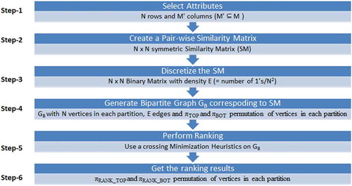
In performing automatic attribute selection on these nine attributes, using the technique of Abdullah and Hussain (2007), the last five attributes demonstrated interrelationships or synergy; hence, they were selected for the analysis performed in this study. These attributes can be considered to be representative of the pesticide characteristics and are similar to those used by other researchers for ranking pesticides, such as by Gramatica (2004).

Steps 2, 3, and 4: Generate and discretize similarity matrix, generate bipartite graph. Using the data matrix as input along with the selected attributes, a pairwise symmetric similarity matrix is generated using Pearson’s correlation. In order to reduce the complexity of the problem and to reduce the effect of noise, the similarity matrix is discretized. This discretization can be based on different criteria, such as mean or median or a certain percentile value. The discretized binary matrix can be considered to be the matrix data structure representation of a bipartite graph; hence, the corresponding bipartite graph G_B is generated. Observe that every vertex of G_B corresponds to a row of the data matrix and every edge corresponds to a strong interrelationship between the corresponding rows.

Step 5: Perform ranking. A CMH is used to perform ranking; this heuristic can be from different types of heuristics, as briefly described in the next section.

Step 6: Results. The permutation of vertices in a partition is the ranking of the corresponding rows of the data matrix.

Although the main focus of this study is to compare the ranking results of the proposed technique with HDT and HC, but without loss of generality, we also compare our ranking results with two additional ranking methods: the weighted algebraic sum (WAS) per Equation (1), and simple multilevel sorting (MLS). For the MLS, first, all records are sorted w.r.t. selected attribute A_i, then attribute A_j until all attributes are used.

Ranking and Pesticide Risk Assessment

The US EPA’s Supplementary Guidance for Risk Assessment (2000) proposes guidance on how to perform a risk assessment on a mixture of pesticides that act by a common mechanism. In Teuschler (2007), the US EPA guidance was expanded, and one method was added based on data for a single compound. The modified EPA guidance flowchart for single compounds is shown in Figure 9.

FIGURE 9 Flow chart of risk assessment method for single compound (Teuschler 2007).

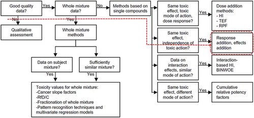
According to Bliss (1939), response addition assumes that the chemicals act by different modes of action and independently. Tolerance (or sensitivity) to one compound might or might not be correlated with tolerance to another. However, organisms most vulnerable or sensitive to chemical A may also be most vulnerable to chemical B (complete positive correlation). Similarly, organisms least vulnerable to chemical A may be least vulnerable to B (complete negative correlation), or the vulnerability to the two chemicals may be statistically independent.

In Figure 9, the dotted red line corresponds to the similarity in application of the proposed technique w.r.t. the modified EPA guidance flowchart for risk assessment from start to end. For example, we use quantitative data; the qualitative attributes such as class, formulation, and mode of action were not considered. Almost all the pesticides considered w.r.t. the practical example discussed in this article are used against the same organism (boll worms), and with different modes of action (contact and/or systemic). As a result of clustering the pairwise similarity matrix for the selected pesticides, pesticides with high positive correlation (say, pesticides A and B) get ranked together. If A and B are ranked together with high correlation, then the pests susceptible to pesticide A may also be susceptible to pesticide B. Thus making the PT conceptually similar to the pesticide assessment based on response addition for a single compound.

Quantification of Rank

A rank quantification metric is useful for quantifying the quality of a ranking. This quantification could be for the ranking done by a movie recommender system or ranking of images or ranking of webpages. Recommender systems typically use the historical access patterns or training samples provided by the users and the ranking is quantified based on the comparison with the training set. Image ranking is quantified based on the differences between the selected image and the reference image. Similarly, webpage ranking is quantified based on usage and related information generated by the interaction of the user with those pages. Thus, there is a reference, based on which the ranking is quantified. In our case, the reference is the pesticide ranking based on the laboratory study of Chakraborty, Korat, and Deb (2011).

More precisely, we quantify the rankings done in this work w.r.t. the laboratory results of Chakraborty, Korat, and Deb (2011) and the use of the cost formula for the MinLA problem. In the context of this work, the problem can be defined as follows: given an undirected and unweighted bipartite graph G_B with N vertices in each partition and a one-to-one function ψ: = V → [1, 2, 3, …, N], arrange the vertices of G_B on an integer line (ψ-label assignment), in order to minimize the following cost formula C:

(2)

PRACTICAL EXAMPLE

In this section, we will first give a brief outline of 3-day laboratory work for ranking toxicity of pesticides against useful insects (predators). We will then compare these results with the algorithmic ranking results of using five ranking techniques: PT, HDT, HC, WAS, and MLS. The comparison will be made using two established metrics: laboratory based and algorithmic based. Finally, we will do a time-complexity comparison of the algorithmic techniques considered.

Laboratory Ranking

Use of pesticides is one of the important components of Integrated Pest Management programs. However, insecticides/pesticides targeting insect pests in field conditions also damage the natural beneficial insects, that is, predators. The beneficial role of a particular biotic agent can be taken to suppress the pest population. Therefore, it is imperative to determine the safer chemicals in order to conserve the natural pest enemies in the field. Hence, in Chakraborty, Korat, and Deb (2011), the relative toxicity of 11 commonly used insecticides against the lacewing predator, Chrysoperla zastrowi silleni (Esben-Peterson), was assessed.

Eleven synthetic pesticides were evaluated for their ovicidal (i.e., egg) as well as larvicidal (i.e., larvae) action against C. zastrowi silleni. Each treatment was replicated thrice. In each replication there were ten eggs/larvae. The treated eggs were observed daily until all the eggs hatched in untreated control (up to 3 days). Mortality of larvae was recorded at 24, 48, and 72 hours after treatment and percent mortality was worked out. The laboratory ranking results are shown in Table 2.

TABLE 2 Comparison of the Laboratory and Algorithmic Toxicity Ranking of Five Pesticides against Lacewing Predator

			Algorithmic Rank
Lab Rank	Pesticides	Pesticide Serial	PT	HDT	HC	MLS	WAS
1	Endosulfan 0.07%	22	9	16	11	22	9
2	Imidacloprid 0.005%	12	6	20	20	7	14
3	Malathion 0.05%	–	Pesticide not in the list of 22 pesticides considered
4	Monocrotophos 0.036%	–	-do-
5	Fipronil 0.005%	–	-do-
6	Quinalphos 0.05%	–	-do-
7	Cypermethrin 0.015%	11	5	14	9	11	19
8	Indoxacarb 0.0075%	15	4	2	8	5	21
9	Fenvalerate 0.01%	14	3	17	4	6	5
10	Dichlorvos 0.05%	–	Pesticide not in the list of 22 pesticides considered
11	Dimethoate 0.03%	–	-do-

PT = Proposed Technique, HDT = Hasse Diagram Technique, HC = Hierarchical Clustering, WAS = Weighted Attribute Sum, MLS = Multilevel Sort, and Pesticide Serial is per Table 1.

Algorithmic Ranking

In this section, we will rank our 22-pesticide real dataset (Table 1) using three visual ranking techniques: PT, HDT, and HC. To generate the Hasse diagram, we will use the Decision Analysis by Ranking Techniques tool (DART 2.05). For HC we will use Hierarchical Clustering Explorer (HCE 3.5).⁵

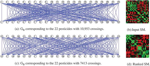
Figure 10 shows the unranked and ranked results of the PT using the 22-pesticide real dataset. Here, Figure 10(a) is the G_B corresponding to the 22 pesticides, whereas Figure 10(b) is the corresponding color-coded input similarity matrix. Here, red corresponds to negative correlations, green to positive correlations, and black indicates no correlation. Figure 10(c) shows the G_B corresponding to the ranked pesticides.

FIGURE 10 PT methodology results for 22-pesticide real dataset.

For the HDT based analysis, we will use the Hasse average rank generated by DART. The corresponding Hasse diagram is shown in Figure 11(a). 11(b) shows the HC, using five attributes, ranking results of 22 pesticides; clustering was performed via HCE 3.5 using average linkage and Euclidian distance.

FIGURE 11 (a) Hasse diagram results for 22-pesticide real dataset; (b) Hierarchical clustering technique results for 22-pesticide real dataset.

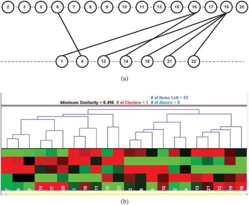
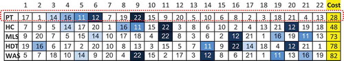
FIGURE 12 Comparison of the ranking by five techniques. Colored boxes are the pesticides considered by Chakraborty, Koran, and Deb (2011), their shades (dark to light) are the rankings done by Chakraborty, Koran, and Deb (2011), and Cost is the MinLA cost measure.

Comparison of Results

Of the 11 pesticides considered in Chakraborty, Korat, and Deb (2011), five are included in our study: Cypermethrin, Endosulfan, Fenvalerate, Imidacloprid, and Indoxacarb. These five pesticides are among the 22 pesticides that we have algorithmically ranked in this article, using the five techniques, PT, HDT, HC, WAS, and MLS. The results of the laboratory rank and the algorithmic rank of the five pesticides with reference to their toxicity for the green lacewing predator are given in Table 2.

We will now use two metrics to quantify the ranking w.r.t. Chakraborty, Korat, and Deb (2011), in other words, minimizing the cost function of the MinLA and comparing the rankings based on the R² value for the rankings line chart. For the MinLA comparison, we use the cost function of Equation (2). The MinLA cost of algorithmic ranking, using the five ranking techniques for the five pesticides common between our work and that of Chakraborty, Korat, and Deb (2011), is shown in Figure 12. Here, 1, 2 … 22 are the final rank positions.

From Figure 12 it can be clearly observed that the quality of PT ranking (shown by dotted boundary) w.r.t. Chakraborty, Korat, and Deb (2011) is significantly better than the other four techniques; actually the cost of PT is 41% less than the next-best traditional ranking technique, HC. This is basically due to the strong clustering properties of the PT compared with the other traditional ranking and clustering techniques considered in this article.

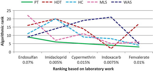
Figure 13 shows a line chart comparing the five algorithmic ranking techniques with reference to laboratory ranking of five pesticides. For ease of comprehension, the ranking results corresponding to the PT are shown by solid line, whereas the results for the other four techniques are shown by dotted lines. Observe the gradual transition in pesticide rank by the PT with reference to the laboratory ranking. No such gradual transition can be observed for the other four techniques.

FIGURE 13 Comparison of four ranking techniques with reference to the laboratory rank.

Discussion of Results

Because different assessment models/techniques take different approaches to incorporating indicators of exposure and assign greater weight to different aspects of the environment, different results are obtained. For example, in Levitan (1997), pesticides were ranked using three (Chems1, University of California Model [UC-Model], Environmental Impact Quotient Model [EIQ-Model]) pesticide assessment systems for establishing the “most hazardous” pesticide. Trifluralin was ranked at second position using Chems1, at seventh position using the UC-Model, and ranked not even in the top seven, using the EIQ model. The reason being that the three assessment systems emphasize different application areas: Chems1 emphasizes aquatic species; the UC-Model emphasizes human health, and EIQ emphasizes terrestrial species. The five ranking techniques considered in this article, however, have no such emphases, and are thus application-domain neutral.

Pesticide ranking will depend on a number of factors, some of those factors being the pesticides considered and the choice of attributes. Per the Pesticide Properties Database (PPDB),⁶ the pesticide properties are divided into three main groups: Environmental Fate (32 properties), Ecotoxicology (25 properties) and Human Health and Protection (13 properties) for a total of 70 properties. If we consider the subproperties, for example, soil degradation, the total properties increase further. Therefore, per the expert opinion of the personnel of DGPWQCP, for the 22 pesticides considered, 14 attributes were shortlisted relative to toxicity. As already discussed in this article, from those 14 attributes, five were automatically selected for ranking. Thus, the ranking generated in this study is a toxicity rank.

The comparison between the algorithmic rankings of the PT with the laboratory-based ranking can be precisely quantified using R² values for the line chart of Figure 13. The R² values between the algorithmic rank and laboratory rank for the five algorithmic ranking techniques being 0.92 for PT, 0.13 for HDT, 0.47 for HC, 0.59 for MLS, and 0.0006 for WAS. Based on the high R² value for the PT, a strong relationship is evident between the algorithmic rank of the PT with the laboratory rank.

The efficacy of pesticides is influenced by a number of factors, such as the dose, temperature of environment, relative humidity, development stage of the insect, to name a few. The 11 pesticides were ranked in the controlled laboratory environment therefore, many factors that influence the efficacy remain more or less constant. Whether field conditions or laboratory conditions, it is unlikely that the interrelationships among different pesticides and the synergy between their attributes will undergo a major change. Thus, the proposed technique with the selected attributes brings out the “natural” toxicity rank and order among the pesticides considered.

COMPARISON OF TIME COMPLEXITIES

In this section, we will perform a time-complexity analysis of the PT and the three other techniques, HC, HDT, and MLS.

PT Time Complexity

For PT, the worst-case time complexity occurs for the MH, because finding the median is intrinsically slow compared to finding the average or minimum (or maximum) value. To find the median of vertices in BOT, the worst-case linear time selection algorithm is used. The BC (barycenter) mean can be found in linear time, so is the minimum value for MinSort (MS). For each vertex i, the time to find the median will be O(d_i), where d_i is degree of vertex i.

Since , the time complexity to find the median of all vertices in BOT will be O(e). To ensure that the medians are always integers, the value is taken to be the median. Note that for the bigraph model being considered, the median will always be ≤ n, and by this property, counting sort is used to sort the median values in O(n) time. Thus, the time complexity of one iteration of the MH turns out to be O(max{e, n}) = O(e). The number of iterations taken to termination is O(1), resulting in time complexity O(e).

HC Time Complexity

The worst-case time complexity of complete-link hierarchical clustering is at most O(n² log n). One O(n² log n) algorithm to compute the n² distance metric and then sort the distances for each data point (overall time: O(n² log n)). After each merge iteration, the distance metric can be updated in O(n). We pick the next pair to merge by finding the smallest distance that is still eligible for merging. If we do this by traversing the n sorted lists of distances, then, by the end of clustering, we will have done n² traversal steps. Adding all this gives us O(n² log n). See also Aichholzer and Aurenhammer (1996) and Day and Edelsbrunner (1984).

HDT Time Complexity

The greedy knowledge acquisition procedure (GRAP) by Möbus and Seebold (2005) is for rapid prototyping of knowledge structures or spaces. By generating transitive closures greedily, GRAP controls the selection of nonredundant pairs, guarantees that the data comprise a partial order (surmise relation according to Doignon and Falmagne 1999), and generates the Hasse diagram of the surmise relation or the lattice of the concepts. On presentation of a pair (i, j) by GRAP, subjects have to select a judgment from a set of alternatives {“i causes/precedes j”, “i follows j”, “i neither causes/precedes nor follows j”}. In the best case, GRAP acquires the Hasse diagram in just one pass. In this case, the savings in judgments are (1−2/n)*100%, the judgment complexity is O(n), and the computational complexity is O(n³). In the worst case, GRAP needs n(n−1)/2 comparisons. The judgment complexity is O(n²) and the computational complexity stays O(n³).

Objects that are incomparable are considered as obstacles in obtaining a ranking (De Loof, De Baets, and De Meyer 2011). A popular approach that is not based on subjective assumptions and that overcomes this problem computes the average rank of each object in the linear extensions of the poset. A linear extension of a poset consists of the set of objects equipped with a linear order that is compatible with the partial order of the poset. Although algorithms to compute the average ranks are known (De Loof, De Meyer, and De Baets 2006; De Loof et al. 2008), because of their exponential nature, they are not suitable for posets with many incomparable objects.

Table 3 shows a comparison of time complexities of the four ranking techniques considered in this paper, observe the lowest time complexity of the proposed technique.

TABLE 3 Comparison of Time Complexities of the Four Ranking Techniques

No.	Technique	Time Complexity
1.	Clustering by Crossing Minimization	O(e)
2.	Hierarchical Clustering*	O(n^2 log n)
3.	Hasse Diagram Technique	O(n^3)
4.	MLS (Multilevel Sorting)	O(mn log n)

*http://nlp.stanford.edu/IR-book/completelink.html.

CONCLUSIONS AND FUTURE WORK

Ranking objects in a database is a challenging problem with diverse practical applications. In this article, we have demonstrated that clustering by crossing minimization can be used for ranking. The proposed technique (PT) exploits the interrelationships among the attribute of the records in order to quickly perform ranking. The results of the PT are better than those of the traditional ranking techniques. The efficiency of the PT is demonstrated by the fact that the ranking results closely match the laboratory ranking results. Thus, for assessment of chemicals/pesticides, the PT can be used as a first step to quickly screen pesticides in order to identify those requiring further analysis, thus saving time, money, and effort. More precisely, using the proposed algorithmic technique, in a few seconds we were able to closely replicate the ranking results that took 3 days of laboratory work.

The PT also generates clean visualizations that can help domain experts understand the ranking results. According to Brüggemann and Patil (2011), in general, Hasse diagrams lose their appealing charm when the number of objects is too large. The time complexity of the PT is linear in terms of the density of the discretized data matrix, resulting in a scalable ranking technique.

As part of future work, the PT could be used in other domains, such as webpage ranking, gene ranking, credit-risk assessment, and automatic recommendation systems, to name a few. It would also be interesting to compare the ranking techniques with reference to permutation and additive noise.

Funding

This work was funded by the Deanship of Scientific Research (DSR), King Abdulaziz University, Jeddah, under grant No. (611-004-D1433). The authors, therefore, acknowledge with thanks the DSR technical and financial support.

Notes

¹ http://www.talete.mi.it.

² http://www.ppis.ceris.purdue.edu.

³ http://chemicalwatch.com/927.

⁴ http://www.cas.org.

⁵ Available at http://www.cs.umd.edu/hcil/multi-cluster/.

⁶ http://www.eu-footprint.org/ppdb.html.

REFERENCES

- Abdullah, A., and A. Hussain. 2006. A new biclustering technique based on crossing minimization. Neurocomputing 69(16):1882 –1896.
- Abdullah, A., and A. Hussain. 2007. Using biclustering for automatic attribute selection to enhance global visualization. In Pixelization paradigm, 35 –47. Berlin, Heidelberg: Springer.
- Abdullah, A., A. Hussain, and A. Barnawi. 2012. Analysis of pesticide application practices using an intelligent agriculture decision support system ADSS. In Advances in brain inspired cognitive systems, 382 –391. Berlin, Heidelberg: Springer.
- Agarwal, S., T. Graepel, R. Herbrich, S. Har-Peled, and D. Roth. 2005. Generalization bounds for the area under the ROC curve. Journal of Machine Learning Research 6:393 –425.
- Ahlers, J. 1999. The EU existing chemicals regulation. Environmental Science and Pollution Research 6(3):127 –129.
- Aichholzer, O., and F. Aurenhammer. 1996. Classifying hyperplanes in hypercubes. SIAM Journal on Discrete Mathematics 9(2):225 –232.
- Biedl, T., F. J. Brandenburg, and X. Deng. 2006. Crossings and permutations. In Graph drawing, 1 –12. Berlin, Heidelberg: Springer.
- Bliss, C. I. 1939. The toxicity of poisons applied jointly. Annals of Applied Biology 26(3):585 –615.
- Brüggemann, R., and U. Drescher-Kaden. 2003. Introduction to the model-based assessment of environmental chemicals – Data Assessment, propagation, behavior, and effective evaluation. Berlin: Springer.
- Brüggemann, R., and H. G. Bartel. 1999. A theoretical concept to rank environmentally significant chemicals. Journal of Chemical Information and Computer Sciences 39(2):211 –217.
- Brüggemann, R., and G. P. Patil. 2010. Multicriteria prioritization and partial order in environmental sciences. Environmental and Ecological Statistics 17(4):383 –410.
- Brüggemann, R., and G. P. Patil. 2011. Ranking and prioritization for multi-indicator systems. Environmental and Ecological Statistics 5, New York, NY: Springer Science.
- Brüggemann, R., E. Halfon, and C. Bücherl. 1995. Theoretical base of the program “Hasse” (GSF, Technical Report, Bericht 20/95, Neuherberg, Germany).
- Cai, X., W. Li, Y. Ouyang, and H. Yan. 2010. Simultaneous ranking and clustering of sentences: A reinforcement approach to multi-document summarization. In Proceedings of the 23rd International Conference on Computational Linguistics, 134 –142. Cambridge, MA: The MIT Press/Association for Computational Linguistics.
- Cao, Y., J. Xu, T. Y. Liu, H. Li, Y. Huang, and H. W. Hon. 2006. Adapting ranking SVM to document retrieval. In Proceedings of the 29th annual international ACM SIGIR conference on research and development in information retrieval, 186 –193. New York, NY: ACM.
- Chakraborty, D., D. M. Korat, and S. Deb. 2011. Relative ovicidal and larvicidal toxicity of eleven insecticides to the green lacewing (Chrysoperla zastrowi silleni [Esben-Peterson]). In Insect pest management, A current scenario, ed. D, P. Ambrose, 107 –110. Palayamkottai, India: Entomology Research Unit, St. Xavier’s College.
- Cortes, C., and M. Mohri. 2004. AUC optimization vs. error rate minimization. Advances in Neural Information Processing Systems 16(16):313 –320.
- Cossock, D., and T. Zhang. 2006. Subset ranking using regression. In Learning theory, 605 –619. Berlin, Heidelberg: Springer.
- Crickmore, N., D. R. Zeigler, J. Feitelson, E. Schnepf, J. Van Rie, D. Lereclus,.. and D. H. Dean. 1998. Revision of the nomenclature for the Bacillus thuringiensis pesticidal crystal proteins. Microbiology and Molecular Biology Reviews 62(3):807 –813.
- Davis, G. A., M. Swanson, and S. Jones. 1994. Comparative evaluation of chemical ranking and scoring methodologies (Technical Report EPA Order No. 3N-3545-NAEX). Knoxville, TN: University of Tennessee Center for Clean Products and Clean Technologies for the United States Environmental Protection Agency.
- Day, W. H., and H. Edelsbrunner. 1984. Efficient algorithms for agglomerative hierarchical clustering methods. Journal of Classification 1(1):7 –24.
- De Loof, K., B. De Baets, and H. De Meyer. 2011. Approximation of average ranks in posets. Business Media Communications in Mathematical and in Computer Chemistry 66:219 –229.
- De Loof, K., B. De Baets, H. De Meyer, and R. Bruggemann. 2008. A hitchhikers guide to poset ranking. Combinatorial Chemistry and High Throughput Screening 11(9):734 –744.
- De Loof, K., H. De Meyer, and B. De Baets. 2006. Exploiting the lattice of ideals representation of a poset. Fundamenta Informaticae 71(2):309 –321.
- Doignon, J. P., and J. C. Falmagne. 1999. Knowledge spaces. Heidelberg: Springer.
- Eades, P., and N. Wormald. 1986. The median heuristic for drawing 2-layers networks (Technical Report 69). Brisbane, Australia: Department of Computer Science, University of Queensland.
- Environmental Justice Foundation and Pesticide Action Network-UK. 2007. The deadly chemicals in cotton. London: Author.
- Freund, Y., R. Iyer, R. E. Schapire, and Y. Singer. 2003. An efficient boosting algorithm for combining preferences. The Journal of Machine Learning Research 4:933 –969.
- Fürnkranz, J., and E. Hüllermeier. 2011. Preference learning: An introduction. In Preference learning, 1 –17. Berlin, Heidelberg: Springer.
- Garey, M. R., and D. S. Johnson. 1983. Crossing number is NP-complete. SIAM Journal on Algebraic Discrete Methods 4(3):312 –316.
- Garg, A., and R. Tamassia. 1995. On the computational complexity of upward and rectilinear planarity testing. In Graph drawing, 286 –297. Berlin, Heidelberg: Springer.
- Giannopoulos, G., U. Brefeld, T. Dalamagas, and T. Sellis. 2011. Learning to rank user intent. In Proceedings of the 20th ACM international conference on information and knowledge management, 195 –200. New York, NY: ACM.
- Gramatica, P., E. Papa, and B. Francesca. 2004. Ranking and classification of non-ionic organic pesticides for environmental distribution: A qsar approach. International Journal of Environmental Analytical Chemistry 84(1–3):65 –74.
- Gulli, A. 2006. On two web IR boosting tools: Clustering and ranking (Doctoral dissertation, PhD thesis, Dipartimento di Informatica, Universit ‘a degli Studi di Pisa, Italy).
- Gutin, G., A. Rafiey, S. Szeider, and A. Yeo. 2007. The linear arrangement problem parameterized above guaranteed value. Theory of Computing Systems 41(3):521 –538.
- Halfon, E., S. Galassi, R. Brüggemann, and A. Provini. 1996. Selection of priority properties to assess environmental hazard of pesticides. Chemosphere 33(8):1543 –1562.
- Harris, C. R., and B. T. Bowman. 1981. The relationship of insecticide solubility in water to toxicity in soil. Journal of Economic Entomology 74(2):210 –212.
- Jiang, J. Y., L. W. Lee, and S. J. Lee. 2011. RANKOM: A query-dependent ranking system for information retrieval. International Journal Of Innovative Computing Information And Control 7(12):6739 –6756.
- John, G. H., R. Kohavi, and K. Pfleger. 1994. Irrelevant features and the subset selection problem. In ICML ( vol. 94), 121 –129. New Brunswick, NJ: Morgan Kaufman.
- Jünger, M. and P. Mutzel. 1997. 2-layer straight-line crossing minimization: Performance of exact and heuristic algorithms. Journal of Graph Algorithms and Applications 1(1):1 –25.
- Juraske, R., A. Antón, F. Castells, and M. A. Huijbregts. 2007. PestScreen: A screening approach for scoring and ranking pesticides by their environmental and toxicological concern. Environment International 33(7):886 –893.
- Kabak, O., F. Ulengin, and S. Onsel. 2008. A new ranking methodology based on hierarchical cluster analysis. In 3rd international conference on intelligent systems and knowledge engineering, 2008 (ISKE 2008), 1:360 –365. IEEE.
- Kluger, Y., R. Basri, J. T. Chang, and M. Gerstein. 2003. Spectral biclustering of microarray data: Co-clustering genes and conditions. Genome Research 13:703 –716.
- Laguna, M., R. Martí, and V. Valls. 1997. Arc crossing minimization in hierarchical digraphs with tabu search. Computers and Operations Research 24(12):1175 –1186.
- Levitan, L. 1997. Pesticide impact assessment systems based on indexing or ranking pesticides by environmental impact. Revised Draft OECD Background Paper. Copenhagen, Denmark.
- Lin, C. Y., and Y. W. Chang. 2011. Cross-contamination aware design methodology for pin-constrained digital microfluidic biochips. IEEE Transactions on Computer-Aided Design of Integrated Circuits and Systems 30(6):817 –828.
- Liu, X., and W. B. Croft. 2004. Cluster-based retrieval using language models. In Proceedings of the 27th annual international ACM SIGIR conference on research and development in information retrieval, 186 –193. New York, NY: ACM.
- Luttrell, W. E., W. W. Jederberg, and K. R. Still, Eds. 2008. Toxicology principles for the industrial hygienist. Fairfax, VA: American industrial Hygiene Association.
- Mäkinen, E., and H. Siirtola. 2005. The barycenter heuristic and the reorderable matrix. Informatica Slovenia 29(3):357 –364.
- May, M., and K. Szkatula. 1988. On the bipartite crossing number. Control and Cybernetics 17(1):85 –97.
- McDaniel, J., H. Harris, R. Hyat, B. Yaylor, and G. Noguera. 2006. Maryland pesticides statistics for 2004, 1 –14. Maryland, USA: Department of Agriculture.
- Möbus, C., and H. Seebold. 2005. A greedy knowledge acquisition method for the rapid prototyping of Bayesian belief networks. In Artificial intelligence in education, 875 –877. Amsterdam, The Netherlands: IOS Press.
- Newman, A. 1995. Ranking pesticides by environmental impact. Environmental Science and Technology 29(7):324A –326A.
- Newton, M., O. Sýkora, and I. Vrt’o. 2002. Two new heuristics for two-sided bipartite graph drawing. In Graph drawing, 312 –319. Berlin, Heidelberg: Springer.
- Park, S., J. H. Lee, D. H. Kim, and C. M. Ahn. 2007. Multi-document summarization using weighted similarity between topic and clustering-based non-negative semantic feature. In Advances in Data and Web Management, 108 –115. Berlin, Heidelberg: Springer.
- Qazvinian, V., and D. R. Radev. 2008. Scientific paper summarization using citation summary networks. In Proceedings of the 22nd international conference on computational linguistics ( vol. 1), 689 –696. Manchester, UK: Association for Computational Linguistics.
- Restrepo, G., and R. Brüggemann. 2005. Ranking regions using cluster analysis, Hasse diagram technique and topology. In Proceedings of the 9th WSEAS international conference on computers, (ICCOMP’05), Article No. 36. Stevens Point, WI, USA: World Scientific and Engineering Academy and Society.
- Restrepo, G., M. Weckert, R. Brüggemann, S. Gerstmann, and H. Frank. 2008. Ranking of refrigerants. Environmental Science and Technology 42(8):2925 –2930.
- Rosario, G. E., E. A. Rundensteiner, D. C. Brown, M. O. Ward, and S. Huang. 2004. Mapping nominal values to numbers for effective visualization. Information Visualization 3(2):80 –95.
- Rudin, C. 2006. Ranking with a p-norm push. In Proceedings of COLT 2006, Lecture Notes in Computer Science 4005: 589 –604, ed. P. Auer and R. Meir. Berlin: Springer.
- Seip, K. L. 1994. Restoring water quality in the metal polluted Soerfjorden, Norway. Ocean and Coastal Management 22(1):19 –43.
- Shahrokhi, F., O. Sýkora, L. A. Székely, and I. Vrt’o. 2001. On bipartite drawings and the linear arrangement problem. SIAM Journal on Computing 30(6):1773 –1789.
- Sugiyama, K., S. Tagawa, and M. Toda. 1981. Methods for visual understanding of hierarchical system structures. IEEE Transactions on Systems, Man and Cybernetics 11(2):109 –125.
- Sun, Y., J. Han, P. Zhao, Z. Yin, H. Cheng, and T. Wu. 2009. Rankclus: Integrating clustering with ranking for heterogeneous information network analysis. In Proceedings of the 12th international conference on extending database technology: Advances in database technology, 565 –576. New York, NY: ACM.
- US Environmental Protection Agency, Risk Assessment Forum Technical Panel. 2000. Supplementary guidance for conducting health risk assessment of chemical mixtures. Washington, DC: Office of EPA/630/R–00/002.
- Teuschler, L. K. 2007. Deciding which chemical mixtures risk assessment methods work best for what mixtures. Toxicology and Applied Pharmacology 223(2):139 –147.
- Trotter, W. T. 2001. Combinatorics and partially ordered sets: Dimension theory ( Vol. 6). Baltimore, MD: Johns Hopkins University Press.
- Usunier, N., V. Truong, M. Amini, and P. Gallinari. 2005. Ranking with unlabeled data: A first study. In Proceedings of NIPS’05 workshop on learning to rank. Whistler, Canada: Massachusetts Institute of Technology.
- Valls, V., R. Martí, and P. Lino. 1996. A branch and bound algorithm for minimizing the number of crossing arcs in bipartite graphs. European Journal of Operational Research 90(2):303 –319.
- Vittaut, J. N., and P. Gallinari. 2006. Machine learning ranking for structured information retrieval. In Advances in information retrieval. Lecture Notes in Computer Science 3936:338 –349. Berlin: Springer.
- Wan, X., and J. Yang. 2006. Improved affinity graph based multi-document summarization. In Proceedings of the human language technology conference of the NAACL, Companion volume: Short papers, 181 –184. Madison, WI: Omnipress/Association for Computational Linguistics.
- Wang, D., T. Li, S. Zhu, and C. Ding. 2008. Multi-document summarization via sentence-level semantic analysis and symmetric matrix factorization. In Proceedings of the 31st annual international ACM SIGIR conference on research and development in information retrieval, 307 –314. New York, NY: ACM.
- Wang, D., S. Zhu, T. Li, Y. Chi, and Y. Gong. 2008. Integrating clustering and multi-document summarization to improve document understanding. In Proceedings of the 17th ACM conference on information and knowledge management, 1435 –1436. New York, NY: ACM.
- Ward, J. H. Jr. 1963. Hierarchical grouping to optimize an objective function. Journal of the American Statistical Association 58:236 –244.
- Wilson, A. G. L., J. J. Basinski, and N. J. Thomson. 1972. Pests, crop damage and control practices with irrigated cotton in a tropical environment. Cotton Growing Review 49(4):308 –334.
- Yang, F., and K. Z. Mao. 2010. Improving robustness of gene ranking by resampling and permutation based score correction and normalization. In IEEE International Conference on Bioinformatics and Biomedicine (BIBM ’10), 444 –449. IEEE.
- Yang, J., and V. Honavar. 1998. Feature subset selection using a genetic algorithm. In Feature extraction, construction and selection, International Series in Engineering and Computer Science 453:117 –136. New York, NY: Springer US.
- Yazgan, M., and A. Tanik. 2004. Transportation pathways of pesticides in two major watersheds of Istanbul, Turkey. Water Science and Technology 49(3):165 –172.