A Comparative Study: L1-Norm Vs. L2-Norm; Point-to-Point Vs. Point-to-Line Metric; Evolutionary Computation Vs. Gradient Search

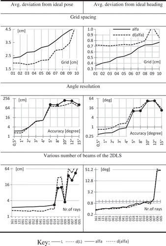
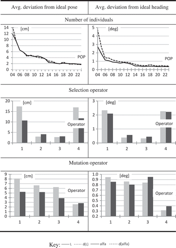
Abstract

The study presented in this article compares the two most frequently used regularizations in the robotics area: L1-norm and L2-norm, for navigation purposes of an autonomous mobile platform in an inner environment with use of the 2D laser scanner. Sensorial data in a real environment are very often burdened by a noise, which unfavorably affects the classification process. Presented results show behavior of all tested algorithms under conditions in which the sensorial data are loaded by common types of the noise: moving objects, quantizing noise, artificially added noise with different types of characteristics that correspond to potentially real conditions. Basic navigation mechanisms presented here use methods of robust statistics and modern evolutionary optimizers. The methods selected in this study represent the two different types of metrics, commonly called point-to-point and point-to-line. The navigation algorithm that uses L1-norm regularization integrates several different evolutionary algorithms that occupy a position of very efficient optimizers, which, at the same time, do not cut down limits of usability of the tested methods. Correct working parameters settings of all used pose estimators play a key role in the robot pose and heading estimation, therefore, this article is extended by a description of several important working parameters and the way to use them.

View correction statement:

Corrigendum

INTRODUCTION

In the area of autonomous mobile robotics, elementary spatial orientation is very important and a substantial part of all other control algorithms that are used not only in practice, but also at a research-laboratories level, depends on it. Most frequently, we can find various types of manipulators mainly in the automotive area, manufacturing, or mining industry. If a more advanced sensor is selected for navigation, for example, 2D laser scanner (2DLS), 3D laser scanner (3DLS), or video camera, in which feedback control of navigation success is provided by the identical sensorial apparatus, then the navigation algorithm requirements, and requirements to its robustness and accuracy, significantly increase as well as the computational demands. In the area of practical mobile robotic applications, another burden that can be removed only with difficulty is present: a noise originating from different sources and different, and very often not easily predictable, characteristics. The navigation is usually based on a model of an environment and a noise is approximated, for instance, by Gaussian noise. Basic navigation mechanisms must be capable of navigating even under such unfavorable conditions. Perfect noise modeling can be very difficult. Some authors solve this problem by not conducting noise modeling or noise filtration from the sensorial data, and they base the navigation on using the raw sensorial data (Cox 1991; Lu and Milios 1997; Weiss, Wetzler, and von Puttkamer 1994; Weiss and Puttkamer 1995; Thrun 2001; Nieto, Bailey, and Nebot 2006; Borrmann et al. 2008). The advantage of such an approach is the simplification of a control algorithm and also the fact that no useful data are lost by being accidentally removed in the filtration process. Based on the results presented in the articles mentioned, where in most cases the Besl and McKay (1992) method or its derivatives are used in navigation, it can be generally stated that such an approach is possible. Every navigation method has different accuracy, characteristics, and tolerance to a noise presence in sensorial data. The methods described in Cox (1991), Besl and McKay (1992), Lu and Milios (1997), and Diosi and Kleeman (2007), belong among the classic gradient optimizers. All of them provide good results; however, only in an area where the sensorial data are only subtly burdened by a noise. Nevertheless, all these algorithms are commonly used up to now as the basic navigation method; see, for instance, Kummerle et al. (2011).

The aim of this study is to provide more detailed findings of features of the two most often used navigation algorithms that can be described as L1-norm-based and L2-norm-based navigation algorithms in contrast to results presented in the article (Moreno et al. 2011). The article is divided into three parts: the first part focuses on the concept of localization and the detailed list of publications that use L1- or L2-norm regularization. Both tested methods are described as well. The second part deals with experiments in which the selected evolutionary algorithms (EA) are compared with classic L2-norm gradient algorithm (HillClimbing). The last chapter focuses on the discussion of working parameters selection.

RELATED WORK IN GENERAL

There are many approaches addressing the problem of localization. All of them can be easily classified into the following groups according to the way the map of the environment is interpreted: (1) metric maps, i.e., occupancy grid maps (Martin and Moravec 1996; Moravec and Elfes 1985; Elfes 1986; Moreno et al. 2009; Burgard et al. 1996; Skrzypczynski 2009), (2) feature-based maps (Diosi and Kleeman 2007) or topological maps (Lazanas and Latombe 1992; Sasaki et al. 2007; Remolina and Kuipers 2004), (3) hybrid methods Skrzypczynski (2009). With reference to the considerable number of articles covering this area of scientific research, it is possible to affirm that the individual groups are represented equally.

During the last decade, EAs have been used more often for simultaneous localization and mapping (SLAM) purposes. Although they prolong the implementation, at least they bring about the possibility to optimize the computation, maintaining the identical stability and resulting accuracy. The Monte Carlo optimizer (Metropolis and Ulam 1949) is frequently used together with probabilistic methods (Dellaert et al. 1999; Burgard et al. 1996; Fox, Burgard, and Thrun 1999). The simple genetic algorithm (SGA; Goldberg 1987, 1989; Holland 1992; Koza 1996; Whitley 1994) is the first purely evolutionary optimizer based on a sequential processing of various sorts of evolutionary operators: selection, crossover, mutation. In later years, a number of important optimizers were proposed, for example, differential evolution (DE; Storn 1996; Storn and Price 1997), particle swarm optimization (PSO; Kennedy and Eberhart 1995), whose contribution is, similarly to the case of SGA, restricted to a certain set of tasks that they are able to solve successfully. The EA scientific area is very extensive. There are myriads of different hybrid algorithms and other exotic derivatives of the aforementioned methods (aGA; Moravec 2012). One of the first articles in which the SGA utilization can be found for robot localization purposes was published by Ebner (1999). The island model genetic algorithm (IGA) was presented by Whitley, Rana, and Heckendorn (1998). The topic of distributed parallel SGA can be found also in earlier articles (Tanese 1989; Gorges-Schleuter 1991). The IGA has better results for linearly separated problems in comparison to SGA and is used, for instance, by Moreno et al. (2002). In Begum, Mann, and Gosine (2006a, 2006b) the IGA is used for SLAM, and in Begum, Mann, and Gosine (2008) it is possible to find a connection between the IGA and the fuzzy-logic system. “Evolutionary” SLAM is used also in Begum, Mann, and Gosine (2007). The DE for SLAM purposes is used in Moreno et al. (2009), as well. The basic algorithm uses the probability occupancy grid (Moravec and Elfes 1985; Fox et al. 1999). Kwok, Liu, and Dissanayake (2006) presented a study that compared the efficiency of the SGA, PSO, and AntSystem described in Dorigo (1992). The estimator that estimates the robot position and heading solves the three-dimensional (3D) optimization problem. Its disadvantage lies in the fact that it is necessary to use a large number of individuals and generations in the population. The chromosome is defined by the robot pose and heading as .

Currently, evolutionary algorithms are commonly used in many scientific areas. The SGA belongs among the oldest purely evolutionary algorithms. On the contrary, DE and PSO represent relatively young, but well-explored algorithms, so-called metaheuristics. Under certain conditions, all of them require run-time settings of the internal parameters, which can significantly extend the time needed for the computation. For some tasks, a priori settings are sufficient. For purposes of this comparative study, the mentioned metaheuristics were selected, namely: DE, PSO, SGA, and algorithm aGA. For all these algorithms, the fixed setting of all internal working parameters is used.

L1-NORM, L2-NORM RELATED WORK

In mathematics, so-called spaces are made of measurable functions whose th power is finitely integrable in . The space defined this way is a vector space with a finite number of dimensions. In such space the distance is defined as

(1)

These functional spaces are called Lebesgue spaces after French mathematician Henri Léon Lebesgue, and they were defined for the first time by Hungarian mathematician Marcel Reisz, as early as in 1910. From the practical point of view, in the area of robotics, most frequently metric spaces called and norms are used to express the self-similarity. The term provides one of the possibilities of how to express the self-similarity ratio of the surveyed course of two functions.

Over the several last decades, advantages and disadvantages of the methods that are based on the L1- or L2-norm were profusely described in technical literature of many scientific branches, for example, in medicine (Ding 2009), engineering (Parsopoulos et al. 2004), forecasting (Dielman 1986), statistics (Květoň 1987), computer sciences and image processing (Zhu et al. 2006; Fuchs 1984; Fu et al. 2006; Yan et al. 2009), robotics (Moreno et al. 2011). The L2-norm, also called least square method (LSM), represents a widely used computational scheme for estimation of parameters. However, the L1-norm (alias least absolute values, Manhattan norm, taxicab geometry) provides, in many practical applications, significantly better results in comparison to the L2-norm. Of course, this aspect depends on the type of the basic method used, and proofs can be found in many scientific articles, not only from theoretical, but also from applied researches (e.g., Fuchs 1984; Josselin and Ladiray 2001). The authors of one of the most recent articles are, for instance, Bektaş and Şişman (2010); or Fu et al. (2006), for example, proved that by using the minimization of mixed L2-L1- and L1-L1-norms in series-parallel ordering, significantly better results can be reached in comparison to the standalone L2- or L1-norm usage. Their article was focused on the filtration of a noise from video data (Fu et al. 2006). Very similar arrangement was selected also by Bilgiç (2010) to analyze the video data in search of moving pedestrians in video sequences. Useful information on the L1-L2-norm can be found also in Wilson (1978), Narula et al. (1999), and Narula and Wellington (1982). In general, there are no rules defining to what extent it is an advantage to use the algorithms based on the L1- or L2-norm to resolve a real problem. For example, in their article, Martin et al. (2009) proved that if the L1-L2-norm was used in the algorithm with identical basic methodology, differences were not so significant and both methods provided high-quality results.

CONTINUAL LOCALIZATION AT PRESENCE OF A NOISE

However, sensorial data from 2DLS (measurements) are usually contaminated with various types of noise and errors. Jin and Branke (2005) presented a general study of EAs used in uncertain and noisy conditions. They presented the possibility of dividing the uncertainties in evolutionary computation into four areas:

1. Native (quantizing) noise of used 2DLS,

2. Noise caused by inaccurate reflectiveness,

3. Artificially added noise, e.g., Gauss noise,

4. Unpredictable noise caused by randomly moving objects in an environment.

Authors described the fitness function by equation:

(2)

where is a vector of design variables, is a noise-free fitness function, and is an additive noise with various possible distributions; for example, Gaussian noise, zero mean, variance , is a probability distribution of possible disturbances . Under real conditions, Equation (2) can be approximated by an averaged sum of a number of random samples:

(3)

where is number of samples, is estimation of the function , and is a noise. This case is used in practical experiments and simulations presented in this article.

Sensory data can be obtained from different sources; for example, 2DLS (Diosi and Kleeman 2007), sonar (Elfes 1986), odometry (O’Kane 2006), compass, GPS, sound (Sasaki et al. 2007), radio-frequency identification (RFID) elements (Hahnel et al. 2004), gyroscope, and others. In order to process odometry data, mostly the Kalman filtration (KF) algorithm (or extended KF; Negenborn 2003; Thrun, Burgard, and Fox 2005) and also Maybeck (1979) are used. One or more information sources mentioned can be used and then the data fusion process is used (Mitchell 2007; Pronobis 2011; Mozos et al. 2007).

THE L2-NORM TESTED ALGORITHM

For the purposes of this study, the L2-norm method will be represented by an algorithm proposed by Ingemar Cox (1991). It is a relatively simple navigation algorithm that in later years inspired many authors and was developed to many forms (e.g., Leonard and Durrant-Whyte 1991; Lu and Milios 1997). In addition to many others, the article by Lu and Milios (1997), particularly, and other works based on it are frequently used in the mobile robotics area (way of navigation) up to now (Diosi and Kleeman 2007; Borrmann et al. 2008; Kummerle et al. 2011). In the following text, the original form of Cox’s algorithm (Cox 1991) will be preserved.

In 1991, Ingemar J. Cox published an article “Blanche: An Experiment in Guidance and Navigation for an Autonomous Robot Vehicle.” This algorithm belongs to the point-to-line group of localization algorithms. The usage of the point-to-line algorithm, including the proof of convergency, can be found also in Censi (2008). It represents a typical L2-norm algorithm that was able to localize the robot in a known environment without moving obstacles. The environment was represented by a set of lines. Later, this method was further developed and used for SLAM with probabilistic algorithms, extended Kalman filter (EKF), or algebraic criteria. Blanche was a robot, an experimental nonholonomic platform equipped with an infrared range finder (irRF) and an odometry detector. The irRF was able to detect obstacles in an angle of 360° with 1000 points. The accuracy was 2 cm–3 cm. The localization process worked with a dataset from irRF and odometry on the basis of a simple data fusion from these information sources. The couple of defines the measured depth by one irRF beam in which is a beam angle in world coordinates, is a set of couples of one measurement, i.e., 1000 points. A robot’s pose can be described by an easy equation:

(4)

where is a homogeneous transformation describing the irRF pose offset in the face of the robot’s center, is a position in an absolute coordinate system (the world coordinate system). Supposing that

• The robot has a map of the environment in which it is placed, and the start pose is known.

• The control algorithm does not implement extraction of significant features of the environment in which the robot is placed. The navigation process is based on raw data from the irRF.

Cox proved that the data from irRF could be processed directly with the geometrical model of the world without having a mathematical model of the irRF and without a specific data filtration algorithm. The localization algorithm has four steps:

1. For each point of the image , obtained from irRF, find a line from a geometrical model of the world to which this point is closest.

2. Find a set of lines from a geometrical model of the world that minimize the sum of distances between all points in . This line is marked as “target.”

3. Find a set of lines that minimize the sum of distances between all points in and all corresponding lines, so-called “targets.”

4. Repeat points 1, 2, 3 until the objective function reaches its minima.

In the ideal case, the objective function is equal to zero. Under the real conditions, this state cannot be reached, due to the existence of a noise. Point 2 of the algorithm is very time consuming. Cox proposed a small improvement of his algorithm. The congruence between the set of points from irRF and the set of lines can be simplified so that the first rotation of the robot is estimated, then followed by translation. The least-squares linear regression (LSM) is used to estimate the translation in axes and rotation of the robot with regard to the world coordinate system and the axis. The last step of the algorithm is a fusion of the data from the odometry and the position estimated by the localization process. Cox used a simple data fusion method proposed by Maybeck (1979).

THE L1-NORM TESTED ALGORITHM

Now, we are going to describe the navigation algorithm based on minimization of the L1-norm function that will be used together with the evolutionary optimizers—DE, PSO, SGA, aGA. Because of them it will be possible to navigate the robot in a known environment successfully and with a sufficient computation speed. The basic navigation algorithm presented here belongs to the group of algorithms labeled as point-to-point or simulated-point-to-point (so-called metrics); see Gomes-Mota and Ribeiro (1998, 2000).

In the continual localization, the robot is usually placed in a certain environment, and it knows the map of this environment, the position and heading. The map defines the set of feasible robot positions. Unlike the probabilistic occupancy grids (Elfes 1986), the environment is represented by a set of short lines marked as in this article. The real robot position in the map is expressed as , where and are the robot coordinates in the map and is the robot orientation with regard to the axis . The robot is equipped with a 2DLS, which allows it to scan its visible neighborhood, in other words, to measure the distances to the closest obstacles using laser beams, for instance, in the angle range with the steps of ; in our case, the 2DLS has 361 beams in angle is the so-called scanning angle.

The latest known robot pose is denoted as and is heading in . It is obvious that the pose denotes the start position at the same time, scheduled a priori. The real scan (the vector of the observed distances) will be expressed as , , where is the distance to the closest obstacle in the direction of the th beam, is the number of the laser beams. Given a feasible position in map , the robot can use the map to simulate a single scan , , i.e., to read a vector of the expected distances to the nearest obstacles in the map, assuming the 2DLS is able to measure them accurately. is usually obtained by using the ray-tracing algorithm. The number of vectors can be, for example, 150.

The task of the continual robot localization can be formulated as the 3D optimization task (Kwok et al. 2006; Diosi and Kleeman 2007) as follows: find the estimate of the robot position as

(5)

where is a loss function that measures the difference between the expected and the observed laser scans. The space of feasible solutions can be decomposed as , where is a space of feasible robot coordinates, and is a space of possible robot rotations, . For the given robot coordinates , it is possible to optimize the robot orientation separately. A function that returns the best (in the sense of the loss function ) orientation of the robot given its coordinates is defined as

(6)

Using this function, we can define the estimation of the robot position as a 2D optimization task:

(7)

where the estimate of the robot orientation is determined as This article will be concerned with the 2D and 3D optimizers.

Because of , the whole angle is covered by the beams; is called the detection angle. Angle in which the robot is heading is estimated to be smaller in practice, in other words, the can be smaller than 720. For example, is a sufficient value for all common office/industrial environments. In general, it is possible to choose the value of anywhere within the range of or to approximately . For a 3D task, is always equal to .

The estimation of any new robot pose with regard to the pose for a single vector is computed using Equation (8)—function that corresponds to the loss function in Equation (6). If the robot is moving along a trajectory (i.e., more than one vector is gathered), will be defined as a navigation strategy. For one point only (one vector ) the objective function is also called the fitness function (objective function). Function is expressed as

(8)

where means feasible positions of all individuals at evolution. The heading estimation is calculated separately by brute-force algorithm in detection angle . EAs help to estimate the correct coordinates. Because of such arrangement, computational demands are significantly lower. Algorithm 1 describes the L1-norm-based localization process in a known environment with regard to Equation (8). In the case the 3D estimator is used, the number of rows for both matrices is indeed equal to one, therefore, the vector loses its function. The output of the algorithm presented here is the set of vectors , which represents estimated positions of the robot in the real world. The algorithm extended by four evolutionary optimizers will be compared with the method proposed by Cox.

Table

Algorithm 1. L1-norm Continual Localization Algorithm
1 Input data: ; ;;
2 For all
3 Begin EA
4  Init set of ;
5  Init variables for selected EA;
6  Do (elected number of generations)
7  Calculations related to the sel. EA;
8  For every ind. compute :
, ,
; nr. of rows is .
9   ;
10  ;
11  ;;
-index of the smallest element of the vector ;
12  Search for ind. with the best Fitness (smallest);
13  End Do
14  Calculations related to the sel. EA;
15 End EA
16 EA result: - best estimated pose in th step, computed using EA;
17 ;
18 End For
19 Output data – set of poses: .

The proposed evolutionary estimator–navigation algorithm is described in Algorithm 1. Input parameters are the actual robot pose and the heading in the map and the vector map . In Algorithm 1, there is a section including the evolutionary optimizer marked as EA—(begin_EA, end_EA). All selected metaheuristics, i.e., SGA, DE, PSO, and aGA represent the so-called population evolutionary algorithms. In the calculation, a population of individuals representing the set of possible solutions—poses —is used. In the experimental parts of this article, one of the selected EAs will always be applied step by step. In the computation of the Fitness function, the matrices and are created for every individual in the population, then the difference of the matrices is computed. The number of lines of the matrices (see Algorithm 1) is given by . Matrix corresponds by the arrangement of its elements to so-called cyclic determinant. The matrices and in the Algorithm 1 are designed universally, i.e., . At the end of every computing loop (after k generations) of the selected evolutionary algorithm, the point is found to which corresponds the smallest Fitness in the sense of the function , or, loss function ; see Equation (7). This estimates the position of one vector , or, point . The calculation is repeated for all vectors . In the process of evolution, population of individuals converges to an optimal solution that can be found in an area (domain) of size . The center of this area is represented by the pose . In all experiments, the squared searching area was chosen. The population of individuals of the EA is always restricted to this area.

The entire method described in Algorithm 1 will be labeled as evolutionary estimator (EE). The EE performs estimation of the pose and the heading change and provides information on the robot pose in absolute coordinates toward the map and the last vector . The pose change estimation can also be considered only to the latest sensorial data—vector , or, it is possible to provide information only on the relative pose change in shape , but at the expense of a gradual accumulation of errors that after a certain time leads to the total loss of orientation. All used EAs represent the position of the numeric optimizers which, among others, shortens the time necessary for computation.

EXPERIMENTAL SETUP

The experiments were conducted in two types of environment: unstructured A, C and structured B, D; see Figure 1. The word “structured” means that there are several (or many) static objects inside the environment. The word “unstructured” means that the walls in the environment are smooth and have a minimum number.

FIGURE 1 Elected environments A, B, C, D. Environments C, D—The sensorial data are plotted over the geometrical maps of environments.

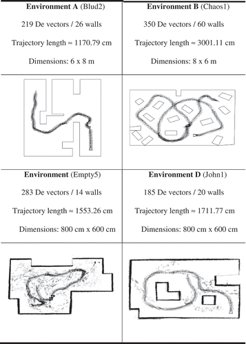
The sensorial data are used to create the noisy measurements as

where is a realization of a random variable with uniform distribution, , is the noise level. The noise bandwidth takes the following values for the function in the experiments:

And for the Cox’s algorithm:

The 2DLS used is Sick-PLS-100 and has 361 beams in 180° and works in a horizontal plane only.

Algorithms DE and PSO are not limited by the searching grid, and the chromosome of all individuals is represented by real numbers. The SGA and aGA use a binary representation of the chromosomes with 32-bit length; 16-bit for every coordinate. The mesh size of the grid used is 1 × 1 cm. The heading resolution is 0.5° for all 2D methods. The heading is computed separately by brute force. It is not included in evolutionary computations. The classification of the correct pose estimation uses quadratic averages from the list of values defining the best estimation of every pose (i.e. for every vector), separately for axis, axis, and heading . Standard deviations of values will be expressed as , , . Equations are:

(9)

and similarly for and . Reference poses “” were obtained by brute force using Equation (8) for zero noise level. The robot heading is considered with regard to the axis . Other monitored values are: function in ( strategy, one beam is considered a strip of width of 1 cm) and the standard deviation for values, classification function of the Cox algorithm is in and the standard deviations for it. Also the trajectory length in . All results are considered from the noise level of cm. For the selected levels of additive noise, the estimated trajectory is displayed—or all vectors—see Figures 4, 5, and 6. Working parameters of the EA: SGA a aGA: Chromosome is binary coded, 32-bit length, , , elitist selection, , two-point crossover, 5 randomly selected pairs from . The mutation is elitist, applied to two randomly chosen individuals in the population. The mutation changes all bits of the chromosome: the new position of every individual will be situated randomly to a small oblong of cm around the best individual in the population. The replacement strategy replaces the eight worst individuals in the population. The aGA (Moravec 2012) has identical working parameters as the SGA, but the aGA uses two 32-bit length chromosomes. operator parameters: , elitist mutation , see Leung and Liang (2003). DE algorithm: perturbation vector is rand/1/exp, , , , . PSO: , , . The searching area is identical for all EA as: 60 × 60cm. Cox’s algorithm: detection angle with step 0.5°, grid spacing was 1x1cm, searching area cm, convergence termination condition of the Cox algorithm is expressed as and is elected equal to . 2DLS used is Sick-PLS-100 – see (Sick 2000).

EXPERIMENTAL RESULTS

In order to test the (L1-norm) and Cox (L2-norm) algorithms, four real environments built of article boxes were considered; see Figure 1. Such type of environments can be found in manufacturing halls, offices, stocks, etc. Dimensions are approximately 6 × 8 meters. This corresponds to the abilities of 2DLS that was used and which has, based on the manufacturer’s recommendation, maximum usable measurable distance of 8–10 meters. However, only within the range of 0.6–5 meters is the accuracy with potential deviation of cm guaranteed, and moreover, ideal working conditions are required. The experiments in environments without moving objects form the main part of this article. The article also includes results of behavior of the tested algorithms in environments C and D with several moving objects—pedestrians that will serve for a comparison of characteristics of the 2D and 3D optimizers (Kwok et al. 2006) and 2D L2-norm Cox gradient algorithm.

Computational Costs

The required time is measured for a scenario when all 361 beams are actively used in the computation, which is reflected by the time demands; see Table 1. All calculations were performed using the 1×CPU: AMD AMD3500+/Orleans/2.2GHz. As the tested environments were built with different numbers of lines, only the time requirements for identical environments can be compared.

TABLE 1 Time Demands in [min], Zero Noise Level

Algorithm	Environment A	Environment B
+ SGA	14.68*/33.66/1.28^#	47.23/3.22^#
+ aGA	14.23*/32.15/1.26^#	54.23/3.22^#
+ PSO	30.14/1.33^#	59.13/3.47^#
+ DE	33.83/1.36^#	68.76/3.49^#
COX – HC	103.21	589.18
COX – BF	432.12	870.32

For all EAs tested, the time demands are almost identical. This is caused particularly by the small number of individuals and generations. In cases when only a half of this number of individuals is used, the time demands are proportionally lower by one half as well (see the algorithms SGA and aGA—Table 1). The average time for + EA which is necessary for the estimation of the trajectory with length of 1156.4 cm in environment A is 32.44 minutes. The DE has the highest time demands of all EAs used, approximately 1 minute above the average. In the case of the trajectory in environment B, the measured time is 68.76 minutes. The Cox gradient algorithm is significantly more time demanding. In the environment A, time demands were 103.21 minutes, in the environment B, 589.18 minutes. The acceleration of calculation enables the use of a larger grid mesh and a smaller number of 2DLS beams, but at the cost of lower accuracy. Table 1, serving only as a comparison, contains time demands for the Cox algorithm using brute force. In the environment A, the time was 432.12 minutes and in environment B, 870.32 minutes. With regard to the improvements that were proposed by Lu and Milios (1997), using the brute-force approach is not justified.

Time for the whole trajectories in tested environments; , , , (*) = Number of individuals in population is 10. BF = brute force algorithm. HC = HillClimbing (classic gradient) algorithm in an 8-connected neighborhood. Cox-HC, Cox-BF: detection angle is . (^#) = Smaller, yet well usable number of , is used for all tested algorithms: , , .

Inaccuracy at Pose and Heading Estimation

Sensorial data obtained from the robot passing the environments were for subsequent processing burdened by an additive noise; Uniform distribution. The simulation was launched and all the tested and Cox algorithms had to find the correct trajectory, supposing that only the sensorial data from 2DLS were available, i.e., no odometry. The start pose in the environment A is , in the environment B it is . For both tested algorithms , Cox identical trajectories are used. The environment A is an s-shaped corridor, the environment B is a large room with many static objects, distributed randomly across the whole area.

In both cases, the robot passed along a random trajectory. The number of vectors in the environment A is 219, in the environment B it is 350. Once the sensorial data were obtained from 2DLS, they were inserted into the navigation algorithm to estimate the correct poses and trajectory. Graphs (see Figures 2–11) display the inaccuracy of the pose and heading estimation from the noise level of cm. All vectors are displayed, too. The sensorial data were gradually burdened by the additive Uniform noise with a zero mean and the whole experiment was repeated until the estimator failed. Resulting values are depicted separately for axes and angle – heading regarding the axis . Each point in the graph represents the average of the whole trajectory at the selected level of additive noise. The L1-norm estimator based on the method provided a very stable and robust tool for pose estimation purposes. It is evident in Figures 2, 3, 4, and 5 that for example in the environment A, no malfunction occurred, neither at the highest noise levels with noise bandwidth of 800 cm (). The robot managed to reach the target point. In the environment B, the result of the situation was very similar. The estimator systematically failed when the highest levels of noise with noise bandwidth higher than 600 cm () was reached. Basically, none of the estimators was able to work properly at such level of noise stress and it randomly failed. There is only one exception: the algorithms SGA and aGA were able to navigate the robot successfully to the requested target in 1/10 cases to 1/15 cases, but only if the test was repeated.

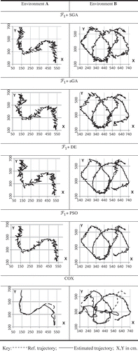
FIGURE 2 SGA algorithm; the estimated trajectory, noise bandwidth in [cm]; the sensorial data are plotted over a geometrical map.

FIGURE 3 aGA algorithm; the estimated trajectory, noise bandwidth in [cm]; the sensorial data are plotted over a geometrical map.

FIGURE 4 DE algorithm; the estimated trajectory, noise bandwidth in [cm]; the sensorial data are plotted over a geometrical map.

FIGURE 5 PSO algorithm; the estimated trajectory, noise bandwidth in [cm]; the sensorial data are plotted over a geometrical map.

FIGURE 6 COX algorithm; the estimated trajectory, noise bandwidth in [cm]; the sensorial data are plotted over the geometrical map.

A test with the uniform crossover (Begum et al. 2006a) was conducted for both the SGA and aGA. Surprisingly, it showed that under such conditions, both algorithms provided slightly better results in comparison with the classic two-point crossover. The result of navigation for the Cox L2-norm algorithm is displayed in Figure 6. This algorithm has very limited abilities of robot navigation in an environment that is loaded by noise with the given characteristics. In no test was the noise level of 150 cm () exceeded successfully. Tests were conducted in other types of environments, for example, in a long corridor, an empty oblong-shaped room, but the results were always identical. In the following sections, all monitored values will be discussed in detail with regard to the 2D approach of the EAs estimators and the Cox gradient algorithm.

In the environments A and B and at the lower noise levels with noise bandwidth of 20 cm, all algorithms provided very stable and accurate results. The deviation from the ideal pose did not exceed 5 cm for and axes, and the deviation of the heading estimation was maintained under the value of 0.8°. With respect to the accuracy of the 2DLS used, it is possible to affirm that under such working conditions, it does not matter which type of algorithm is used because all algorithms provide almost identical and acceptable results. The accuracy of the 2DLS used is, under ideal conditions, 5 cm and because of incorrect reflections, the deviation can reach up to cm or more, depending on the measured distance. Differences between individual EAs in the environment A (see Figure 9) are the following: the best results are provided by the DE algorithm. The accuracy of the pose estimation with the added noise of 20 cm is 1 cm for axis and 0.5° for the robot heading. The PSO algorithm provides almost identical results.

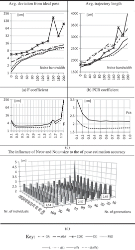
FIGURE 7 The values of the Fitness function and Cox’s objective function. Vertical axis in scale. White oblongs/cones/pyramids stand for algorithm malfunction. d(…) – standard deviation.

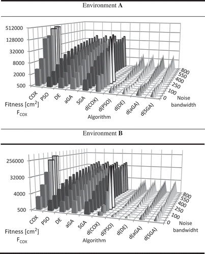
FIGURE 8 Trajectory length, algorithms: SGA, aGA, DE, PSO, and COX for increasing levels of noise, ▪ - algorithm failed.

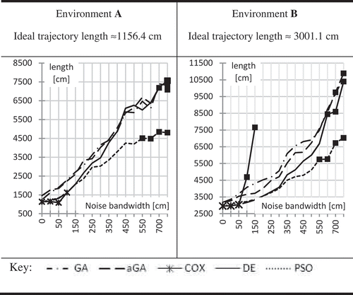
FIGURE 9 Environment A – The accuracy of pose and heading for increasing levels of noise, algorithms SGA, aGA, DE, PSO, and COX, Vertical axis in .

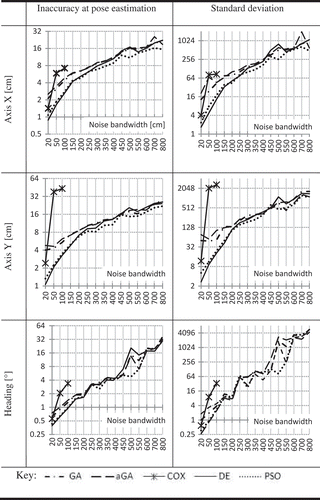
In comparison to DE, the PSO is worse; however, approximately by only 3%–4% and only at the lower noise levels with the noise bandwidth limit up to 50 cm. Then both methods are for a certain time almost identical in terms of efficiency. The disadvantage of PSO is the fact that it works with a double number of particles. However, the PSO is simpler with respect to the algorithmization. The same as any other EAs used, the PSO optimizes the function that is 2D, nonlinear, nonseparable, continuous, and unimodal; in a small area around the correct pose and under low noise levels—otherwise the function is strongly multimodal—see Lu and Milios (1997) and Censi (2008) and also Moravec and Pošík (2014). The use of all selected EAs including the PSO is justifiable. The disadvantage of the EAs used as an optimization tool is their tendency to a random malfunction, or, in other words, their premature convergence. This event was observed in 0.5% cases but only with the SGA and aGA algorithms and starting from the noise level of cm. Excluding the total and systematic malfunction of the algorithm at the noise with bandwidth of cm in the environment B, with the DE and PSO algorithms and at all lower levels of additive noise, this phenomenon was not observed in the environment A, not even in multiple repetitions of the test. In other words, in the environment A, for and for all tested EA, the navigation malfunction was observed beyond the limit defined by the highest noise load, in other words, at noise bandwidth wider than 800 cm. The measured accuracy of the pose and heading estimation for additive Uniform noise level of 20 cm : SGA: 2.12/4.01/0.62; aGA: 2.52/4.8/0.75; DE: 0.88/1.06/0.39; PSO: 1.08/1.33/0.43; Cox: 1.42/2.42/0.56. All EAs tested were able to navigate safely at the noise level of cm without any need to repeat the test, with the following results: SGA—21.21/27.32/36.35; aGA—18.86/24.27/31.89; DE—22.24/25.77/29.61; PSO—15.46/21.99/29.20. The Cox algorithm was able to navigate safely, even in repeating trials at the noise level with intensity of cm with the following results: 7.21/43.49/3.39. Figure 6 shows clearly that the navigation malfunction occurs when there is an imaginary trajectory compression to the detriment of the open area (area without objects). The value of the average deviation from the ideal pose corresponds to this behavior—in axis Y:43.49 cm in the environment A where the robot moves along the short corridor. This deviation is 7X bigger than the deviation in axis . It might seem that the structured environment B, where such places cannot be found, would show better results, but it is not so.

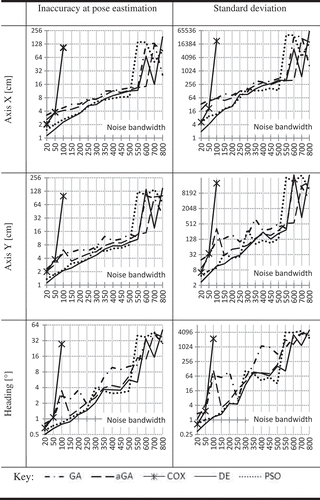
In the environment B (see Figure 10), the situation is almost the same as in A. Starting from the noise level of 100 cm, the PSO provides identical results as the DE. The SGA and aGA are worse in the pose and heading estimation, but still stable. The accuracy in axes and is 3 cm–4 cm with the heading of approximately 0.8° and with the noise level of 20 cm; and 6 cm/2° for the noise level of 150 cm. With higher noise levels, starting from the noise bandwidth of 250 cm, all methods used show almost identical results. The PSO is slightly better in comparison to DE, but the difference is insignificant. This phenomenon can be observed until the algorithm fails completely. In the environment B, the algorithm fails at the additive noise level of about 550 cm. Differences between SGA and aGA can be identified only with difficulties. The hybridization of the SGA or aGA algorithm does not provide significantly better results in terms of the continual robot localization task in comparison with SGA. Identical results were achieved in the structured or unstructured environment at lower and even at higher noise levels. The aGA has a small advantage: the navigation algorithm malfunction occurs at a noise level that is higher by 5%–7% in comparison to the SGA. Because of the two-chromosomal arrangement of every individual in the population, higher diversity is assured for the whole calculation time. In this case, the estimated trajectory is considerably chaotic, however, the robot managed to reach the target position. The trajectory becomes more chaotic with the extension of the noise bandwidth. Sometimes, the trajectory estimated by the algorithm becomes cyclic for several steps (vectors ), then the robot follows the correct trajectory again. The measured values of the inaccuracy of the pose and heading estimation for additive Uniform noise with bandwidth 20 cm are : SGA—3.27/ 2.32/ 0.81; aGA—2.60/ 2.06/ 0.71; DE—1.13/ 1.12/ 0.50; PSO—1.52/ 1.37/ 0.60; Cox—2.04/ 2.01/ 0.67. All EAs tested were able to navigate successfully at the noise level bandwidth of cm without the necessity to repeat the test(s), with following results: SGA—13.3/ 13.8/ 10.23; aGA—11.76/ 10.7/ 6.62; DE—11.37/ 9.18/ 5.631; PSO—8.48/ 8.02/ 4.43. The Cox algorithm was able to navigate safely even in repeated trials with the noise intensity of about cm with the following results: 7.21/ 43.49/ 3.39. Figure 6 clearly displays that the Cox algorithm at the noise level of was not able to navigate in the environment B and it failed approximately in 75% of the trajectory.

FIGURE 10 Environment B; The accuracy of pose and heading for increasing levels of noise, algorithms SGA, aGA, DE, PSO, and COX, Vertical axis in .

FIGURE 11 Referential and estimated trajectory at high noise level +/−225 cm.

The Cox gradient algorithm provides in the environment A and B stable results, but only up to the noise level of 20 cm, which is the lowest level tested. At the same time, it is necessary to state that up to this level, it is not possible to decide which of the tested methods provides better results, especially with regard to the type of the 2DLS used. The achieved accuracy of the pose estimation with the Cox algorithm with cm is only slightly worse than with the DE or PSO. For the axis it is 1.5 cm, for the axis it is 2 cm, and for the heading it is 0.5°. In comparison to , the results can be considered identical. With increasing additive noise level, the inaccuracy of the pose estimation for the Cox algorithm increases evenly for both axis and . The Cox algorithm permanently fails very early: at noise level of (exactly) 53 cm in the environment A and of 45 cm in the environment B. In practical usage, the Cox algorithm provides an ideal navigation tool for an environment without any disturbing influences.

Standard deviations of the monitored values and the angle have identical characteristics as the values, for both the and the Cox algorithms. Figures 9 and 10 show visible significant fluctuations, especially in the heading estimation in the structured environment B for the algorithms SGA and aGA. At the increasing levels of noise, the algorithm behaves in a way that the estimated pose has character of a random coordinate around the last found pose in the direction of the robot movement, or, along the ideal trajectory; however, the perpendicular distance from this point in the ideal trajectory never exceeds the value of approximately 50 cm–60 cm, not even at the noise level of about 700 cm–800 cm. With the Cox algorithm, smoothing of the trajectory arcs can be observed, for example, when the robot is turning around, when it turns in corridors, in offices, etc., and the curve verges to abscissa parallel with the corridor axis, or, with the axis of the free space. Chaotic pose estimations similar to the algorithm are not evident. The Cox algorithm fails unexpectedly. It is not possible to observe a gradual navigation malfunction similar to the . Sensorial data, vectors , are obtained from the 2DLS with frequency of 0.5 Hz. The robot moves inside the environment at the speed of about 5 cm–10 cm per second. To some extent, a local navigation malfunction of algorithm can be observed. Supposing that the robot speed is constant, this malfunction caused by an error in the pose and heading estimation can be corrected by increasing the number of vectors. This improvement does not work for the Cox algorithm. The sampling rate of the 2DLS used does not improve the Cox algorithm characteristics. In the unstructured environment A, the Cox algorithm’s malfunction occurred at the noise bandwidth of . Figure 6 displays clearly that the navigation fails after approximately 0.5 meters from the start pose. In the environment B, the situation is worse, the algorithm failed at the noise level bandwidth of about , in the half of the trajectory (i.e., after 15 meters).

Figure 7 displays characteristics of the function and the Cox classification function . Graphs of standard deviations of the values are displayed as well. Unlike with the Cox algorithm, where increases relatively steeply as well as the values, the values of the algorithm gradually decrease with the increasing noise levels, and, starting to form the noise level of 250 cm, gradually increase again. In comparison to the values, their characteristics are absolutely contrary. The values of the and Cox algorithms have gradually and linearly increasing characteristics. With the algorithm, the increase is more gradual in comparison to the Cox algorithm. Identical characteristics are evident in the environments A and B. The function indicates in both tested algorithms a difference between the real 2DLS scan area and the scan created by using the selected estimator, both in Cartesian coordinates.

In Figure 7, the bottom characteristics of the + SGA, aGA, PSO, DE functions are displayed. It is evident that all curves are linear. This phenomenon can be used to easily estimate the noise level in sensorial data. In the robotics area, a simple, effective, and easy algorithm to estimate a noise level in sensorial data does not exist. The advantage of the usage of the curves is that they are lacking some peaks. This effect simplifies all calculations. A great advantage is that such characteristics are identical in all environments, small, large, with some static objects inside the environment or without static objects, moreover, with or without moving objects. These characteristics are identical regardless of the additive noise level in the sensorial data.

Characteristics of the trajectory length are shown in Figure 8. The ideal trajectory length was obtained by measuring all distances between all points and individual vectors . In the environment A, the ideal trajectory length is 1156.4 cm, in the environment B it is 3001.1 cm. This experiment showed that the trajectory length remained almost identical at the increasing noise level, up to the noise level of about 50 cm () for the algorithms DE, PSO, and Cox.

In spite of the zero noise level, for the SGA and aGA algorithms, the trajectory length is longer by approximately 5%. The SGA and aGA provided, in both tested environments, almost the same trajectory length characteristics. In the structured environment B, the aGA is better. Starting from the noise level of approximately 150 cm for the unstructured environment A, and 250 cm for the structured environment B, the PSO shows the shortest trajectory length. For the noise level of 500 cm in the environment A, the trajectory length for the PSO is 4199.58 cm. This is the best obtained estimation. Nevertheless, this trajectory length is 3.6 times longer than in ideal working conditions. For all other algorithms, the trajectory length ranges between 6130 cm–6250 cm. In the environment B, the best estimated trajectory length is 5111.34 cm for the PSO algorithm, 6681.71 cm for the DE, and 6700 cm for the SGA and aGA.

Figure 11 displays in detail individual trajectories with the noise bandwidth of 450 cm (). The chaotic pose estimation described in the previous paragraph is evident in all tested algorithms + SGA, + aGA, + DE, and + PSO. If the figures were zoomed, it would became clear that in some places the trajectory is looped and it moves back against the correct robot direction movement for several vectors.

The situation is completely different for the Cox L2-norm algorithm. Starting from the zero noise level and until the algorithm malfunction occurs, the trajectory is completely smooth and continual, and singular estimated positions are connected smoothly. The disadvantage lies in the small resistance to an additive noise in sensorial data. In the case that a higher number of beams is overshadowed on one side of the 2DLS (for example, one half), the estimator tends to navigate the robot to empty areas, which are placed geographically on the opposite side of the 2DLS. With the Cox algorithm, no such thing was observed. If a certain number of beams is overshadowed, the Cox algorithm fails unexpectedly. In spite of the large number of experiments performed, a rule defining precisely how the static or moving obstacles have to be distributed to cause the unexpected failure of the Cox algorithm was not found, because the sensitivity at the edge of the Cox algorithm possibilities is high and more chaotic. The minimal number of beams equally distributed in the detection angle for the Cox algorithm that are needed in order to navigate successfully is approximately 25–30, and approximately 10–15 for the . The ability of both tested algorithms to work in the environment with moving objects and in the presence of noise will be briefly discussed in the following section.

3D Estimator and Environments with Moving Objects

In all the previous experiments, the continual localization algorithm using EA was handled in a way in which the used evolutionary estimator was working with the chromosome built of coordinates only. The heading estimation was performed by the brute force algorithm in a small angle (e.g., . The clear advantage of such an approach is the necessity of a smaller number of individuals in the population and a smaller number of generations for calculation. This approach ensures the higher calculation speed and good results. Naturally, it is possible to build the chromosome consisting of coordinates and heading angle . Such an approach can be found, for instance, in Kwok et al. (2006). However, experiments showed that to achieve good results in the continual robot localization task such as the general 3D optimization problem, the working parameters setting of the algorithms needed to be completely different. For example, a small number of individuals/generations always leads to the total navigation malfunction or, at least, to a significant estimator stability weakening. In this short experiment, the usage of the 3D algorithm will be examined. The DE was chosen because it provided stable results, though, not always the best results in all previous experiments.

The will be used for the continual robot localization in the environments C and D where there are several moving objects (2–3 pedestrians) while in the presence of an additive noise of various levels. The PSO would deserve our attention as well, however, it requires a double number of particles in comparison to the DE. Working parameters of the 3D DE estimator are: rand/1/bin, , , , (ideally see Figure 14), searching area 35 × 35 cm, , chromosome assemblage: , Uniform noise bandwidth in individual steps.

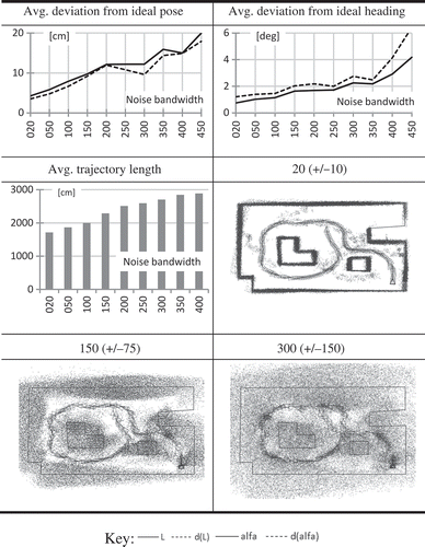
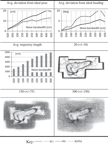
Figures 12 and 13 display the results of the experiment. The accuracy of the pose and heading estimation and standard deviations are the same as in the case of the 2D estimator. The additive noise resistance is identical as well. Figures 12 and 13 have the maximum noise bandwidth of 450 cm , but the estimator was able to operate even at the noise level of 600 cm–800 cm. Unlike in the environments A and B, where there were no moving objects, in the environments C and D random malfunctions of the 3D estimator can be observed, depending on the random distribution of moving objects, and maximum suitable noise stress seems to occur at the noise level of about 450 cm and seems to be from a practical point of view. Approximately 30% of all beams were always available for navigation. Values of the average trajectory length (noise bandwidth/trajectory length) in the environment C are 20 cm/1553.26 cm, 400 cm/4939.11 cm, and 20 cm/1711.77, 400 cm/2888.33 cm in the environment D. The trajectory length at a low noise level is almost identical to the ideal trajectory length. With regard to the 2D Cox algorithm possibilities, the 3D estimator is preferable and faster, and it provides stable results even at a higher noise levels (see Figures 2–13). Figure 14 shows a graph of average deviations from the ideal pose in the environment D for all tested algorithms 2D and the 2D Cox algorithm. It is clear that in the environment with moving objects, the Cox algorithm provides worse, but still stable, results—SGA:2.82; aGA:2.8; DE:1.11; PSO:2.89; Cox:5.7 cm. The accuracy of the heading estimation values has identical characteristics. The decrease of accuracy of the correct pose and heading estimation at an increasing noise level is gradual as in the case of the 3D estimator. In the environment D, the Cox algorithm was able to work even at the noise level of cm (see Figure14), and then it failed unexpectedly. The accuracy curve for the pose and heading estimation in the environments with moving objects for the Cox algorithm is moving slowly up along the axis, and proportionally to the number of overshadowed beams, or, to the number of moving objects. The minimum “rational” number of beams necessary to the navigation is approximately 25–30, supposing that all other parameters will be preserved, including the grid spacing :1 × 1 cm. With a lower number of beams, the Cox algorithm fails permanently. If the number of beams is lower than 90, in the environment D, random malfunctions depending on moving objects configuration can be observed. 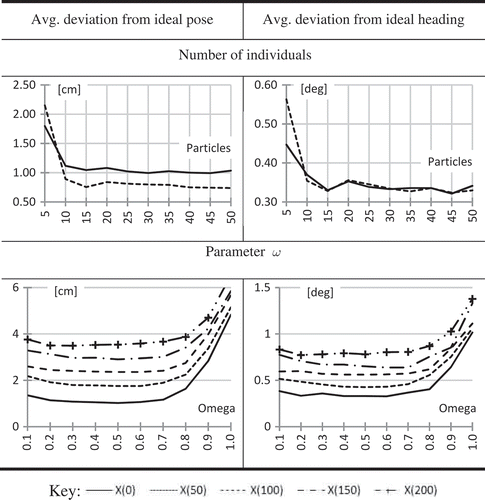Figure 14 also shows the dependency graph of the and values with reference to the accuracy of the pose and heading estimation and also the influence of the values. All values are meant for the tested perturbation vector rand/1/bin. Each of the 10 basic tested perturbation vectors (Storn 1996; Storn and Price 1997) provides slightly different results. The suitable range of the parameter values is and this range is applicable to all tested perturbation vectors.

FIGURE 12 Environment C (empty5) – Algorithm + DE 3D. Inaccuracy for pose and heading estimation + trajectory length + graphic representation of the estimated trajectory for increasing levels of noise. Point cloud is plotted over map and represents all sensorial data.

FIGURE 13 Environment D (john1) –Algorithm + DE 3D. Inaccuracy for pose and heading estimation + trajectory length + graphic representation of the estimated trajectory for increasing levels of noise. Point cloud is plotted over the map and represents all sensorial data.

FIGURE 14 Environment D, 2D, (a) Inaccuracy at pose estimation, (b) trajectory length. (c) Environment B, 3D. The influence of the F and PCR coefficient to the accuracy of pose estimation. (d) Environment B, 3D. The influence of variable N_POP and N_GEN to the accuracy of pose estimation.

L1-L2-norm Advantages and Disadvantages

The Cox algorithm is based on the point-to-line metric and it is possible to define it as a typical L2-norm algorithm. All experiments showed that this type of algorithm was only slightly resistant to the additive Uniform noise. It provides promising results at the lower noise levels, up to the level of about 10 cm. It plays no role if 4- or 8-connected neighborhoods are scanned. With an increasing noise level, the convergence speed to the correct solution decreases very slowly; see Figure 15. At the zero noise level, the time necessary for the robot to localize in an unstructured environment is 94.51 minutes, and 133.44 minutes with the maximum noise stress. Time demands increase slowly. Slightly more robust results can be achieved only if instead of the gradient optimizer (classic HillClimbing) searching, for instance, in an oblong/circular area by brute force is used, or if a suitable evolutionary estimator is used. The stability and accuracy of estimation provided by both options is higher only by 8%–10%, regardless of the type of environment. In the case of the continual localization, the Cox objective function is always continuous, unimodal, and nonseparable (supposing that the noise level is low, otherwise the function is multimodal). The start pose and the heading of the robot needs to be known for a successful localization. That can be determined, for instance, by using a global localization algorithm or it can be given a priori (by hand). The Cox algorithm can be used for global localization purposes as well. The algorithm has identical features. In case of global localization, time demands are significantly higher, however, they are proportional to the continual localization algorithm.

FIGURE 15 Cox’s algorithm time demands at increasing noise level.

The algorithm provides stable results even at the higher additive noise levels. In an unstructured environment such as corridors, hallways, and empty rooms, the algorithm is able to navigate successfully even at the noise level with bandwidth of about 600 cm–800 cm. This represents a situation in which the robot is passing through a place with small or large flying solid particles that poorly reflect the laser beams. When both tested methods work with identical 2DLS beams, the algorithm is faster and significantly more robust than the gradient Cox algorithm. The advantage of the algorithm is the fact that at an increasing noise level and because of usage of the evolutionary optimizers, the time of the pose estimation is still constant. With the Cox’s gradient algorithm, time demands are increasing, although very slowly. If the number of particles/generations of the EA is increasing, the results of the pose and heading estimation accuracy remain the same. Only the number of malfunctions with the SGA and aGA optimizers is decreasing, and the curves of the pose and heading estimation in graphs becomes smoother. Because of the accuracy of the 2DLS used, it is not possible to decide which of the tested methods, or Cox, is better at the zero noise level. Both algorithms provide accurate results. Using EA as a powerful optimizer of the 2D function is, in the surveyed case, very beneficial. If an identical problem is addressed in the same way as the 3D optimization task—see Kwok, Liu, and Dissanayake (2006)—time demands significantly increase. If the number of working parameters of the chromosome of individuals in the population chosen is too high (see Ebner 1999) time demands are very high as well. Such approach requires the individuals and generations to be at least by an order of magnitude larger to successfully converge. If the number of parameters of the chromosome is decreased adequately, see for example Moravec (2001), the task becomes less time demanding without compromising the robustness.

Summary

In their article, Moreno et al. (2002) presented the SGA algorithm as suitable for localization purposes in connection with the probability occupancy grid. Their algorithm reached the highest accuracy of the pose and heading estimation of about 3.5 cm in axes XY, and the largest deviation of heading was 1°. Data obtained in this experiment show that when the SGA is used in localization methods based on algebraic criteria, their results are equally good. The same was observed with the L2-norm Cox algorithm. Regarding the achieved results of all tested methods, it can be stated that the algorithms , provide stable results that are accurate enough, both at the zero noise level and at the higher noise levels. The is, however, to some extent limited and at the noise level of about 550 cm it is not able to operate correctly and effectively anymore. It fails particularly in a structured environment. The Cox gradient algorithm is absolutely unsuitable for a navigation under higher noise stress. On the contrary, at the zero noise levels, the differences cannot be measured. With reference to the achieved results, the best possible method of implementation is switching the various types of localization strategies; at the lower noise levels, (or or Cox) can be used, starting from the noise level of about 150 cm–200 cm up to 500 cm, the best results are provided by the algorithm, and starting from the noise level of 500 cm, the best possible results are provided by the or algorithm with a uniform crossover. In this approach, the algorithm is significantly more demanding, but it delivers the best possible results. In Begum et al. (2006a), the authors used the uniform crossover operator, tested in this study as well. Based on all performed experiments, it was found that the uniform crossover operator was able to provide higher stability for the algorithms, especially at the higher noise levels, but at the expense of about 10% higher malfunctions rate, especially at the highest noise levels starting from the noise bandwidth of 500 cm. If the navigation is failing, it is possible to repeat all calculations, which should lead to an improvement of the result. 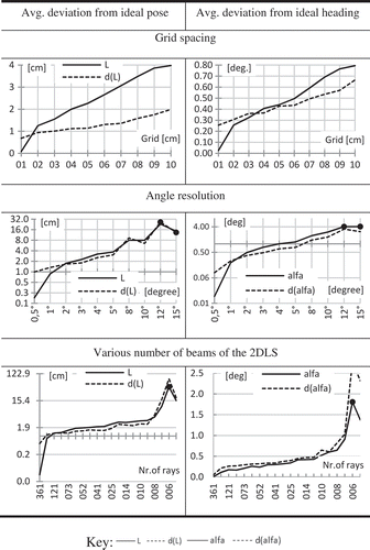If the grid mesh spacing in axes, detection angle, and number of beams are preserved, all working parameters of the 2D/3D evolutionary estimators for continual localization task can be constant. The time demanding run-time parametric adaptation of the working parameters is not necessary. With the Cox algorithm the same conclusions were drawn.

CONCLUSION

In this article, the comparative study dealing with the two most frequently used regularization schemas in the robotics area—robot navigation using 2DLS in an indoor environment, namely L1-norm and L2-norm—was presented. The algorithm representing typical L1-norm method is extended by several modern evolutionary optimizers: SGA, aGA, DE, PSO. All used EAs significantly accelerate the calculation of the robot pose and heading estimation and preserve the identical algorithmic stability in comparison to the original method. As the typical L2-norm representative, the algorithm called Cox was selected. In order to achieve the best possible results, the original gradient form of the Cox method is presented here. The Cox method is designed to operate in a purely polygonal common indoor office environment, similarly to the algorithm.

Hence, the mobile robots are successful in the real environments only if all proposed navigation methods are able to navigate successfully in the presence of various types of noise. In the current study, both algorithms, and Cox, were compared in working conditions of a common office environment under various levels of additive Uniform noise and in the environments with moving objects. The presented study described the advantages, disadvantages, accuracy, and abilities of all used evolutionary estimators. Based on all achieved results, it is evident that the results of both tested methods are identical, especially at the zero noise level, and it is possible to use these methods for navigation purposes in common office indoor environments.

Unfortunately, during the experiments, no method was found that would be capable of providing the best possible results under all circumstances—at high or low noise levels, in an environment with or without moving objects. From this point of view, the most suitable scheme is such in which a specific pose estimator for a specific environment and especially for specific noise level is used. For example, at zero or low noise levels the Cox algorithm, or (or, alternatively, ) provide great results. However, the optimizer requires a higher number of particles in the population. In tests that included pedestrians moving in selected environments, only cases with no complete overshadowing of the beams of the 2DLS and all resting beams approximately equally distributed in the detection angle of the used 2DLS were considered. The aGA algorithm provided average results. At the increasing level of noise and in the environments with moving objects, the SGA optimizer showed the worst results. The Cox algorithm is absolutely unusable in any environment with high noise level disturbances and it fails systematically. It is possible to use the Cox algorithm in an environment with several moving objects (1–2) if there is no significant overshadowing of the 2DLS beams. The aim of this study was to compare in practice all the selected methods, to compare the efficiency of typical representatives of the L1-norm and L2-norm algorithms, or, two metrics: point-to-point and point-to-line, commonly used for mobile robot navigation purposes in the mobile robotics area, and to decide under which conditions it is possible to use the individual estimators.

ACKNOWLEDGMENT

I would like to express my cordial thanks to the JanaČerná agency for text-linguistic corrections.

APPENDIX

In this section, various types of working parameters setting for all tested 2D algorithms will be described. Correct settings of all working parameters have a significant impact on the final results. An unsuitable setting usually leads to the total evolutionary estimator malfunction. The number of possible settings is very high for some tested EA, hence, only some combinations were selected.

• DE: The efficiency of the DE depends not only on the parameters. There are other important parameters such as , , , searching area dimensions, problem dimensionality, etc.

Price and Storn (1996), Price (1996), Price et al. (1999) based their definition of the set of possible settings on large practical experiments; for example , , where is a problem dimensionality. Ten basic perturbation vectors were examined: best/1/exp, rand/1/exp, randtobest/1/exp, best/2/exp, rand/2/bin, rand/2/exp, best/1/bin, rand/1/bin, randtobest/1/bin. rand/1/exp proved to be the best pert. vector for continual localization purposes found in the searching area of 100 × 100 cm. parameter values within the range of are suitable for all tested vectors regardless of the type of environment tested. The most suitable setting of the coefficient was found within the range of . The lowest values can significantly “afflict” the time demands.

• PSO: the algorithm has three working parameters . Based on their own experimental results, Kennedy and Eberhart (1995) built a large database containing recommended working parameters settings for most commonly addressed problems. Lower values lead to a decrease of the convergence rate, higher values lead to the PSO instability. Figure A5 displays results of tests of the parameter for various additive levels of the Uniform noise stress. The suitable values were found within the range of . This parameter does not depend on the type of environment, nor on the number of particles. The PSO usually requires a significantly higher number of particles. This aspect can be found as early as in Kennedy and Eberhart (1995), Barrera and Coello (2009). Figure A5 shows results of the pose accuracy estimation for a varying number of particles. Stable results can be reached if or higher, searching area 100 × 100 cm.

• and Cox algorithm – Figures A1 and A2 show the behavior of the and Cox algorithm, independent on type of the environment, if the “grid spacing (searching area)” is variable. [cm]: 1 × 1 (31 × 31), 2 × 2 (41 × 41), 3 × 3 (41 × 41), 4 × 4 (51 × 51), 5 × 5 (61 × 61), 6 × 6 (81 × 81), 7 × 7 (121 × 121), 8 × 8 (121 × 121), 9 × 9 (161 × 161), 10 × 10 (201 × 201). Cox: 1 × 1 (17 × 17), 2 × 2 (21 × 21), 3 × 3 (21 × 21), 4 × 4 (25 × 25), 5 × 5 (31 × 31), 6 × 6 (41 × 41), 7 × 7 (61 × 61), 8 × 8 (61 × 61), 9 × 9 (81 × 81), 10 × 10 (101 × 101). The brute-force algorithm was used in the tests. Both tested methods were able to operate properly if the grid was 10 × 10 cm, but the results were evidently worse. No malfunction was observed. The angle resolution was set to 0.5°. The behavior of all tested algorithms for various set of values is recorded in Figure 11. The scan angle resolution and detection angle: , , , , , , , , , . The largest and most practically usable angle resolution provided that the noise is set to the zero level: 10° for the algorithm and 4° for the Cox algorithm. If the lowest value is used, the algorithms become more robust and resistant to the additive noise and contrary. The number of 2DLS beams has a significant impact on the time demands. The number of beams in the test was selected as follows: 361, 181, 121, 91, 73, 61, 52, 46, 41, 33, 25, 18, 14, 12, 10, 9, 8, 7, 6, 5. The grid spacing was 1 × 1 cm, the angle resolution was 0.5°. Figures A1 and A2 show all results. The Cox method is able to operate with minimal number of beams of 18, with 7, but then the stability is lower. Both algorithms are at (rather over) the edge of stability. They were tested at the zero noise level.

  FIGURE A1 algorithm, the influence of the working parameters to the accuracy of pose and heading estimation, L- average deviation from the ideal position, d(L) – Std. dev., “alfa” – average deviation from the ideal heading, d(alfa) – Std. dev., • - algorithm failed.

  

  FIGURE A2 Cox algorithm, the influence of the working parameters to the accuracy of pose and heading estimation, L- average deviation from the ideal position, d(L) – Std. dev., “alfa” – average deviation from the ideal heading, d(alfa) – Std. dev., • - algorithm failed.

  

• SGA, aGA: The algorithms SGA and aGA have a relatively large number of working parameters. Unfortunately, a small change of any working parameter can lead to the total optimizer malfunction. The test of the behaviour of the algorithms was performed with various numbers of individuals/particles in population, i.e. : 4, 5, 6, 7, 8, 9, 10, 11, 12, 13, 14, 15, 16, 17, 18, 19, 20, 21, 22, 23. corresponds to the -population-SGA (). The searching area is small and the number of dimensions is low, hence, it was possible to use such setting. value corresponds to 50% of particles from . . The searching area was 100 × 100 cm, the detection angle , the number of beams 361. Figures A3 and A4 contains results of the test. Results are same for the SGA and aGA. The minimum number of individuals in population was found within the range of . The type of selection operator was tested too. Four different types of selection operators were chosen: (1) random selection method of number of individuals from , (2) roulette wheel, (3) elitistic selection that selects the k-th best individuals from the population and (4) tournament selection. All the other working parameters are identical as in the previous test. . The result of the test is displayed in Figures A3 and A4. The best possible results can be achieved if (3) and (4) selection operator is used. Random selection or tournament selection operators are unusable. Data displayed in graphs in Figure 12 represents the average of 10 trials. Four types of crossover operators were tested: one-point, two points, three-points and uniform crossover operator in various types of environments – structured and unstructured. One-point and three-points crossover operators showed very bad and unusable results. Two-points and uniform operators showed almost identical results, however, the results slightly differ depending on the type of environment in which the robot is moving and on the additive Uniform noise level. The mutation operator is usually used to preserve the population diversity. Three mutation operators were selected for the tests. The SGA and aGA variant without mutation operator was tested as well. Selected mutation operators are described in Table A1. Working parameters for SGA and aGA optimizers were identical as in the previous test. Results are recorded in Figures A3 and A4 and, again, represent the average of 10 trials.

  TABLE A1 Selected Types of Mutation Operators

  (1)	No mutation
  (2)	All bits of the chromosome will be randomly set to 0 or 1 value. An individual is selected randomly.
  (3)	One randomly selected bit of the kth number of the randomly selected individuals will be changed, i.e., original Holland’s mutation operator (Holland 1992). .
  (4)	Elitist mutation of the kth number of individuals. Chromosome obtains random value, which is selected as a random position from area size of around the best individual from . for all experiments.

  FIGURE A3 algorithm, the influence of the working parameters to the accuracy of pose and heading estimation, L- average deviation from the ideal position, d(L) – Std. dev., “alfa”– average deviation from the ideal heading, d(alfa) – Std. dev., • - algorithm failed.

  

  FIGURE A4 algorithm, the influence of the working parameters to the accuracy of pose and heading estimation, L- average deviation from the ideal position, d(L) – Std. dev., “alfa” – average deviation from the ideal heading, d(alfa) – Std. dev., • - algorithm failed.

  

  FIGURE A5 algorithm, the influence of the working parameters to the accuracy of pose and heading estimation. L- average deviation from the ideal position, d(L) – Std. dev., “alfa” – avg. dev. from the ideal heading, d(alfa) – Std. dev.; X(n)–noise bandwidth i.e., 0, 50, 100, 150, 200.

  

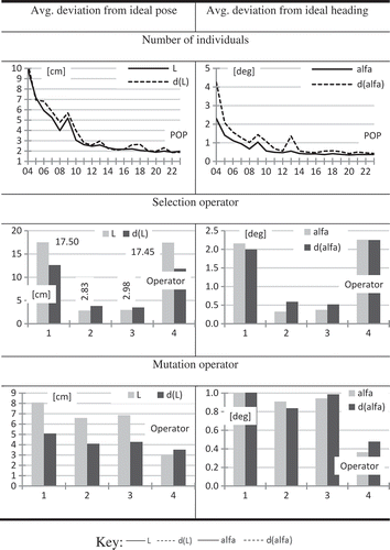
The elitist mutation operator showed the best possible results. Operators (2) and (3) provide identical results. The worst possible and almost unusable results are achieved if the mutation is omitted.

The presented experiments show only a small part of the potentially limiting values for algorithms and Cox. In the case that more working parameters are set at the edge of usability, it becomes clear that the systematic malfunction will appear more frequently and very soon. Such arrangement of working parameters was not tested. The advantage of the working parameters change at the running-time can be the significant calculation acceleration, for instance, if rational decrease in the number of beams of the 2DLS and larger grid mesh are used.

REFERENCES

- Barrera, J., and C.A.C. Coello. 2009. A review of particle swarm optimization methods used for multimodal optimization. Innovations in Swarm Intelligence. 248:9–37.
- Begum, M., G. K. I. Mann, and R. G. Gosine. 2006a. An evolutionary algorithm for simultaneous localization and mapping of mobile robots. In Proceedings of the IEEE/RSJ international conference on intelligent robots and systems, 4066–4071. IEEE Computer Society.
- Begum, M., G. K. I. Mann, and R. G. Gosine. 2006b. A fuzzy-evolutionary algorithm for simultaneous localization and mapping of mobile robots. In Evolutionary Computation, 1975–1982. Vancouver, BC: IEEE Congress on Evolutionary Computation.
- Begum, M., G. K. I. Mann, and R. G. Gosine. 2007. An Evolutionary SLAM Algorithm for Mobile Robots. Advanced Robotics, 21(9):1031–1050.
- Begum, M., G. K. I. Mann, and R. G. Gosine. 2008. Intergrated fuzzy logic and genetic algorithmic approach for simultaneous localization and mapping of mobile robots. Journal of Applied Soft Computing 8(1):150–165.
- Bektaş, S., and Y. Şişman. 2010. The comparison of L1 and L2-norm minimization methods. International Journal of the Physical Sciences 5(11):1721–1727.
- Besl, P., and N. McKay. 1992. A method for registration of 3-D shapes. IEEE Transactions on Pattern Analysis and Machine Intelligence 14(2):239–256.
- Bilgiç, B. 2010. Fast human detection with cascaded ensembles (Thesis, Massachusetts Institute of Technology, Cambridge, MA, USA).
- Borrmann, D., J. Elseberg, K. Lingemann, A. Nüchter, and J. Hertzberg. 2008. Globally consistent 3D mapping with scan matching. Journal of Robotics and Autonomous Systems 56(2):130–142.
- Burgard, W., D. Fox, D. Hennig, and T. Schmidt. 1996. Estimating the absolute position of a mobile robot using position probability grids. Paper presented at the Proceedings of the Thirteenth National Conference on Artificial Intelligence, 896–901, Portland, OR, August 4–8.
- Censi, A. 2008. An ICP variant using a point-to-line metric. In Proceedings of the IEEE international conference on robotics and automation ICRA 2008, 19–25. IEEE Press.
- Cox, I. J. 1991. Blanche – An experiment in guidance and navigation of an autonomous robot vehicle. IEEE Transactions on Robotics and Automation 7(2):193–204.
- Dellaert, F., D. Fox, W. Burgard, and S. Thrun. 1999. Monte Carlo localization for mobile robots. In Proceedings of the IEEE international conference on robotics and automation, 2:1322–1328. IEEE.
- Dielman, T. E. 1986. A comparison of forecasts from least absolute value and least squares regression. Journal of Forecasting 5:189–195.
- Diosi, A., and L. Kleeman. 2007. Fast laser scan matching using polar coordinates. The International Journal of Robotics Research 26(10):1125–1153.
- Ding, L. 2009. L1-norm and L2-norm neuroimaging methods in reconstructing extended cortical sources from EEG. In Proceedings of the International Conference of IEEE Engineering in Medicine and Biology Society 1( 2009):1922–1925.
- Dorigo, M.1992. Optimization, learning and natural algorithms (PhD thesis, Politecnico di Milano, Italy).
- Ebner, M. 1999. Evolving environment model for robot localization. Genetic Programming Proceedings of EuroGP99 1598:184–192. Berlin: Springer.
- Elfes, A. E. 1986. A sonar based mapping and navigation system. In Proceedings of the IEEE international conference on robotics and automation, 1151–1156. IEEE.
- Fox, D., W. Burgard, and S. Thrun. 1999. Markov localization for mobile robots in dynamic environments. Journal of Artificial Intelligence Research 11:391–427.
- Fu, H., M. K. Ng, M. Nikolova, and J. L. Barlow. 2006. Efficient minimization methods of mixed L2-L1 and L1-L1 norms for image restoration. SIAM Journal on Scientific Computing 27(6):1881–1902.
- Fuchs, H. 1984. Interactive bundle adjustment with metric and non-metric images including terrestrial observations and conditions. XVth ISPRS Congress A3:301–309. Rio de Janeiro: Committee of the XVth International Congress of Photogrammetry and Remote Sensing.
- Goldberg, D. E. 1987. Simple genetic algorithms and the minimal deceptive problem. In Genetic algorithms and simulated annealing, 74–88. London, UK: Pitman.
- Goldberg, D. E. 1989. Genetic algorithms in search, optimization, and machine learning. New York, NY: Addison-Wesley.
- Gomes-Mota, J., and M. I. Ribeiro. 1998. A multi-layer robot localisation solution using a laser scanner on reconstructed 3D models. Paper presented at Proceedings of the 6th International Symposium on Intelligent Robotic Systems, 213–222. Edinburgh, Scotland, UK.
- Gomes-Mota, J., and M. I. Ribeiro. 2000. Mobile robot localisation on reconstructed 3d models. Journal of Robotics and Autonomous Systems 31(1-2):17–30.
- Gorges-Schleuter, M. 1991. Explicit parallelism of genetic algorithms through population structures, 150–159. Berlin, Heidelberg: Springer-Verlag.
- Hahnel, D., W. Burgard, D. Fox, K. Fishkin, and M. Philipose. 2004. Mapping and localization with RFID technology. In Proceedings of the IEEE international conference on robotics and automation 1:1015–1020.IEEE.
- Holland, J. H. 1992. Adaptation in natural and artificial systems: An introductory analysis with application to biology, control, and artificial intelligence. Cambridge, MA, USA: MIT Press.
- Jin, Y., and J. Branke. 2005. Evolutionary optimization in uncertain environments-A survey. IEEE Transactions on Evolutionary Computation 9(3):303–317.
- Josselin, D., and D. Ladiray. 2001. Combining L1 and L2 norms for a more robust spatial analysis: The “Median Attitude.” Paper presented at the European Colloquium on Theoretical and Quantitative Geography. Saint-Valery en-Caux, France, September 7–11.
- Kennedy, J. and R. C. Eberhart. 1995. Particle swarm optimization. In Proceedings of the 1995 IEEE international conference on neural networks. Piscataway, NJ, USA: IEEE.
- Kummerle, R., G. Grisetti, H. Strasdat, K. Konolige, and W. Burgard. 2011. G2o: A general framework for graph optimization. In Proceedings of the IEEE International Conference on Robotics and Automation (ICRA), 3607–3613. IEEE.
- Koza, J. 1996. Genetic programming: On the programming of the computers by means of natural selection, 5th ed. Cambridge, MA, London, UK: MIT Press.
- Květoň, K. 1987. Method of averages as an alternative to L1- and L2-norm methods in special linear regression problems. Computational Statistics and Data Analysis 6(4):407–414.
- Kwok, N. M., D. K. Liu, and G. Dissanayake. 2006. Evolutionary computing based mobile robot localization. Engineering Applications of Artificial Intelligence 19:857–868.
- Lazanas, A., and J. C. Latombe. 1992. Landmark-based robot navigation (Technical Report, STANCS-92-1428, Dept. of Computer Science, Stanford University, Stanford, CA, USA).
- Leonard, J. J., and H. F. Durrant-Whyte. 1991. Mobile robot localization by tracking geometric beacons. IEEE Transactions on Robotics and Automation 7:376–382.
- Leung, K. S., and Y. Liang. 2003 Adaptive elitist-population based genetic algorithm for multimodal function optimization. Lecture Notes in Computer Science 2723:1160–1171.
- Lu, F., and E. Milios. 1997. Robot pose estimation in unknown environments by matching 2D range scans. Journal of Intelligent and Robotics Systems 18(3):249–275.
- Martin, M. C., and H. P. Moravec.1996. Robot evidence grid (Technical Report CMU-RI-TR-96-06, The Robotics Institute Carnegie Mellon University, Pittsburgh, PA, USA).
- Martin, F., L. M. Munoz, S. Garrido, D. Blanco, and L. Moreno. 2009. L1-norm global localization based on a differential evolution filter. Paper presented at the Proceedings of the IEEE International Symposium on Intelligent Signal Processing, 229–234. Budapest, Hungary, August.
- Maybeck, P. S. 1979. Stochastic models, estimation and control. NewYork, NY: Academic.
- Metropolis, N., and S. Ulam. 1949. The Monte Carlo method. Journal of the American Statistical Association 44:335–341.
- Mitchell, H. B. 2007. Multi-sensor data fusion: An introduction. Berlin, Heidelberg: Springer Verlag.
- Moravec, J. 2001. Continuous robot localisation in known environment using genetic algorithm. In Proceedings of the 10th IEEE international conference on fuzzy systems, 6. Melbourne, Australia: IEEE.
- Moravec J. 2012. Cascaded evolutionary estimator for robot localization. International Journal of Applied Evolutionary Computation (IJAEC) 3(3):33–61.
- Moravec, H. P., and Elfes, A. 1985. High resolution maps from wide angle sonar. In Proceedings of the IEEE international conference on robotics and automation, 116–121. IEEE Computer Society.
- Moravec J., and P. Pošík. 2014. A comparative study: The effect of the perturbation vector type in the differential evolution algorithm on the accuracy of robot pose and heading estimation. Evolutionary Intelligence Journal 6(3):171–191.
- Moreno, L., J. M. Armingol, S. Garrido, A. Escalera, and M. A. Salichs. 2002. A genetic algorithm for mobile robot localization using ultrasonic sensors. Journal of Intelligent and Robotic Systems 3(2):135–154.
- Moreno, L., S. Garrido, D. Blanco, and M. L. Muñoz. 2009. Differential evolution solution to the SLAM problem. Journal of Robotics and Autonomous Systems 57(4):441–450.
- Moreno L., D. Blanco, M. L. Munoz, and S. Garrido. 2011. L1–L2-norm comparison in global localization of mobile robots. Robotics and Autonomous Systems 59:597–610.
- Mozos, M. O., R. Triebel, P. Jensfelt, A. Rottmann, and W. Burgard. 2007. Supervised semantic labeling of places using information extracted from sensor data. Robotics and Autonomous Systems 55:391–402.
- Narula, S. C., P. H. N. Saldiva, C. D. S. Andre, S. N. Elian, A. F. Ferreira, and V. Capelozzi. 1999. The minimum sum of absolute errors regression: A robust alternative to the least squares regression. Statistics in Medicine 18(11):1401–1417.
- Narula, S. C., and J. F. Wellington. 1982. The minimum sum of absolute errors regression: A state of the art survey. International Statistical Review 50(3):317–326.
- Negenborn, R. 2003. Robot localization and Kalman filters (PhD Thesis, Utrecht University, The Netherlands).
- Nieto, J., T. Bailey, and E. Nebot. 2006. Scan-SLAM: Combining EKF-SLAM and scan correlation field and service robotics. Field and Service Robotics 25:167–178.
- O’Kane, J. M. 2006. Global localization using odometry. In Proceedings of the IEEE international conference on robotics and automation, 4084–4089. IEEE.
- Parsopoulos, K. E., V. A. Kontogianni, S. I. Pytharouli, P. A. Psimoulis, S. C. Stiros, and M. N. Vrahatis. 2004. Optimal fitting of curves in monitoring data using the L1, L1 and L∞ norms. Paper presented at the INGEO 2004 and FIG Regional Central and Eastern European Conference on Engineering Surveying, 1–9. Bratislava, Slovakia, November 11–13.
- Price, K. 1996. Differential evolution: A fast and simple numerical optimizer, In Proceedings of the biennial conference of North American fuzzy information processing society NAFIPS’96, 524–527. Piscataway, NJ, USA: IEEE.
- Price, K., D. Corne, M. Dorigo, and F. Glover, Eds. 1999. An introduction to differential evolution, 79–108. London, UK: McGraw-Hill.
- Price, K., and R. Storn. 1996. Minimizing the real functions of the ICEC’96 contest by differential evolution. Paper presented at the Proceedings of the IEEE International Conference on Evolutionary Computation, 842–844. Nagoya, Japan, May 20–22.
- Pronobis, A. 2011. Semantic mapping with mobile robots (PhD thesis, KTH Royal Institute of Technology, Stockholm, Sweden).
- Remolina E., and B. Kuipers. 2004. Towards a general theory of topological maps. Journal Artificial Intelligence 152:47–104.
- Sasaki Y., S. Kagami, S. Thompson, and H. Mizoguchi. 2007. Sound localization and separation for mobile robot tele-operation by tri-concentric microphone array. Journal of Robotics and Mechatronics 19(3):281–289.
- Sick, A. G. 2000. PLS proximity laser scanner. Installation and operation manual SICK-PLS-100. Germany: Author.
- Skrzypczynski, P. 2009. Simultaneous localization and mapping: A feature-based probabilistic approach, International Journal of Applied Mathematics and Computer Sciences 19(4):575–588.
- Storn, R. 1996. On the usage of differential evolution for function optimization. In Proceedings the biennial conference of the North American fuzzy information processing society NAFIPS’96, 519–523. Piscataway, NJ, USA: IEEE.
- Storn, R., and K. Price. 1997. Differential evolution—A simple and efficient heuristic for global optimization over continuous spaces. Journal of Global Optimization 11:341–359.
- Tanese, R. 1989. Distributed genetic algorithms. In Proceedings of the third international conference on genetic algorithms, 434–439. San Francisco, CA: Morgan Kaufmann.
- Thrun, S. 2001. An online mapping algorithm for teams of mobile robots. The International Journal of Robotics Research 20(5):335–363.
- Thrun, S., W. Burgard, and D. Fox. 2005. Probabilistic robotics. Cambridge, MA, USA: MIT Press.
- Yan, F., K. Mikolajczyk, J. Kittler, and M. Tahir. 2009. A comparison of L1-Norm and L2-norm multiple kernel svms in image and video classification. In Proceedings of the 2009 seventh international workshop on content-based multimedia indexing, 7–12. Chania, Greece: IEEE.
- Weiss, G., C. Wetzler, and E. von Puttkamer. 1994. Keeping track of position and orientation of moving indoor systems by correlation of range-finder scans. Paper presented at the Proceedings of the International Conference on Intelligent Robots and Systems, 1: 595–601. Munich, September 12–16.
- Weiss, G., and E. Puttkamer. 1995. A map based on laser-scans without geometric interpretation. Intelligent Autonomous Systems, 403–407. IOS Press.
- Whitley, D. 1994. A genetic algorithm tutorial. Statistics and Computing 4:63–85.
- Whitley, D., S. Rana, and R. B. Heckendorn.1998. The island model genetic algorithm: On separability, population size and convergence. Journal of Computing and Information Technology 7:33–47.
- Wilson, H. G. 1978. Least squares versus minimum absolute deviations estimation in linear models. Decision Sciences 9(2):322–335.
- Zhu,Q., S. Avidan, M. Ch. Yeh, and K. T. Cheng. 2006. Fast human detection using a cascade of histograms of oriented gradients. In Proceedings of the IEEE conference on computer vision and pattern recognition, 2:1491–1498. IEEE.