An Overview of Audio Event Detection Methods from Feature Extraction to Classification

ABSTRACT

Audio streams, such as news broadcasting, meeting rooms, and special video comprise sound from an extensive variety of sources. The detection of audio events including speech, coughing, gunshots, etc. leads to intelligent audio event detection (AED). With substantial attention geared to AED for various types of applications, such as security, speech recognition, speaker recognition, home care, and health monitoring, scientists are now more motivated to perform extensive research on AED. The deployment of AED is actually a more complicated task when going beyond exclusively highlighting audio events in terms of feature extraction and classification in order to select the best features with high detection accuracy. To date, a wide range of different detection systems based on intelligent techniques have been utilized to create machine learning-based audio event detection schemes. Nevertheless, the preview study does not encompass any state-of-the-art reviews of the proficiency and significances of such methods for resolving audio event detection matters. The major contribution of this work entails reviewing and categorizing existing AED schemes into preprocessing, feature extraction, and classification methods. The importance of the algorithms and methodologies and their proficiency and restriction are additionally analyzed in this study. This research is expanded by critically comparing audio detection methods and algorithms according to accuracy and false alarms using different types of datasets.

Introduction

Audio event detection (AED) is aimed at detecting different types of audio signals such as speech and non-speech within a long and unstructured audio stream. AED can be considered a new research area with the ambitious goal of replacing intelligent surveillance systems (ISS) with traditional surveillance systems (Kalteh, Hjorth, and Berndtsson 2008). Traditional systems require the regions of interest (ROI) that are equipped with cameras, microphones, or other sensor types to be constantly monitored by human operators who record audio data to multimedia datasets. A multimedia dataset often consists of millions of audio clips, for instance environmental, speech, and music with other non-speech noises to use in AED. The bases for most AED-related research fields and applications are feature extraction and audio classification. These are apparently significant tasks in many approaches employed in numerous areas and environments. They comprise the detection of abnormal events (gunshots) in security (Clavel, Ehrette, and Richard 2005), speech recognition (Choi and Chang 2012; Navarathna et al. 2013; Scheme, Hudgins, and Parker 2007), speaker recognition (Ganapathy, Rajan, and Hermansky 2011; Zhu and Yang 2012), animal vocalization (Bardeli et al. 2010; Cheng, Sun, and Ji 2010; Huang et al. 2009; Milone et al. 2012), home care applications (Weimin et al. 2010), medical diagnostic problems (Drugman 2014), bioacoustics monitoring (Bardeli et al. 2010; Cheng, Sun, and Ji 2010), sport events (Li et al. 2010; Potamitis et al. 2014; Su et al. 2013), fault and failure detection in complex industrial systems (Xu, Zhang, and Liang 2013), and several other fields. AED system performance, such as complications, classification accuracy, and false alarms, is extremely reliant on the extraction of audio features and classifiers (Dhanalakshmi, Palanivel et al. 2011b, Zubair, Yan et al. 2013).

Feature extraction is one of the most significant factors in audio signal processing (Dhanalakshmi, Palanivel et al. 2011a). Audio signals have many features, not all of which are essential for audio processing. All classification systems employ a set of features extracted from the input audio signal, where each feature represents a vector element in the feature space. Therefore, a number of different audio classification methods based on system performance evaluation have been proposed. These approaches mostly differ from each other in terms of classifier selection or number of acoustic features involved. From the perspective of decomposition, the extracted features are classified into temporal, spectral, and prosodic features. Audio classification is another major stage in audio signal processing and pattern recognition, with possible applications in audio detection, documentation, and event analysis. Audio classification refers to the ability to precisely classify the selected feature vectors in corresponding classes. Different classifier types, including manual classification, which is time consuming, supervised, unsupervised, and semi-supervised learning algorithms are employed to reduce classification problems.

A number of concerns relating to feature extraction and classification methods have been reviewed in existing literature. Lu (2001) reviewed a survey covering time and frequency domain features. Regarding speaker recognition, Kinnunen and Li (2010) reviewed features and speaker modeling and in another review Kinnunen et al. (2011) covered types of features and the best-known clustering algorithms in terms of accuracy. Prakash and Nithya (2014) reviewed a survey and addressed all aspects of semi-supervised learning algorithms. Bhavsar and Ganatra (2012) considered and compared machine learning classification algorithms in terms of speed, accuracy, scalability, and other traits. This has consequently helped other researchers study existing algorithms and develop innovative algorithms for previously unavailable applications or requirements.

Although hundreds of audio event detection methods have been proposed in various fields, unfortunately only a few extensive studies are actually devoted to surveying or comparing them. While most works on AED focus on some key acoustic events, none cover the state-of-the-art in AED. The present work differs from all previous efforts in terms of emphasis, timeliness, and comprehensiveness. The need for detailed and comprehensive studies on the vital aspects of AED methods has led researchers to orchestrate reviews of AED classification methods and algorithms. The goal of this review is to highlight the classification concerns and challenges with AED methods as a way to analyze audio event detection methods and algorithms from a range of perspectives. Furthermore, a comparative study is hereby presented based on key attributes, such as accuracy, false alarm, precision, and recall. These are considered the most recent advancements in this area for identifying future research trends that can greatly benefit both general and expert readers.

This review is structured as follows. Section 2 contains the research methodology. An overview of preprocessing, a feature extraction, and classification method is provided in Section 3. Section 4 consists of a discussion about the evaluation and performance of classification techniques with concerning to accuracy rate and an argument on the comparison of techniques and their accuracy based on reviewed articles. Finally, Section 5 presents some closing clarifications about this review.

Methodology

This review represents a detailed analysis of 66 different articles associated with audio event detection and classification in different systems. The criteria utilized to select sources of studies must contain a search mechanism that authorizes customized searches using keywords and titles. Access to downloading full articles is dependent on accessibility agreements between our university and the target digital library as the resource provider. The sources were obtained from different digital libraries including Science Direct, IEEE, and ACM with highly cited and credible publications, after which every study was checked to ensure the context is relevant to this review. This literature review includes problems that have hindered further developments in AED. Well-established researchers are interested in possible solutions related to the development of adequate AED, which is achievable through analyzing classification approaches and their performance. Table 1 presents literature works related to approaches that employ unsupervised, supervised, and semi-supervised learning algorithms. The list of journal-based articles expedites a general overview of the different classifiers pertaining to their characteristics. It also consists of the latest matters surrounding intelligent AED development in surveillance systems.

Table 1. Audio classifiers in AED.

Methods	Type of classifier	References
Unsupervised Learning Algorithms	Hierarchical and Partition Clustering	(Pomponi and Vinogradov 2013), (Tsunoo et al. 2011), (Park 2009), (Lefèvre and Vincent 2011) (Yang et al. 2013)
	Gaussian Mixture Models (GMM)	(Chuan 2013), (Choi and Chang 2012), (P. Dhanalakshmi et al. 2011b), (Cheng, Sun, and Ji 2010), (Chung-Hsien and Chia-Hsin 2006)
	Hidden Markov Models (HMM)	(Navarathna et al. 2013), (Niessen, Van Kasteren, and Merentitis 2013), (Itoh, Takiguchi, and Ariki 2013), (Wang and Zhang 2012), (Milone et al. 2012), (Ya-Ti et al. 2009), (Scheme, Hudgins, and Parker 2007)
	Neural networks(Self-organizing map, ART)	(P. Dhanalakshmi et al. 2011a), (Schroeder et al. 2011), (Charalampidis, Georgiopoulos, and Kasparis 2000)
Supervised Learning Algorithms	Instance-based or K-nearest-neighbors (KNN)	(Khunarsal, Lursinsap, and Raicharoen 2013), (Ravan and Beheshti 2011), (Liu and Zhang 2012), (Lie, Hong-Jiang, and Hao 2002), (Huang et al. 2009), (Malhotra, Nikolaidis, and Harms 2008)
	Neural Networks (RBF, MLP)	(Balochian, Seidabad, and Rad 2013), (Ganapathy, Rajan, and Hermansky 2011), (Mitra and Wang 2008), (Kotti et al. 2007), (Shen, Shepherd, and Ngu 2006), (Turnbull and Elkan 2005), (Khairnar, Merchant, and Desai 2005), (McConaghy et al. 2003)
	Rule-based Classifiers	(Xu, Zhang, and Liang 2013), (Alcala-Fdez, Alcala, and Herrera 2011), (Ruiz Reyes et al. 2010), (Temko, Macho, and Nadeu 2008)
	Ensemble Classifier	(Younghyun, Hanseok, and Han 2013), (Dafna, Tarasiuk, and Zigel. 2013), (Li, Wang, and Sung 2008), (Bin, Haizhou, and Rong 2007), (Meyer and Schramm 2006)
	Bayesian Networks	(Giannakopoulos, Pikrakis, and Theodoridis 2007), (Prodanov and Drygajlo 2005), (Daoudi, Fohr, and Antoine 2003), (Zweig 2003)
	Linear Discriminants	(Gergen, Nagathil, and Martin 2014), (Lu and Wang 2012), (Lee et al. 2006)
	Support Vector Machines	(Andreassen, Surlykke, and Hallam 2014), (Muhammad and Melhem 2014), (Costa et al. 2012), (Shuiping, Zhenming, and Shiqiang 2011), (Temko and Nadeu 2009), (Dhanalakshmi, Palanivel, and Ramalingam 2009), (Truong, Lin, and Chen 2007), (Temko and Nadeu 2006), (Acır, Özdamar et al. 2006)
Semi-Supervised Learning Algorithms	Self-training	(Triguero et al. 2014), (Neiberg, Salvi, and Gustafson 2013), (Santos and Canuto 2014), (Yanan et al. 2012)
	Co-training & EM	(Yunyun, Songcan, and Zhi-Hua 2012), (Cui, Jing, and Jen-Tzung 2012), (Yangqiu and Changshui 2008), (Moreno and Agarwal 2003)
	TSVM	(Guz et al. 2010),(Rongyan et al. 2010)

These studies analyze two crucial factors concerning the comparison of different AED methods’ performance. The first factor is the accuracy of classification steps and the second regards the false positives and negatives rate. Here, the importance of the proficiency and accuracy aspects will be emphasized. For example, Giannakopoulos, Pikrakis, and Theodoridis (2007) presented a multi-class audio classification method for recorded audio sections from movies. The method focuses on high-accuracy recognition of violent content in order to protect sensitive groups (e.g. children). Schroeder et al. (2011) managed to achieve a low false positive rate of less than 4% except for the knocking event. Muhammad and Melhem (2014) attained the high accuracy of 99.9% (with a standard deviation of 0.15%) in the detection of pathological voices. They also achieved up to 100% accuracy for binary pathology classification. Each of these algorithm techniques is normally applied on a sample dataset for training and testing. For example, Table 2 displays six major benchmark datasets: GTZAN, RWCP-DB, AVICAR, LVCSR, Aurora-2, and Ballroom. The proposed methods’ generalization performance is analyzed and evaluated. Due to the extremely hazardous nature of operating AED systems in real-life environments, it is very difficult and complicated to perform real-time testing. Generally, many researchers prove their observations by creating experimental simulations that artificially depict real environments to analyze recognition rate performance.

Table 2. Types of datasets for AED.

Dataset Name	Dataset Type	Description
AVICAR (Navarathna et al. 2013)	Speech and Event	AVICAR is a speech dataset recorded using multi-sensory arrays containing four video cameras and eight microphones in a car environment. Speakers of various languages include 50 males and 50 females.
GTZAN (Tsunoo et al. 2011)	Music/Speech	GTZAN is a dataset containing 20 musical genre and 3 speech excerpts with different qualities, each excerpt being 30 seconds long.
Aurora-2 (Truong, Lin, and Chen 2007)	Speech	Aurora-2 is a dataset of recorded hands-free speech to explore the influence on automatic speech recognition performance in noisy situations.
RWCP-DB (Temko and Nadeu 2006)	Event and Environment	RWCP-DB is a dataset with 105 environmental sound events and around 100 anechoic samples of each event in 3 categories: first, collisions such as wood; second, actions like articles dropping; third, characteristics such as small metal articles, paper and instruments.
LVCSR (Meyer and Schramm 2006)	Word Dataset	LVCSR is a rich word dataset when the testing audio is a word stream. This dataset can produce very fast queries with high accuracy, and it is easy to add to, and enhance it to address current issues.
Ballroom (Shen, Shepherd, and Ngu 2006)	Music/Speech	Ballroom is a dataset containing excerpts of many music pieces with real radio quality (low quality)

Audio event detection systems

The audio event detection system presented in Figure 1 has three essential processing levels: preprocessing, feature extraction, and audio classification. The preprocessing step is responsible for increasing method robustness and for easing analysis by highlighting the appropriate audio signal characteristics.

Figure 1. Block diagram of an audio event detection system.

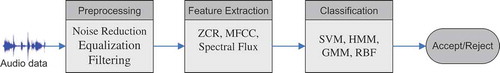
The feature extraction section initially converts a processed audio signal into attribute feature vectors based on suppressing redundant audio signals before extracting the features. Each feature represents an element of the feature vector in the feature space. A suitable model is developed in the final stage, followed by training to map the features to certain audio classes when important audio features are extracted. System efficiency relies on the capability to recognize and classify audio signals according to audio characteristics or content by using machine learning methods (Dhanalakshmi, Palanivel et al. 2011b). The emphasis of this overview is on classification methods. The subsequent sections present a brief outline of preprocessing and feature extraction for the purpose of completeness.

Preprocessing

It is critical to perform pre-processing on input audio signals in order to develop a robust and appropriate audio signal representation. In general, an audio signal recorded with a microphone in the real world comes with a combination of background noise and foreground acoustic objects. This audio cannot be used straightaway as an input for machine learning-based classification. The reason is that signals contain redundancy, which first needs to be removed. The preprocessing step involves noise reduction, equalization, low-pass filtering, and segmenting the original audio signal into audio and silent events to be used in feature extraction.

Feature extraction

Feature extraction has a vital role in evaluating and characterizing audio content. Audio features are extracted from the audio signal frames. The ideal feature characteristics are: a) easy adaptability, b) robustness again noise, c) easy implementation, and d) contains the necessary smoothing characteristics (Uncini 2003). The number of feature space dimensions is equal to the number of extracted features. If the quantity of selected features is too high, a dimensionality problem occurs (Jain, Duin, and Jianchang 2000). Traditional techniques such as Gaussian mixture model are not able to handle high-dimensional data (Reynolds 1995; Reynolds, Quatieri, and Dunn 2000). Figure 2 classifies features into (1) temporal, (2) spectral, and (3) prosodic features. Temporal features directly designate the audio signal waveform for analysis. Low-level features are usually extracted via spectral analysis (frequency domain) of the audio signal. Prosodic features have a semantic meaning in the context of auditory perception. Consequently, as soon as a feature is extracted, any type of classifier can use the prosodic features to classify the samples into suitable groups.

Figure 2. Feature categorization.

1. Temporal Features

Temporal features, or time amplitude, are represented as amplitude fluctuation with time (waveform signal). Temporal audio features are extracted directly from raw audio signals with no preceding data. Representative instances of temporal features are zero-crossing rate, amplitude-based features, and power-based features. Such features normally suggest a simple tactic to investigate audio signals, although it is generally necessary to combine them with spectral features. Therefore, the computational complexity of temporal features is lower than that of spectral features.

1. Short-term energy

Short-term energy signifies audio signal loudness (Giannakopoulos and Pikrakis 2014; Lamel et al. 1981; Li et al. 2001; Lu 2001; Reaves 1991; Tong and Kuo 2001; Ye, Zuoying, and Dajin 2002). Short-term energy is computed according to the following equation (Giannakopoulos and Pikrakis 2014), where is the sequence of audio samples in the ith frame and is the frame length.

(1)

• (b) Zero-Crossing Rate (ZCR)

The Zero-Crossing Rate (ZCR) of an audio frame stands for the number of times the audio signal passes the zero signal in a unit of time or audio signal sign changes (Li et al. 2001; Lu 2001; Tong and Kuo 2001; Ye, Zuoying, and Dajin 2002). In other words, the number of times the value of the signal changes from positive to negative or vice versa is divided by the frame length. To a certain extent, ZCR connotes the specification of the signal spectrum, thus it approximates the signal spectral nature. ZCR is defined according to the following equation:

(2)

where sgn is the sign function

(3)

• (2) Spectral Features

Audio signals, mostly speech, speakers, and language recognition, rely on spectral/cepstral features derived through short-term spectral features. Cepstral computation is a composition of three processes: Fourier transform, logarithm, and inverse Fourier transform (Lefèvre and Vincent 2011) that permit identifying the basis frequency and discrete purification of an audio signal. Figure 3 indicates the various steps involved in transforming a given audio signal to its cepstral domain representation. The audio signal is generally pre-emphasized first and then multiplied by a smooth window function (normally Hamming). The window function is necessary due to the limited-length results of the Discrete Fourier Transform (DFT) (Oppenheim, Schafer, and Buck 1989; John R. Deller, Proakis, and Hansen 2000). In contrast, the DFT is frequently utilized as it is simple and productive. Generally, only the magnitude spectrum is hold because the process is of little perceptual importance. The well-known Fast Fourier Transform (FFT) decomposes an audio signal into its frequency elements (Oppenheim, Schafer, and Buck 1989).

1. Mel-frequency cepstral coefficients (MFCCs)

Figure 3. Block diagram of cepstrum computation.

Davis and Mermelstein (1980) introduced the mel-frequency cepstral coefficients (MFCCs) in 1980 as a type of cepstral representation of audio signals. The frequency bands are disseminated according to the mel scale instead of the linear spacing approach. Although various substitute features like spectral subband centroids (SSCs) (Kinnunen et al. 2007) have been deliberated, the MFCCs prove to be tedious in practice. The discrete cosine transform (DCT) is computed to extract the MFCCs from a frame and the resultant spectrum is a mel-scale filterbank. The mel-scale filterbank output is denoted as, = 1…., and the MFCCs are obtained as follows:

(4)

where n is the index of the cepstral coefficient. The final MFCC vector is obtained by retaining about 12–15 of the lowest DCT coefficients. Gergen, Nagathil, and Martin (2014) considered a cepstro-temporal representation of audio signals called Modulation MFCC (Mod-MFCC) features. (Li et al. 2001) demonstrated that cepstral-based features such as the MFCC and Linear Prediction Coefficients (LPC) afford better classification accuracy compared to temporal features.

• (b) Spectral centroid

During signal distribution, the average point or midpoint of the spectral energy is called the spectral centroid. It provides noise-robust estimation, which represents how the dominant signal frequency changes over time. As such, the spectral centroid is a popular tool in some signal processing applications like speech processing. The spectral centroid represents the center of audio frequency dissemination, meaning it connotes audio signal brightness measurement and is formulated as follows:

(5)

where the frequency is set as , which defines, where the center frequency is; E represents the energy, and is the power spectrum of the audio signal. Centroid frequency serves to differentiate between speech and music in the analysis window (Muñoz-Expósito et al. 2007).

• (c) Spectral Rolloff

Spectral rolloff calculates the frequency under a certain quantity in which the spectrum magnitude (85%) resides. It also calculates the “skewness” of the spectral shape. The Rolloff point is measured as

(6)

where the threshold has a value between 0.85 and 0.99.

• (d) Spectral Flux

Spectral flux calculates how the power spectrum of the audio signal rapidly changes and it calculates the conversion in magnitude stability of the entire spectrum across resultant spectrums. A change in the difference of energy among resultant spectrums is evident when there is a transient or sudden attack. The equation is

(7)

where N_t[n] and N_t-1[n] are the normalized magnitude of the FT at time frame t and the previous time frame t−1, respectively.

• (e) Spectral Entropy

Spectral entropy measures information content, which is interpreted as the average uncertainty of an information source and is based on the following equation:

(8)

where is a probability distribution and N is the number of frames.

• (f) Signal Bandwidth

The signal width frequency of a syllable around the center point of a spectrum is called the signal bandwidth and is calculated as:

(9)

Syllable measurement is calculated as the average bandwidth of the DFT frames of syllables.

• (g) Sub-band Energy Ratio

Sub-band energy ratio is employed directly as a feature (Besacier, Bonastre, and Fredouille 2000; Damper and Higgins 2003) to calculate the sub-band energy of the total band energy. Dimensionality can be diminished more by using other transformations. The voice signal energy spectrum is primarily in the first sub-band. In contrast, music signal sub-band energy is disseminated uniformly (Shuiping, Zhenming, and Shiqiang 2011).

• (h) Linear prediction

Linear prediction (Lamel et al. 1981) is a powerful spectrum estimation technique for DFT, which offers good explanation in the time and frequency domains to exploit redundancy in audio signals (Andreassen, Surlykke, and Hallam 2014; Schuller et al. 2011). The LP equation is defined as:

(10)

where is the predicted sample, is the linear predictor coefficient, and s[n] is the detected signal. The main objective of LP is to calculate the LP coefficients that minimize the error signal inference, which is formulated as.

(11)

To achieve minimum prediction error, the total prediction error is represented as

(12)

The predictor coefficient is used as a feature by itself but it is converted into a more robust and less correlated feature, like linear predictive cepstral coefficient (LPCC) (Atrey, Maddage, and Kankanhalli 2006), line spectral frequency (LSF) (Campbell 1997), or perceptual linear prediction (PLP) coefficient (Hermansky 1990).

• (3) Prosodic Features

Prosodic features, or perceptual frequency features, indicate information with semantic meaning in the context of human listeners while physical features describe audio signals in terms of mathematical, statistical, and physical properties of audio signals. Prosodic features are organized according to semantically meaningful aspects of sounds including pitch/fundamental frequency, loudness/intensity, and rhythm/duration.

1. Pitch/Fundamental Frequency

Pitch/Fundamental frequency is a supra-segmental characteristic and the most critical prosodic property of audio or speech signals (Busso, Lee, and Narayanan 2009). The data are passed on over longer time scales over other segmental audio correlates for example spectral envelope features. Therefore, instead of utilizing the pitch amount itself, it is allowed to approximate global statics (as mean, maximum, and standard deviation) of the pitch over whole audio signals.

• (b) Loudness/Intensity

Loudness/Intensity models the loudness (energy) of each audio signal simulating the approach it is recognized by the human ear by computing the audio amplitude in different pause. Thus, the extracting method is built fundamentally with respect to two main characteristics. One, it refers to time the intensity of a stimulus growth, the hearing response grows logarithmically. Second, audio understanding also relied on the spectral distribution and on its duration. Besides that, loudness feature is fame-based feature and put together into a so-called loudness contour vector (Schuller et al. 2011).

• (c) Rhythm/Duration

Rhythm/Duration models the temporal perspectives, process temporal properties regarding both voiced and unvoiced portions. Its extracted characteristics can be recognized by their extraction nature. On the one hand, there are those that represent temporal perspectives of other audio base contours. On the other hand, those that represent the duration of specific phonemes, syllables, words, or pauses. In general, different types of normalization can be done with all of them (mean, averaging, etc.) (Schuller et al. 2011).

Classification in audio event detection

There are two popular data mining methods to find hidden patterns in data, namely clustering and classification analyses. Clustering and classification are mostly used in the same situations despite being different analytical approaches. Both classification and clustering approaches divide data into sets, but classification defines the sets (or classes) before, with each training data belonging to a specific class. In clustering, the similarities between data instances create the sets (or clusters). No predefined output class is used in training and the clustering algorithm is supposed to learn the grouping. In order to mitigate the classification problem, traditional classification tactics are applied such as manual classification performed directly by human analysts. The skill and experience of a good analyst makes this approach reliable, particularly for panchromatic image classification (Driggers 2003). However, it is time consuming and laborious despite the accurate results. In order to diminish human intermediation toward automating the classification and detection processes, three approaches are applied in recent AED research works that are highlighted according to predefined class labels. As shown in Figure 4, three classification approaches are supervised, unsupervised, and semi-supervised learning algorithms. In unsupervised learning, there are no predefined class labels available for the objects under study, in which case the goal is to explore the data and detect similarities among objects. The supervised methodology is considered a high-accuracy classification and detection method that alleviates the problem of unsupervised classification. It is based on utilizing predefined class labels to establish a precise and excellent classification model to automatically classify audio signals. Supervised learning confronts a number of weaknesses from joining the semi-supervised with the autonomous supervised and unsupervised methods. The aim of semi-supervised learning is to figure out how the mixture of labeled and unlabeled data can change learning behaviors, and how design algorithms can take advantage of this combination.

1. Unsupervised Learning Algorithms

Figure 4. Classification category in audio event detection.

Unsupervised learning algorithms, as type of machine learning methods are applied to draw conclusions from dataset containing input data without labeled reply. These algorithms serve to show natural data groupings. As such, all data are unlabeled in unsupervised learning and the process involves determining the labels and correlating them with appropriate objects. Thus, in this situation, the aim is to investigate the data and find similarities among the objects. Here, the similarities highlight and define the cluster or group of objects. Cluster analysis is basically the most common method among unsupervised learning algorithms that uses heuristic data to analyze and find groups or hidden patterns in audio data. Clusters use similarity (Sharma and Lal Yadav 2013) measurement that is defined upon metrics such as Euclidean or probabilistic distance. The most well-known clustering algorithms include: hierarchical clustering where a cluster tree is created and a multilevel hierarchy of clusters is built; partition clustering (k-means clustering) where a cluster is built by partitioning data into k clusters based on the distance to the centroid of a cluster; Gaussian mixture models that build clusters as a combination of multivariate standard density components; self-organizing maps where neural networks learn the data topology and distribution; adaptive resonance theory that applies clustering by detecting prototypes; and hidden Markov models that utilize observed data to retrieve the sequence of states.

1. Hierarchical and Partition Clustering Methods

Hierarchical clustering (HC) is a method of cluster analysis aimed at recursively merging two or more patterns into larger clusters, or dividing clusters in the opposite case (Andreassen, Surlykke, and Hallam 2014; Kaufman and Rousseeuw 1990). The algorithm involves building a hierarchy from the bottom up (agglomerative) by computing the similarities between all pairs of clusters iteratively, where the most similar pair will be merged. Clearly different variations employ diverse similarity measuring schemes (Zhao and Karypis 2001). Pellegrini et al. (2009) carried out an experiment and used hierarchical clustering to identify similarities and dissimilarities between audio samples without awareness of audio classes for the task of audio event detection. This is intended to avoid the requirement of listening to the sample datasets. In a surveillance or homeland security system, the aim is mostly to automatically detect any abnormal situations within a noisy environment based only on visual clues. In certain conditions, it is easier to detect sound classes that could be used in a hierarchical detection system without any prior knowledge (Clavel, Ehrette, and Richard 2005).

Partitioning approaches involve repositioning samples by transferring them from one cluster to another, beginning with an initial partitioning. This method typically first requires the number of clusters that will be pre-set by the user. K-means and its variants (Kaufman and Rousseeuw 1990; Larsen and Aone 1999) that create unsupervised, flat, non-hierarchical clustering consisting of k clusters are well-known methods in this field. Owing to its ability to cluster huge data, the k-means method is very beneficial in resolving cluster problems with relative ease, speed, and efficiency.

The kernel k-means (Schölkopf, Smola, and Müller 1998) and global kernel k-means (Tzortzis and Likas 2008) are two extensions of standard algorithms. The kernel k-means maps data points from the input space to a higher dimensional feature space via non-linear transformation while the global k-means extension is a deterministic algorithm used for enhancing clustering errors in the feature space and uses the kernel k-means as a local search technique (Tzortzis and Likas 2008). The major drawback of the most common conventional algorithms such as k-means and fuzzy c-means is that they are iterative in nature. Thus, with inspiration from the sequential k-means algorithm, a non-iterative variant of the classic k-means was proposed for real-time applications (Pomponi and Vinogradov 2013). To overcome the problem of audio signal micro-segmentation, a new combination of k-means and multidimensional HMM was proposed. The k-means method provides the possibility for change detection and clustering in audio events. Though identifying the actual meaning of every audio event class is not possible, k-means can assist with interference of audio event semantics (Yang et al. 2013). Furthermore, in music genre classification for bass-line patterns, a technique based on k-means capable of handling pitch shifting was suggested (Tsunoo et al. 2011).

• (b) Artificial Neural Networks

Artificial neural networks (ANNs) are defined as massive parallel computing systems that consist of extremely large numbers of simple processors and interconnections. ANNs have the properties of high adaptability and high error tolerance due to efficient and reliable classification performance (Principe, Euliano, and Lefebvre 2000). The most generally used neural network models are self-organizing map (SOM) and adaptive resonance theory (ART) for unsupervised learning algorithms.

1. Self-Organizing Maps

Kohonen (1982) proposed the self-organizing map (SOM), which is primarily used for clustering data into 2D or 3D lattices. However, varying data samples are separated in the dimensional lattice. In the defined lattice, the integers or neurons (i.e. units) are arranged to make a self-organizing map. The distance between the input vector and output map (associated with weights) is calculated during the training phase (Davis and Mermelstein 1980) using the Euclidean distance as shown in Equation (13).

(13)

As a neuron gets nearer to the input vector, it is considered a winning unit and the related weight is notified. Simultaneously, the neighbor units’ weights are updated as shown in Equation (14).

(14)

In each iteration, the neighborhood shape (defined by a neighbor function and a Gaussian function) is reduced as follows:

(15)

The output space (i.e. 2D or 3D) position is the space among the unit i and winning unit in the output space, which is represented by. However, in each iteration, Gaussian neighborhood reduction is controlled by , where is converted into exponential decay form as follows:

(16)

Correspondingly, the learning rate in Equation (14) also reduces over time. Nevertheless, may decay in linear or exponential fashion.

To calculate the responses of each unit, the unsupervised classification method adopts the eventual self-organized map version. Hence, it is the opposite of classical SOM implementation, meaning that when a new data sample arrives, it calculates the activation level of each map unit (Davis and Mermelstein 1980). The class membership is determined in the acoustic monitoring classification phase. In the determination phase, the events under inspection are compared by utilizing the self-organizing map, which is measured during the training phase (Schroeder et al. 2011). An analytic method was proposed to evaluate similarities and differences among multiple SOMs that were trained on a similar dataset (Mayer et al. 2009). A set of visualization supports output space analysis mapping to show co-locations of data and shifted SOM pairs considering the different neighborhood sizes in the source and target maps.

• (2) Adaptive Resonance Theory

Grossberg (1976) introduced the adaptive resonance theory (ART). This model is used for unsupervised category learning. It is also used for pattern recognition as it is capable of stable categorization of an arbitrary sequence in real-time unlabeled input patterns. ART algorithms are able of continuous training with any non-stationary inputs. The fuzzy ART (Carpenter, Grossberg, and Reynolds 1991) incorporates fuzzy logic into the ART pattern recognition process, thus improving its general ability. One optional useful feature of fuzzy ART is complement coding, which is a means of incorporating absent features into pattern classification. This feature goes a long way in preventing inefficiency and unnecessary category proliferation. A classification method for noisy signals was described in Charalampidis, Georgiopoulos, and Kasparis (2000) based on the fuzzy ARTMAP neural network (FAMNN). In order to overcome classification problems, a fuzzy adaptive resonance theory was utilized to cluster and classify each frame (Charalampidis, Georgiopoulos, and Kasparis 2000).

• (c) Hidden Markov Models

A hidden Markov model (HMM) is defined as a discrete stochastic Markov chain based on a set of hidden variable states. These hidden states are generated based on a specific emission function, which is derived from observable symbols (Baum and Petrie 1966). An HMM have the following characteristics:

• Set S = (S1,…, S N), which represents the hidden states of the HMM,

• Set V = (V1,…, V M), which represents the symbols generated by the HMM,

• A probability distribution matrix B of symbol generation,

• A probability matrix A of transitions (between states and probability distribution vector Π of the initial state).

An HMM can then be modeled with the triple λ = (A, B, Π). The synchronous HMM (SHMM), which couples the audio and visual observations at all frames, appears to be similar to a unimodal audio (or visual) HMM, but it has several observation-emission GMMs for every feature stream in each HMM state (Navarathna et al. 2013). Hierarchical HMMs (HHMM) handle audio events with recessive configurations to increase classification performance (Ya-Ti et al. 2009). Furthermore, another HHMM automatically clusters the intrinsic structure of audio events from the data. The HHMM output is combined with a discriminative random forest algorithm into a single model by using a meta-classifier (Niessen, Van Kasteren, and Merentitis 2013). A speech recognition method based on myoelectric signals (Buckley and Hayashi) and phonemes (Scheme, Hudgins, and Parker 2007) was considered, where words are classified at the phoneme level using an HMM technique. On the other hand, Milone et al. (2012), extended the use of HMM to recognize the ingestive sounds of cattle. In sports, to improve recognition accuracy, for events in a soccer game such as ‘free kicks’ and ‘throw ins’ a new method based on the whistle sound was proposed (Itoh, Takiguchi, and Ariki 2013). Ice hockey videos are difficult to analyze due to the homogeneity of frame features, so to overcome this problem a new audio event analyzer based on HMM was proposed (Wang and Zhang 2012).

• (d) Gaussian Mixture Models

Gaussian mixture models (GMMs) as unsupervised classification are widely used in speech recognition and remote sensing. Parametric and nonparametric methods are two models of the probability distribution of feature vectors (Zolfaghari and Robinson 1996). Parametric models are commonly used for the probability distribution of continuous measurements while in nonparametric methods, the probability distribution of feature vectors is minimal or with no assumption. By mixing Gaussian densities, the distribution of feature vectors adapted from a possible class modeled. For d-dimensional feature vector x, the combination density function x is determined as:

(17)

where M is the number of components in , is the sound model, and is a density function of component i which is parametrized by a mean vector and covariance matrix:.

In audio signals, to detect feature changes in the feature vector, a multiple change-point Gaussian model was proposed (Chung-Hsien and Chia-Hsin 2006). The standard GMM employs Expectation-Maximization (EM) to estimate these models’ parameters by maximizing the likelihood function (Cheng, Sun, and Ji 2010; Chuan 2013). In abnormally-to-detect suspicious audio events, a parameterized GMM is used to model the distribution of low-level features for each chosen sound class (Radhakrishnan, Divakaran, and Smaragdis 2005) and a super-vector GMM estimates the joint distribution of all feature vectors in each audio segment (Xiaodan et al. 2009). To recognize different levels of depression severity, a particular set of automatic classifiers based on GMM as well as Latent Factor Analysis (Zolfaghari and Robinson) were employed (Sturim et al. 2011). The best points of the major parameters such as weight, long-term smoothing, and control parameters for a wide variety of noise environments can be identified with the help of a maximum likelihood (ML)-based GMM model (Choi and Chang 2012).

• (2) Supervised Learning Algorithms

Supervised learning algorithms aimed to find the association among the inputs features, which are occasionally called independent variables, the target attributes or dependent variables. When the association is figure out, it is demonstrate in a structure noticed to as a pattern. Patterns normally describe and explain a certain phenomenon hidden in the dataset. By knowing the values of the input attributes, these attributes are also used to predict the target attribute values. Supervised learning algorithms are widely used in artificial neural networks (multi-layer perceptron and radial basis function), instance-based (k-NN), ensemble learning (bagging, boosting and random forest), Bayesian networks, rule-based, linear discriminant analysis, and support vector machine algorithms. One obvious specification of these procedures is the requirement for labeled data to train the behavioral model. This procedure places high demand on resource usage.

1. Artificial Neural Networks

The Multi-layer Perceptron (MLP) and Radial Basis Function (RBF) were implemented in Artificial Neural Networks (ANNs) for supervised audio classification-based AED in order to decrease error function misclassification. Via applying weight tuning to indicate the efficient hidden units, neural networks are easily defined by their flexibility and compatibility to create fuzzy rules. To classify the different types of audio features in order to determine which audio signals are related to which class, this classification approach is frequently employed.

1. Multi-layer Perceptron

The Multi-layer Perceptron (MLP) maps out input datasets onto appropriate output sets. It is commonly used in automatic phoneme recognition tasks. The multi-layer perceptron is used to estimate phoneme posterior probabilities (Bourlard and Morgan 1993). An MLP consists of multiple layers of nodes in a directed graph, with each layer fully connected to the next one. Each node is a neuron (or processing element) that has a nonlinear activation function except for the input nodes (Rojek and Jagodziński 2012). In speech activity detection (Lin, Li et al.), MLPs evaluate the noisy and reverberating versions of a subset of NIST 2008 (Schwarz, Matejka, and Cernocky 2006). A speaker recognition evaluation (SRE) dataset was used to address the problem of SAD (Ganapathy, Rajan, and Hermansky 2011). The MLP-based SAD results were compared to other SAD techniques experimentally in terms of robust speech segment detection. MLP takes advantage of the supervised learning technique and calls on backpropagation to train the network. It is a modified version of the standard linear perceptron and is able to distinguish un-linearly separable data (Balochian, Seidabad, and Rad 2013). To overcome problems related to human music perception and music signal computational complexity, a rapid and robust descriptor generation method was proposed called InMAF.1 (Shen, Shepherd, and Ngu 2006).

• (2) Radial Basis Function

The Radial Basis Function (RBF) is a special case of a feed-forward network that maps input space nonlinearly to a hidden space followed by linear mapping from the hidden space to the output space. The network represents a map from an dimensional input space to an dimensional output space written as . When a training dataset of input output pairs is presented to the RBF model, the mapping function F is computed as

(18)

where, is the set of m arbitrary functions known as RBFs. A commonly considered form of is a Gaussian function. The above equation can also be written in matrix form as

(19)

RBF networks have two advantages over other classifiers. The first advantage is that in addition to SLA methods, ULA methods can be used to find clusters of audio sounds without presupposed class labels. The second advantage is that when given good initialization methods, the RBF networks do not require much training time compared with other classifiers (Turnbull and Elkan 2005). An RBF method was employed to detect the existence or absence of an identified signal corrupted by Gaussian and non-Gaussian noise components (Khairnar, Merchant, and Desai 2005). In a multi-resolution wavelet-based feature, an RBF function was used to propose the mapping function to modify speaker-specific characteristics (Nirmal et al. 2013). Furthermore, RBF was combined with supervised and unsupervised methods to achieved human-level accuracy with fast training and classification (Turnbull and Elkan 2005). An RBF-based method was employed to categorize real-life audio radar signals gathered by ground surveillance radar attached on a tank (McConaghy et al. 2003).

• (b) Instance-based (K-Nearest Neighbor)

Instance-based learning as a form of data mining based on the concept that samples can be re-used directly in classification problems is still used intensively by machine learning and statistic researchers. The k-nearest neighbor algorithm (K-NN) is a type of instance-based learning (Cover and Hart 1967) and is one of the simplest, most efficient and effective algorithms available. K-NN is used as a prediction method that decides the predicted value of by finding the k-nearest neighbor of the input dataand using the observed outputs. The Euclidean distance is typically used to assess similarity (Huang et al. 2009). When k-nearest neighbors are found, and assuming their corresponding output values are, i = 1, 2, k the predicted value can be determined by calculating the weighted average of the neighbors as follows (Lin, Li, and Sadek 2013):

(20)

K-NN is also a robust approach that is capable of segmenting and classifying audio streams into speech, music, environment sounds, and silence (Lie, Hong-Jiang, and Hao 2002). The value of k does affect the result in some cases although this technique is quite easy to implement. Memory requirements and computation complexities are limitations due to which many techniques have been developed to overcome them (Bhatia 2010). Bailey and Jain (1978) used a weights parameter with the classical k-NN, which eventually resulted in an algorithm named weighted k-NN. k-NN along with neural networks improved the values of two relevant factors concerning classification accuracy, such as window size and sampling rate (Khunarsal, Lursinsap, and Raicharoen 2013). A new Mutual k-NN Classifier (MkNNC) employs the k-NN to predict the class label of a new instance (Liu and Zhang 2012).

Unlike classical k-NN, the MkNNC first applies a concept called mutual nearest neighbors (MNNs) to eliminate noisy instances, then makes a prediction for a new instance and ensures the predicted result has more reliability despite ‘fake’ neighbors or instances. The belief-based k-nearest neighbor (BK-NN) method allows each object to belong to specific classes and also to sets of classes with different masses of belief(Liu, Pan, and Dezert 2013). A time-series classification technique depending on instance-based k-NN methodology applies churn prediction in the mobile telecommunications industry as a form of evaluation with an underlying learning strategy for time-series classification problems (Ravan and Beheshti 2011). In animal species identification, k-NN and SVM were used to recognize frog species based on feature vectors (Huang et al. 2009).

• (c) Ensemble Learning

The concept of ensembles has been studied in several forms and appeared in classification literature as early as Nillson, N. (1965). Currently, the three most popular ensemble methods are Bagging (Breiman 2001), Boosting (Freund and Schapire 1996), and Random Forests (Breiman 2001). Ensemble learning has emerged as a powerful method that combines multiple learning algorithms and improves robustness and prediction accuracy (Bauer and Kohavi 1999, Dietterich 2000a). It has become an effective technique that is increasingly being adopted. Reducing the sample size (Dietterich 2000b) and mitigating binary classification problems (Bin, Haizhou, and Rong 2007) are two main advantages of ensemble techniques.

1. Bagging

In the bagging technique, every trained classifier (on a set of m examples) is replaced randomly from the original training set (i.e. size m) (Breiman 1996). This is called the bootstrap replicate of the original set. From the original training set, every bootstrap replicates an average of 63.2% with samples that occur multiple times. For every new example, anticipations are based on the majority ensemble vote. Bagging is applied on unstable learning algorithms, meaning if a small change is made to the training set, it leads to a noticeable change in the model produced. Hence, all ensemble members are not based on the same set of samples, instead they act in a different way from each other. From these classifiers voting is predicted, which helps bagging reduce the error rate due to the base classifier variance. However, stable learning bagging does not reduce errors such as Naive Bayes (Qiang and Cox 2011).

• (2) Boosting

The idea of boosting is to add classifiers one by one to increase the classifier ensemble. Each ensemble member uses the training set. Selection in the ensemble is based on the earlier classifier(s) performance. Similar to boosting, previous incorrectly predicted classifier examples are chosen more often than examples of correctly predicted classifiers (Neiberg, Salvi, and Gustafson 2013). Adaptive Boosting (AdaBoost) was the first practical boosting algorithm introduced (Freund and Schapire 1997). It remains one of the most widely utilized and studied algorithms with many applications in different fields. This algorithm was originally developed to increase the classification performance of weak classifiers. It also works efficiently on both basic and complex recognition problems (Polikar et al. 2001) and rarely suffers from over-fitting. However, over-fitting still occurs in highly noisy datasets (Sun, Todorovic, and Li 2006).

Several variations of boosting algorithms include ‘AdaBoostNorm2’ and ‘AdaBoostKL’ (Sun, Todorovic, and Li 2006) that overcome the problem of over-fitting. ‘AdaBoost.M2’ (Meyer and Schramm 2006) is applied to HMM in speech recognition to show the best testing error rate obtained with standard maximum likelihood training. ‘AdaBoostSVM’ (Li, Wang, and Sung 2008) demonstrates superior generalization performance compare to SVM. In order to improve abnormal acoustic event detection of indoor surveillance systems, ‘multicast-AdaBoost’ (Younghyun, Hanseok, and Han 2013) was proposed. Furthermore, to validate a robust, high-performance, and sensitive whole-night snore detector based on non-contact technology, automatic snoring event detection (Dafna, Tarasiuk, and Zigel. 2013) was developed. An AdaBoost classifier was trained and validated for manually labeled non-snoring and snoring acoustic events.

• (3) Random Forest

The random forest (RF) method is a combination of bagging and decision trees (with random feature selection) (Breiman 2001). Like bagging, every member of the ensemble is trained on a replicate bootstrap. The decision tree then splits the features for selection. These split and selected features can occur on each node randomly from F. RF is run two times: the first time when F = 1 and the second time when:

(21)

Here, M denotes the total number of features. Pruning is not performed on the random trees. One of the benefits of RF is that it can handle thousands of input variables without deleting any. It also provides an estimation of the generalization error from generating internal unbiased and important variables as well (Breiman 2001; Kulkarni and Sinha 2013). This method can handle and estimate missing data from a large proportion of data while maintaining accuracy. From unbalanced class population datasets, the method can balance class error. In contrast to the random forest algorithm, it uses the random subspace method (Tin Kam 1998), which can be applied to other inducers like linear discriminators or nearest-neighbor classifiers (Rokach 2009; Skurichina and Duin 2002).

• (d) Rule-Base Classifier (Fuzzy)

The fuzzy rule-base classifier (FRBC) has been effectively applied for different classification tasks, such as pattern recognition and image processing. FRBC has become an alternate framework for classifier design (Cordón, Del Jesus, and Herrera 1999). Originally, FRBC was designed based on linguistic and expert knowledge, but the so-called data-driven approaches have become dominant in fuzzy system design (Zadeh 1996). Fuzzy set-oriented AED corresponds to audio data related to a set of rules that identify the different attributes of the fuzzy rule base from the training data (Tao 2002). The fuzzy set theory also prevents the creation of unnatural frontiers in the partitioning of attribute domains, thus increasing the generated model’s interpretability. An essential part in designing a fuzzy system is to define the attributes in terms of fuzzy sets (Cintra et al. 2011). In order to minimize the large number of attributes FRBC presents beneficial methods for high-dimensional pattern classification problems (Alcala-Fdez, Alcala, and Herrera 2011; Stavrakoudis, Gitas, and Theocharis 2011; Yaochu 2000).

The drawback is that there is no unique way to define fuzzy operators such as fuzzy implication or membership functions for linguistic variables, especially symbolic variables. Many classifiers directly provide accurate predictions by using real variables without the need to create fuzzy variables. The fuzzy rule frequently sets the complexity too high, thus it is hard to understand what it really means (Nozaki, Ishibuchi, and Tanaka 1996). With the fuzzy integral (FI) and associated fuzzy measure (FM), the classification problem of a small set of human non-speech voices was solved (Temko, Macho, and Nadeu 2008). The inductive learning of FRBC suffers from the exponential growth of rule space when the number of variables becomes high; consequently, an innovative fuzzy association rule-based classifier with low computational cost for high-dimensional difficulty was proposed (Alcala-Fdez, Alcala, and Herrera 2011).

• (e) Bayesian Networks (BNs)

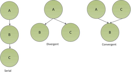
The Bayesian network (Friedman, Geiger, and Goldszmidt 1997) is a graphical model which specifies a factorization of the joint probability distribution (JPD) over a set of variables. The JPD structure is defined by a directed acyclic graph (Atrey, Maddage et al.), in which the nodes represent variables and edges encode independencies between variables (Daoudi, Fohr, and Antoine 2003). A Bayesian network B is defined by a unique JDP over N variables (X₁, X₂, …, X_n) after declaring the conditional independence assumption given by:

(22)

Three variants of the Bayesian network include serial, divergent and convergent, as represented in Figure 5. The naive Bayes classifier, as a special case of Bayesian networks, has received frequent attention for its simplicity and surprisingly good performance. The ability to handle data that are missing during the inference period and training is one of the motivating factors to use Bayesian network classifiers (Cohen et al. 2003). Due to the Bayesian network’s simplicity and linear run-time (Hall 2007), it continues to be a popular learning algorithm for data mining applications. It is suitable for large-scale prediction and classification tasks on complex and incomplete datasets owing to its fast supervised classification.

Figure 5. Basic bayesian network structure.

Multi-class classification (Giannakopoulos et al. 2006), multi-modal input (Prodanov and Drygajlo 2005) and multi-band automatic speech recognition (Daoudi, Fohr, and Antoine 2003) have been proposed to overcome the problems of audio segmentation for movies, error handling in human-robot speech under adverse audio conditions and classical multi-band systems. Bayesian networks are also used to model an extensive variety of phenomena in speech production and recognition (Zweig 2003).

• (f) Linear Discriminant Analysis (LDA)

Linear discriminant analysis (LDA) is a technique for transforming raw data into a new feature space whereby classification can be carried out more robustly (Fisher 1936). If the training set includes M classes, indicates the number of samples in the jth class, is the ith sample of the jth class, and the within-class scatter matrix is given by:

(23)

The between-class scatter matrix is defined as:

(24)

where m denotes the mean of the total dataset.

LDA maximizes the between-class scatter to within-class scatter ratio, which involves maximizing the separation between classes and minimizing the variance within a class (Yang et al. 2013; Ye and Ji 2009). A null space-based LDA (NLDA) (Lu and Wang 2012) was proposed, where in the null space of the within-class scatter matrix the between-class distance is maximized. An LDA-based classifier (Gergen, Nagathil, and Martin 2014) was proposed as a new method to reduce reverberation and interfering sounds in a match between testing and training data when a classifier is trained with clean data. LDA is used to reduce feature dimensions and increase classification accuracy (Lee et al. 2006).

• (g) Support Vector Machines (SVMs)

Support vector machines (SVMs) are evaluated as a useful machine learning technique for solving data classification problems (Vapnik 1998). The goal of SVMs is to obtain the best hyperplane that separates two classes by maximizing the margin among separating boundaries and the closest samples to it (support vector) by implementing a particular training set given by a set (input vector, class)

(25)

where . For a binary classification problem in linearly separable training pairs of two classes, the hyperplane g(x) is given by:

(26)

where are weights and b are biases. The optimal values of and b are obtained by computing the following optimization problem:

(27)

Subject to:

(28)

This equation leads to Lagrange function minimization.

(29)

where the nonzero Lagrange multiplier is .

If two classes are non-linear, Equations (27) and (28) will have different forms and the new function ∅ that should be minimized in 27 is given as:

(30)

(31)

where is the so-called slack variable and C is the upper bound for . By using a kernel trick (Janik and Lobos 2006) to map the training samples from the input vectors to a high-dimensional feature space, SVM finds an optimal separating hyperplane in the feature space and uses a regularization parameter, C, to control model complexity and training error. Several functions including linear, polynomial, sigmoid, and radial basis function (RBF) can be used in SVM (Janik and Lobos 2006). The RBF kernel is applied in SVM to achieve better accuracy than other kernels (Muhammad and Melhem 2014). By learning from training data, SVM achieves the optimum class boundary among the classes (Dhanalakshmi, Palanivel, and Ramalingam 2009). Soft-margin SVM in multi-speaker segmentation separates given points into two target classes, where the SVM uses an upper-bound C to define a hyperplane and improve the SVM (Truong, Lin, and Chen 2007). Several SVM-based classifiers have been developed using clustering schemes based on the confusion matrix to deal with the problems in multi-class classification (Temko and Nadeu 2006) and overlapped sound detection (Temko and Nadeu 2009). In binary classification, the SVM classifier maps the feature vectors into a single binary output (1,−1) using its generalization ability to distinguish auditory brainstem responses (R. Sathya and Abraham 2013) in hearing threshold sensing (Acır, Özdamar et al. 2006). To classify bat call and non-bat events, an SVM-based method combines both temporal and spectral analyses (Andreassen, Surlykke, and Hallam 2014).

• (3) Semi-Supervised Learning Algorithms

A semi-supervised learning algorithm is defined as ‘A process of searching for a suitable classifier from both labeled and unlabeled data.’ An advantage of this methodology is that by utilizing unlabeled data, it provides high classification performance. This methodology facilitates a variety of situations through identifying the specific relationships between labeled and unlabeled data. It also improves unlabeled data by reconstructing the optimal classification boundary (Prakash and Nithya 2014). For instance, graph-based methods are often used as a semi-supervised method. Prakash proposed a graph-based method to define the nodes and edges in a graph. Here nodes are labeled and unlabeled examples in datasets, while edges (potentially weighted) reflect the similarity between samples. Graph approaches are in the form of nonparametric, discriminative, and transductive (Prakash and Nithya 2014). Tianzhu et al. (2012) proposed a new approach where semi-supervised learning takes information according to interesting annotation events in videos from the internet. To handle the difficulties of generic frameworks in various video domains (e.g., sports, news and movies) an algorithm was proposed called Fast Graph-based Semi-supervised multiple instance learning (FGSSMIL). One purpose of this algorithm is to train the models to explore both small-scale expert-labeled and large-scale unlabeled videos. Semi-supervised learning is a possible quantitative tool for comprehending human category learning, in which the majority of input is self-evidently unlabeled. Some popular semi-supervised learning algorithm methods include self-training, co-training, expectation maximization (EM), and transductive support vector machines (Zhu and Goldberg 2009).

1. Self-training

Self-training is one of the popular semi-supervised learning algorithm methods. First, it is specially trained on a small quantity of labeled data, after which it uses a classifier to classify unlabeled data. In the training set, the most confident unlabeled points and their predicted labels are added. This process is repeated by re-training the classifier. The classifier also uses its own predictions to teach itself, which is known as self-teaching or bootstrapping, something different from the statistical procedure with the same name. Sometimes the prediction confidence drops below the threshold level. To solve this problem, a number of algorithms attempt to avoid the ‘unlearn’ unlabeled points (Agrawala 1970). Triguero proposed discriminating the most related filter features in the self-training method from a mixture of an extensive range of noise filters (Triguero et al. 2014). In self-training classification, HMC-SSBR, HMC-SSLP and HMC-SSRAK EL (three new approaches) were proposed to solve the multi-label hierarchical classification problem (Santos and Canuto 2014). A semi-supervised gait recognition algorithm depends on (1) self-training with labeled sequences and (2) a big amount of unlabeled sequences. Self-training classification is useful for improving gait recognition system performance (Yanan et al. 2012).

• (b) Co-Training & Expectation-Maximization

In co-training features are split into two sets. Each feature subset is trained sufficiently by a good classifier (Blum and Mitchell 1998; Mitchell 1999). These two sets are independent conditionally. In the beginning, with the two feature subsets, data are labeled with two separately trained classifiers. Unlabeled data are classified by each classifier. This classifier also teaches the subsequent classifier with the help of some unlabeled samples and predicted labels. This process is repeated by further training the classifier. One of the advantages of unlabeled data is that it reduces the form of space size. A multi-view semi-supervised learning algorithm was proposed to solve the classification issue with sentence boundaries by using lexical and prosodic features (Guz et al. 2010).

The expectation-maximization (EM) algorithm is broadly used as a semi-supervised learning algorithm. It works in different stages (Yunyun, Songcan, and Zhi-Hua 2012). First, it is presented by Dempster (an iterative algorithm), which calculates the maximum likelihood function and estimates the posterior probability distribution under an incomplete sensible circumstance. Dempster is also used for marginal distribution calculation. To reduce the error rate in binary and multi-class classifier problems, an EM-based semi-supervised learning algorithm can be used (Moreno and Agarwal 2003). Yangqiu and Changshui (2008), decreased the labeling work and increased the accuracy rate with a least squares framework used for EM-based semi-supervised learning, which is distance-based music classification. HMM-based large-vocabulary continuous speech recognition (LVCSR) was created to operate multi-view and multi-objective learning for semi-supervised learning algorithms (Cui, Jing, and Jen-Tzung 2012). Yunyun, Songcan, and Zhi-Hua (2012) proposed a new classification algorithm to modify cluster assumption by allowing each instance to be a member of all classes with a corresponding membership. In the learning process information is gained about other members, which is very helpful when the largest memberships are classified with corresponding classes.

• (c) Transductive support vector machines

Transductive support vector machines (TSVMs) are an extension of SVMs with unlabeled data. When SVMs are applied, two matters are considered during classification. First, due to the large numbers of support vectors, SVM classifier complexity can be considerably high during run time. Moreover, unlabeled samples are often more readily available than labeled samples, which are always scarce and expensive to generate. In such conditions, SVM model training time increases as new samples are continually being entered (Guz et al. 2010). To overcome the above problems, Joachims (1999), proposed a TSVM with a semi-supervised learning approach. The purpose of TSVM is to improve the performance of the classifier trained with fewer labeled samples by utilizing unlabeled ones. For automatic AED annotation, Rongyan et al. (2010), applied semi-supervised learning with a TSVM algorithm. TSVM distinguishes between labeled and unlabeled datasets by making boundaries of classes instead of estimating conditional class densities. In this way, it needs considerably less data to perform accurate classification.

Performance evaluation of classification algorithms

AED efficiency is evaluated based on how confident its detection methods are at correct audio detection and accurate classification. According to the nature of any given audio signal, the performance of AED algorithms is both subjectively and objectively evaluated (Arnold 2002). Generally, subjective evaluation is done via a listening test with various decision errors detected based on human perception. On the other hand, objective evaluation is more reliant on mathematical judgment such as true positive, true negative, false positive, and false negative. The True Positive Rate (TPR) calculates the amount of real positives and is precisely recognized as such. The True Negative Rate (TNR) calculates the amount of negatives that are precisely recognized as such. The False Positive Rate (FPR) is specified as the amount of false alarms when an event is incorrectly identified. FPR is also defined as the number of normal events that were misclassified as abnormal events, divided by the total number of normal events. Similarly, the False Negative Rate (FNR) is defined as the proportion of misses. When an event is incorrectly rejected, it is called a miss. As such, FNR can be defined as the total false negatives divided by the total positive instances (Dafna, Tarasiuk, and Zigel. 2013).

The system’s performance is seriously affected by high FPR and FNR, both of which should be minimized along with simultaneously maximizing the true positive (TPR) and true negative (TNR) rates. Both TPR and TNR are based on Equations (1)–(7) and the following measures of performance of audio event detection systems.

(1)

(2)

(3)

(4)

(5)

(6)

(7)

Most systems being studied use similar evaluation metrics, which include detection rate (DR) and false alarm rate (FAR). Other revisions also address problems with AED by offering different metrics to evaluate system efficiency and accuracy. Table 3 provides the proposed evaluation metrics in different AED systems.

Table 3. Evaluation metrics offered in the AED field.

References Accuracy Metrics Description
(Zubair, Yan, and Wang 2013)		● To calculate the classification accuracy; where is the number of correctly classified samples in one class, is the total number of instances and C is the total number of classes.
(Navarathna et al. 2013)		● To calculate speech word recognition accuracy; where N is the number of words, D is the number of deleted words, I is the number of inserted words and S is the number of substitutions.
(Orio 2010)		● To identify the rate and Mean Reciprocal Rank (MRR); where K is the number of identified items and is the position of item k in the rank list returned by the different approaches.
(Temko and Nadeu 2009)		● To detect all instances; where ACC stands for accuracy and AED for audio event detection, and is a weighting factor that balances Precision and Recall. To score an audio segmentation task; where, and are the segment duration, AEs reference number, AEs output number, and number of references, respectively.

Classification approaches

Audio event detection approaches are traditionally studied from two major standpoints: manual and imposed criteria classification. Because it is time consuming, there is no considerable research on these two views. New classification approaches have appeared in event detection with respect to data mining and machine learning algorithms. Pimentel and Clifton divided detection approaches into five separate subcategories, namely probabilistic, distance-based, reconstruction-based, domain-based, and information-theoretic novelty detection (Pimentel et al. 2014). On the other hand, a different approach has been introduced with three clear divisions: unsupervised, supervised, and semi-supervised or fusion. These approaches have been studied distinctly but still suffer from a lack of more detailed and comprehensive research on classification approaches, mainly in audio event detection. This review documents a classification approach with three different subclasses along with a detailed review of each:

• unsupervised learning algorithms;

• supervised learning algorithms; and

• semi-supervised learning algorithms.

We have carefully collected the latest audio event detection methods, specifically those for speech and non-speech event detection (see Table 4). These are not for comparison but as a review of current illustrative approaches. The datasets applying in these researches vary and they come from different resources include public and private or standard datasets. Furthermore, they have different explanations for classification errors.

Table 4. Various audio event detection classification approaches.

Methodology	Ref	Detection approach	No. of articles	Technology type	Detection performance	Type of source
Unsupervised Learning Algorithms	(Pomponi and Vinogradov 2013)	Hierarchical and partition clustering	5	Non-speech	Low	Private Dataset
						3
	(Tsunoo et al. 2011)			Non-speech	Moderate	GTZAN & Ballroom Dataset
	(Lefèvre and Vincent 2011)			Non-speech	Moderate	Private Dataset
	(Yang et al. 2013)			Both	High	SCUTMD movie database
	(Park 2009)			Non-speech	High	Private Dataset
						3
	(Chuan 2013)	GMM	5	Speech	High	Monte Carlo Dataset
	(Choi and Chang 2012)			Both	High	NTT Dataset
	(P. Dhanalakshmi et al. 2011b)			Non-speech	High	Private Dataset
				Non-speech		3
	(Cheng, Sun, and Ji 2010)			Non-speech	High	Private Dataset
						3
	(Chung-Hsien and Chia-Hsin 2006)			Speech	Moderate	Private Dataset
				Speech		3
	(Navarathna et al. 2013)	HMM	7	Speech	Low	AVICAR Dataset
	(Niessen, Van Kasteren, and Merentitis 2013)			Both	Low	IEEE Audio Dataset
						16
	(Itoh, Takiguchi, and Ariki 2013)			Non-speech	Moderate	Private Dataset
	(Wang and Zhang 2012)			Non-speech	Moderate	Private Dataset
	(Milone et al. 2012)			Non-speech	High	Private Dataset
	(Ya-Ti et al. 2009)			Non-speech	Moderate	RWCP Dataset
	(Scheme, Hudgins, and Parker 2007)			Speech	High	Private Dataset
						3
	(P. Dhanalakshmi et al. 2011a)	Neural network (SOM, ART)	3	Both	High	Private Dataset
	(Schroeder et al. 2011)			Non-speech	Moderate	Private Dataset
	(Charalampidis, Georgiopoulos, and Kasparis 2000)			Non-speech	Moderate	Private Dataset
Supervised learning Algorithms	(Khunarsal, Lursinsap, and Raicharoen 2013)	KNN	7	Both	High	BBC and Sound Ideas
	(Ravan and Beheshti 2011)				Moderate	CSLU dataset
	(Liu and Zhang 2012)			Non-speech	Moderate	UCI Dataset
	(Huang et al. 2009)			Non-speech	High	Private Dataset
	(Lie, Hong-Jiang, and Hao 2002)			Non-speech	High	Private Dataset
	(Malhotra, Nikolaidis, and Harms 2008)			Both	High	Private Dataset
	(Balochian, Seidabad, and Rad 2013)	Neural Network (RBF – MLP)	7	Both	High	Private Dataset
	(Ganapathy, Rajan, and Hermansky 2011)			Both	Low	NIST Dataset
	(Mitra and Wang 2008)			Non-speech	High	Private Dataset
	(Kotti et al. 2007)			Speech	High	Private Dataset
	(Shen, Shepherd, and Ngu 2006)			Non-speech	High	GTZAN & Ballroom
	(Turnbull and Elkan 2005)			Non-speech	Low	Private Dataset
	(McConaghy et al. 2003)			Non-speech	High	AN/PPS-15
	(Xu, Zhang, and Liang 2013)	Rule-based	5	Non-speech	High	Private Dataset
	(Ruiz Reyes et al. 2010)			Non-speech	High	Private Dataset
	(Temko, Macho, and Nadeu 2008)			Both	High	CLEAR’07 Dataset
	(Hongwei and Mendel 2007)			Non-speech	High	Private Dataset
	(Yaochu 2000)				Low	Private Dataset
	(Dafna, Tarasiuk, and Zigel. 2013)	Ensemble classifier	4	Non-speech	High	Private Dataset
	(Li, Wang, and Sung 2008)			Non-speech	Moderate	Benchmark Dataset
	(Bin, Haizhou, and Rong 2007)			Speech	Moderate	NIST Dataset
	(Meyer and Schramm 2006)			Speech	High	LVCSR Dataset
	(Giannakopoulos, Pikrakis, and Theodoridis 2007)	Bayesian Network	4	Speech	Moderate	Private Dataset
	(Prodanov and Drygajlo 2005)			Speech	Moderate	RoboX Dataset
	(Daoudi, Fohr, and Antoine 2003)			Speech	Moderate	Private Dataset
	(Zweig 2003)			Speech	Moderate	Private Dataset
	(Gergen, Nagathil, and Martin 2014)	LDA	2	Speech	High	TIMIT Dataset
	(Lee et al. 2006)			Non-speech	High	Private Dataset
	(Andreassen, Surlykke, and Hallam 2014)	SVM	9	Non-speech	High	Private Dataset
	(Muhammad and Melhem 2014)			Speech	High	MEEI Dataset
	(Costa et al. 2012)			Non-speech	Moderate	LMD and ISMIR Dataset
	(Shuiping, Zhenming, and Shiqiang 2011)			Non-speech	High	Private Dataset
	(Dhanalakshmi, Palanivel, and Ramalingam 2009)			Both	High	Private Dataset
	(Temko and Nadeu 2009)			Both	Moderate	CLEAR’07
	(Truong, Lin, and Chen 2007)			Speech	High	public audio Dataset
	(Temko and Nadeu 2006)			Both	High	RWCP Dataset
	(Acır, Özdamar et al. 2006)			Non-speech	High	Private Dataset
Semi-Supervised Learning Algorithms		Self-training, EM, TSVM	8
	(Yanan et al. 2012)			Non-speech	High	Private Dataset
	(Santos and Canuto 2014)			Speech	High	Private Dataset
	(Guz et al. 2010)				Moderate	ICSI MRDA Corpus
	(Cui, Jing, and Jen-Tzung 2012)				High	English broadcast news
	(Rongyan et al. 2010)			Speech	High	Friends melodrama Corpus
	(Yangqiu and Changshui 2008)			Non-speech	Moderate	Private Dataset
	(Moreno and Agarwal 2003)			Speech	High	Linguistic Dataset

Table 4 illustrates existing classification methods based on supervised, unsupervised and semi-supervised learning algorithms. As shown in Table 4, speech and non-speech are two different perceptions of audio signals in audio event detection. In contrast, the performance level is analyzed by grades of high, moderate and low. The sources comprise the datasets available for each method, as elaborated in Table 2. The data are used to differentiate audio features from audio streams and assign them suitable classification. The efficiency of supervised, unsupervised and semi-supervised classification methods is compared based on the accuracy metric and false alarm, particularly in noisy environments. Classification efficiency in supervised learning algorithms indicates performance beyond expectations. The vital aspects of supervised learning algorithms are high accuracy, self-learning, and robustness.

Figure 6 depicts the total number of manuscripts studied over a decade from 2003 to 2014. Although some research have been reported from before the investigated period, research relating to supervised classification methods reached a peak in 2006 and a second peak in 2013 while it was quite stable during the last seven years. It seems this type of classification is still an interesting area for researchers. Likewise, unsupervised classification reached a peak from 2011 to 2013. It did not have very good reputation over the first half of the investigation period but during the second half it was moderately stable. It is not as easy to apply unsupervised classification as it is to apply the supervised method, and it might not be receiving increasing consideration recently. Semi-supervised classification methods were introduced in the middle of the last decade, and based on the report; it has become more interesting lately.

The comparison of technology types according to Table 4 demonstrates a high possibility for researchers to work on the combination area. The report also demonstrates that non-speech has a greater chance of being of primary interest among all three classification categories. Nonetheless, supervised classification researchers are interested in working with a combination of speech and non-speech events as the second choice after speech recognition. Nonetheless, unsupervised classification is not growing at a rate similar to that of speech. In this classification type, non-speech has a greater chance than other technology types. In semi-supervised, the second most interesting area is the non-speech method and researchers are more interested in speech classification, similar to supervised classification.

Unsupervised learning algorithms

Unsupervised learning algorithms comprise an important learning paradigm and have drawn significant attention within the research community as shown by the increasing number of publications in this field. Table 4 lists the most important research works dealing with audio event detection and classification problems related to unsupervised approaches. Developed unsupervised methods for AED are commonly classified into four categories of classifiers. Cluster-based algorithms include a hierarchical or partitioning clustering method (k-means); the neural network-based AEDS comprises the SOM method for unsupervised learning; and finally, the HMM and GMM algorithms are described.

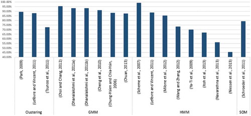
Table 5 illustrates the essential research works using unsupervised learning algorithms to present some solutions to appraise the performance of audio event detection systems with classification techniques. Scheme, Hudgins, and Parker (2007), achieved 91% accuracy with the HMM technique to classify 18 formative phonemes at low noise level (17.5 dB) but when the noise level approached 0 dB the classification accuracy decreased to roughly 38%. Another classification technique (SAP-based GMM) touched accuracy of 95.37% by applying NTT dataset and 14th order MFCC and (SNR = 5 dB), 95.77% (SNR = 10 dB), and 95.75% (SNR = 15 dB) to demonstrate noise classification technique are acceptable in speech enhancement (Choi and Chang 2012). Niessen, Van Kasteren, and Merentitis (2013) also show that meta-classifiers are particularly efficient in combining the stability of several classifiers and also are beneficial on a simple voting scheme. According to the investigated manuscripts, the average accuracy of the unsupervised technique can reach 82.68%, although there are better results in precision or recall evaluation.

Table 5. Evaluation of unsupervised learning algorithms.

Ref	Method	Accuracy rate	Type of input
(Choi and Chang 2012)	To detect speech absence and update the GMM likelihood the speech absence probability (Khunarsal, Lursinsap et al.) is employed.	Accuracy of classification: 95.37%	Speech/Non-Speech
(Navarathna et al. 2013)	Mixture of single audio and four visual streams in a five-stream SHMM	Accuracy of recognition: 56%	Speech
(Scheme, Hudgins, and Parker 2007)	HMM is used to classify words at the phoneme level.	Accuracy of Classification over 91% in low noise	Speech
(Cheng, Sun, and Ji 2010)	MFCC and GMM are used across four passerine species.	Accuracy: 89.1–92.5%	Non-speech
(Milone et al. 2012)	HMM is used to classify acoustic signals	Accuracy of recognition: 85%	Non-speech
(P. Dhanalakshmi et al. 2011b)	Auto-associative neural network model (AANN) combined with a GMM-based classifier	Accuracy of classification: 93%	Non-speech
(Dhanalakshmi, Palanivel et al. 2011a)	Mixture of the auto-associative neural network model (AANN) with GMM	Accuracy of classification: 93.0%	Speech/Non-speech
(Yang et al. 2013)	Spectral clustering and k-means to cluster audio events	Accuracy of detection: %88.63	Speech/Non-speech
(Park 2009)	FCM-DK relies on the fuzzy c-means algorithm that uses a kernel method for data transformation.	Accuracy of classification: 89.12%,	Non-Speech
(Chung-Hsien and Chia-Hsin 2006)	A minimum description length (MDL)-based GMM statistically designates the audio features.	False alarm rate: 0.14 Accuracy of classification: 88%	Speech
(Chuan 2013)	Discrete wavelet transform is used to extract audio features at different scales and time from audio recordings.	Accuracy of classification: 87.32%	Speech/Non-speech
(Niessen, Van Kasteren, and Merentitis 2013)	A hierarchical HMM for sound event detection	F-measure recognition: 45.5%	Speech/Non-speech
(Itoh, Takiguchi, and Ariki 2013)	HMM is used.	Precision: 66.67%, Recall: 100%	Non-Speech
(Wang and Zhang 2012)	HMM mixture to create a framework for ice hockey videos.	Accuracy of HMM 73.01%, Gaussian mixture HMM 59.15%	Non-speech
(Ya-Ti et al. 2009)	A fusion method mixed with hierarchical HMM is employed to cover large differences existing in healthcare audio events.	Accuracy of cassification: 70%	Non-speech
(Schroeder et al. 2011)	Technical method employed in the context of ambient assisted living (AAL).	TPR over 79%, FPR smaller than 4%	Non-speech
(Tsunoo et al. 2011)	K-means algorithm based on one-pass programming.	Accuracy on GTZAN and ballroom dataset 72.4% and 52.5% respectively	Non-speech
(Lefèvre and Vincent 2011)	The proposed method depends on classical HMM, cepstral or spectral analysis and amplitude.	For whistle, crowd and speaker, recall achieved is 95%, 75%, and 95% and precision is 86%, 86%, and 90%	Non-speech

The average of each classification is highlighted in a table within Figure 7 in percentage, Choi and Chang (2012), Scheme, Hudgins, and Parker (2007), Dhanalakshmi et al. (2011b), Dhanalakshmi, Palanivel et al. (2011a) Dhanalakshmi, Palanivel et al. (2011b) reached over 90% accuracy in unsupervised learning algorithms.

Figure 6. Year versus distribution of articles on different classifier types.

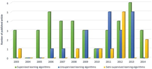
Figure 7. Comparison of unsupervised learning algorithms in terms of accuracy rate.

Supervised learning algorithms

Supervised learning algorithms are characterized as instance-based, neural networks, rule-based, ensemble, Bayesian networks, linear discriminant analysis and support vector machine classifiers. Various supervised learning approaches studied in the context of audio event detection are reviewed under the main category of feature classification. The aim of this literature review is to present supervised learning approaches based on signal classification quality in AED. Audio event classification systems analyze the input audio signal and produces labels that explain the output signal. The most recent experimental research works related to AED employ supervised machine learning algorithms. For more information please see Table 6.

Table 6. Evaluation of supervised learning algorithms.

Ref	Method	Accuracy Rate	Type of input
(Ganapathy, Rajan, and Hermansky 2011)	Speech activity detection (Lin, Li et al.) techniques with an MLP.	Equal error rate: 9%	Speech/Non-speech
(Huang et al. 2009)	K-NN and SVM are employed with three different features to detect frog type	Accuracy: 89.67%	Non-speech
(Xu, Zhang, and Liang 2013)	Wavelet Packet Transform method and Fuzzy SVM	Accuracy of identification: 99%,	Non-speech
(Khunarsal, Lursinsap, and Raicharoen 2013)	Spectrogram pattern matching along with neural network and KNN classifiers	Accuracy: 90.57%.	Speech/Non-speech
(Ravan and Beheshti 2011)	The power spectrum density (PSD) of each speech signal frame is estimated using KNN classification	Accuracy: 90%	Speech
(Liu and Zhang 2012)	New anomaly removal and learning algorithm under the KNN framework	Accuracy: 99.3% when k = 3	Noisy data
(Lie, Hong-Jiang, and Hao 2002)	KNN and linear spectral pairs-vector quantization (LSP-VQ) to discriminate speech from non-speech	Accuracy: over 96%.	Speech/Non-speech
(Balochian, Seidabad, and Rad 2013)	Optimized MLP classifiers to execute some features based on the wavelet transform	Accuracy: 96.49%	Speech/Non-speech
(Kotti et al. 2007)	The cross-correlation function and magnitude of the corresponding cross-power spectral density are fed as input to the neural network for recognition.	Accuracy: 88.1%	Speech
(Shen, Shepherd, and Ngu 2006)	Combination of multiple musical characteristics with a hybrid architecture based on principal component analysis (PCA) and MLP	Accuracy: 91.9%	Non-speech
(Turnbull and Elkan 2005)	Achieved with RBF networks by using a combination of unsupervised and supervised initialization methods	Accuracy: 71.5%	Non-speech
(McConaghy et al. 2003)	RBF algorithms are employed to classify real-life audio radar signals	Accuracy: 86.4%.	Non-speech
(Ruiz Reyes et al. 2010)	Genetic fuzzy system	Accuracy of classification: 97%	Speech/Non-speech
(Temko, Macho, and Nadeu 2008)	Fusion of different information sources with fuzzy integral (FI), fuzzy measure (FM), and SVM	Accuracy 83.9% and precision 81.2%	Speech/Non-speech
(Dafna, Tarasiuk, and Zigel. 2013)	AdaBoost-based algorithms for detection of snore/non-snore	Accuracy of detection: 98.2%	Speech/Non-speech
(Li, Wang, and Sung 2008)	AdaBoostSVM used for sequence of trained RBFSVM classifiers	Accuracy: 85%	Non-speech
(Bin, Haizhou, and Rong 2007)	Ensemble of binary classifiers.	Equal error rate: 1.38% and 3.20%	Speech
(Meyer and Schramm 2006)	AdaBoost.M2 is used for HMM-based speech recognition	Equal error rate: 0.8%	Speech
(Giannakopoulos, Pikrakis, and Theodoridis 2007)	BN in combination with One Versus All classification architecture.	Accuracy: 73.2%, False alarm rate: 11%.	Speech/Non-speech
(Prodanov and Drygajlo 2005)	Bayesian network framework	Accuracy: 77.9%	Speech
(Daoudi, Fohr, and Antoine 2003)	A speech model is built in the time–frequency domain using the formalism of dynamic BNs	Accuracy: 87.89%	Speech
(Zweig 2003)	BNs are used to model a wide variety of phenomena that occur in speech recognition.	Error rate 3.1	Speech
(Gergen, Nagathil, and Martin 2014)	Analyze the influence of reverberation and competing acoustical sources on the classification of audio signals captured by ad hoc distributed microphones	Accuracy: 90%	Speech
(Lee et al. 2006)	UMFCCs and LDA	Accuracy: 96.8% and 98.1%	Non-speech
(Andreassen, Surlykke, and Hallam 2014)	SVM is used based on a combination of temporal and spectral analyses to classify events	Accuracy 96% for dry nights and 70% when raining	Non-speech
(Muhammad and Melhem 2014)	MPEG-7 features are used for indexing, including both video and audio	Accuracy: 99.994%	Non-speech
(Costa et al. 2012)	The audio signal is converted to a spectrogram and features are extracted from time-frequency	Accuracy: 82.33%	Non-speech
(Shuiping, Zhenming, and Shiqiang 2011)	MFFC, ZCR, etc., features are extracted and an audio classification based on SVM was designed	Accuracy: 90%.	Non-speech
(Temko and Nadeu 2009)	SVM-based two-step system outperforms the baseline system for an artificially-generated database	Accuracy: 90.30%	Speech/Non-speech
(Dhanalakshmi, Palanivel, and Ramalingam 2009)	Support vector machines are applied with neural networks (RBFNN)	Accuracy of classification: 92%	Speech/Non-speech
(Truong, Lin, and Chen 2007)	Wavelets and SVMs are employed to segment specific speakers	Accuracy of 94.12% and 85.93% for4-speaker and8-speaker	Speech
(Temko and Nadeu 2006)	Several classifiers based on SVM using confusion matrix-based clustering schemes to deal with multi-class problems	Accuracy 88.29%, average error reduction 31.5%	Non-speech
(Acır, Özdamar et al. 2006)	An SVM classifier is employed with discrete cosine transform (DCT) coefficients and discrete wavelet transform (DWT)	Sensitivity 95.3%, specificity 84.6% and accuracy 93.8%.	Non-speech

Table 6 summarizes the latest methods for tackling audio event detection and classification issues based on supervised learning methods. Statistical comparisons of the accuracy of classifiers trained on specific datasets and false alarm and error rate appraisals are common approaches for comparing supervised learning algorithms (Figure 8). Applying supervised learning algorithms to each classifier results in different accuracy, but in almost all circumstances supervised learning techniques provide high accuracy, precision and recall, and detection rate, reasonable false alarm rates and lower error rates in different groups. The performance synthesis connotes that SVM and ANN are the most valuable supervised classifiers based on investigated manuscripts, but KNN demonstrates better accuracy followed by SVM.

Supervised learning algorithms Xu, Zhang, and Liang (2013), Khunarsal, Lursinsap, and Raicharoen (2013), Ruiz Reyes et al. (2010), Shen, Shepherd, and Ngu (2006), Dafna, Tarasiuk, and Zigel. (2013), Acır, Özdamar et al. (2006), Lee et al. (2006) Andreassen, Surlykke, and Hallam (2014), Lee et al. (2006), Muhammad and Melhem (2014), Dafna, Tarasiuk, and Zigel. (2013), Liu and Zhang (2012), Lie, Hong-Jiang, and Hao (2002), and Balochian, Seidabad, and Rad (2013) touched the highest accuracy over 90% with employing different dataset include public or private. Certainly with different dataset the accuracy of supervised learning algorithms will change therefore comparing different algorithms with different assumption are not accurate.

Semi-supervised learning algorithm

In accordance with the progress made on launching supervised and unsupervised learning algorithms, several semi-supervised learning algorithms have been applied to address scenarios in which the data set is augmented with side information pertaining to the classification of part of the data. Table 7 illustrates the percentage of all research articles implementing semi-supervised learning algorithms.

Table 7. Evaluation of semi-supervised learning algorithms.

Ref	Method	Accuracy Rate	Type of input
(Moreno and Agarwal 2003)	EM-based algorithms for semi-supervised learning with a Gaussian mixture model	Error reduction: 5.04%	Speech
(Cui, Jing, andJen-Tzung 2012)	Cross-view transfer learning for LVCSR through a committee machine	Accuracy: 82.95%	Speech
(Yangqiu and Changshui 2008)	EM algorithm to adaptively learn the fusion scores	Accuracy: 75%	Non-speech
(Rongyan et al. 2010)	TSVM algorithm for automatic AE annotation	Accuracy: 89.6%	Speech/Non-speech
(Guz et al. 2010)	Self-training and co-training classification using lexical and prosodic information	Accuracy: 74.2%	Speech
(Li, Zhang, and Ma 2012)	The CBSL algorithm first selects the sentence level training corpus and then introduces the confirmation criterion to select the word level corpus	Accuracy: 98.83%	Speech
(Yanan et al. 2012)	A semi-supervised gait recognition algorithm based on self-training	Accuracy: 92.4%	Non-speech

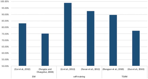
In Table 7, Li, Zhang, and Ma (2012), managed to attain 98.83% classification accuracy using the semi-supervised incremental learning of a large vocabulary continuous speech recognition (LVCSR) system named confirmation-based self-learning (CBSL). Other researchers have proven there is a possibility of over 85% accuracy using the established Gait dataset (Yanan et al. 2012) or TSVM algorithm for automatic AE annotation (Rongyan et al. 2010). But in certain circumstances, even though changing the dataset will not improve the accuracy results and a stable average will be around 60% (Tianzhu et al. 2012). Figure 9 demonstrates the percentage of all research articles that implement semi-supervised learning algorithms.

Figure 8. Comparison of supervised learning algorithms in terms of accuracy rate.

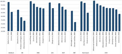
Figure 9. Comparison of semi-supervised learning algorithms in terms of accuracy rate.

Comparative discussion of accuracy rate and false alarm rate evaluation

Theoretically, supervised, unsupervised and semi-supervised learning algorithms only differ in terms of the causal structure of the model. In supervised learning, a qualified person or trained system can properly label the dataset of instances to be used for training. On the other hand, unsupervised learning does not involve labeled data and attempts to find similar patterns in the data to determine the output. Finally, semi-supervised learning is actually a supervised method that avoids labeling a large number of instances. The main objective of AED systems is to maximize classification accuracy and minimize error and false alarm rates. Consequently, the performance of audio event detection schemes for audio signal classification was measured by computing some evaluation metrics, such as classification rates, false alarm rates and error rates for all proposed methods. Table 5, 6, and 7 provide full information on classification and false alarm rates while Figure 9 compares the average accuracy rates of the most popular classification and detection methods.

Figure 10 summarizes the results of different technologies for unsupervised, supervised and semi-supervised classification algorithms, regardless of dataset and environment. The best results are produced by supervised learning algorithms, with an average of 90.13%. The second best results are from semi-supervised methods with 82.99% average followed by 81.07% average for unsupervised methods. GMM is more accurate among unsupervised methods, although Itoh, Takiguchi, and Ariki (2013), demonstrated it is possible to achieve better results in recall with the HMM method. Among supervised methods, the KNN, Adaboost, LDA, SVM and rule-based have shown high output levels; nevertheless, SVM is more interesting for researchers. On the other hand, Xu, Zhang, and Liang (2013), achieved around 99% accuracy demonstrated that the rule-based method is also somewhat capable of achieving one of the best results among supervised methods.

Figure 10. Comparison of supervised, unsupervised and semi-supervised learning algorithms in terms of accuracy rate.

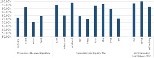
Conclusion and future work

A detailed taxonomy of audio event detection and classification systems was presented in this review. The scope of this review was to analyze researchers’ attempts to explore potential solutions that augment AED. The attempts are expected to maximize audio signal classification accuracy. This review essentially focused on machine learning and classification methods for audio event detection. Throughout this work, published articles related to AED were reviewed, assessed, and grouped into three different trends: unsupervised, supervised, and semi-supervised learning algorithms. A discussion was expanded based on critical comparisons of audio detection methods and algorithms according to accuracy and false alarms by using different datasets. In brief, the classification management techniques can be improved by reducing the false alarm rates, increasing the detection rates and enhancing AED classification accuracy.

There are also recent contributions in deep learning algorithms applied to AED. Some recent representative and significant such results are in publications: Cakir et al. (2015), Parascandolo, Heikki et al. (2016), Gencoglu, Virtanen, and Huttunen (2014), Kumar and Raj (2016), Espi et al. (2015), McLoughlin et al. (2015), Schlüter (2016). In future work, we plan to write a review on deep learning algorithms applied classification of methods in AED.

Abbreviation

Adaptive Boosting	=	AdaBoost
Adaptive resonance theory	=	ART
Artificial neural networks	=	ANNs
Audio event detection	=	AED
Bayesian Networks	=	BNs
Belief-based k-nearest neighbor	=	BK-NN
Confirmation-based self-learning	=	CBSL
Directed acyclic graph	=	DAG
Discrete cosine transform	=	DCT
Discrete Fourier Transform	=	DFT
False Negative Rate	=	FNR
False Positive Rate	=	FPR
Fast Fourier Transform	=	FFT
Fast Graph-based Semi-supervisedmultiple instance learning	=	FGSSMIL
Fuzzy rule-base classifier	=	FRBC
Gaussian Mixture Models	=	GMM
Gaussian mixture models	=	GMMs
Hidden Markov Models	=	HMM
Hierarchical clustering	=	HC
Hierarchical HMMs	=	HHMM
Intelligent surveillance systems	=	ISS
Joint probability distribution	=	JPD
K-nearest neighbor algorithm	=	K-NN
Large vocabulary continuous speech recognition	=	LVCSR
Latent Factor Analysis	=	LFA
Line spectral frequency	=	LSF
Linear Discriminant Analysis	=	LDA
Linear Prediction Coefficients	=	LPC
Linear predictive cepstral coefficient	=	LPCC
Mel-frequency cepstral coefficients	=	MFCCs
Modulation MFCC	=	Mod-MFCC
Multi-layer Perceptron	=	MLP
Mutual k-NN Classifier	=	Mk-NNC
Null space-based LDA	=	NLDA
Perceptual linear prediction	=	PLP
Radial Basis Function	=	RBF
Random forest	=	RF
Self-organizing map	=	SOM
Spectral sub-band centroids	=	SSCs
Support vector machines	=	SVMs
traditional surveillance systems	=	TSS
Transductive support vector machines	=	TSVMs
True Negative Rate	=	TNR
True Positive Rate	=	TPR
Zero-crossing rate	=	ZCR

References

- Acır, N., Ö. Özdamar, and C. Güzeliş. 2006. Automatic classification of auditory brainstem responses using SVM-based feature selection algorithm for threshold detection. Engineering Applications of Artificial Intelligence 19 (2):209–18.
- Agrawala, A. 1970. Learning with a probabilistic teacher. IEEE Transactions on Information Theory 16 (4):373–79.
- Alcala-Fdez, J., R. Alcala, and F. Herrera. 2011. A fuzzy association rule-based classification model for high-dimensional problems with genetic rule selection and lateral tuning. IEEE Transactions on Fuzzy Systems 19 (5):857–72.
- Andreassen, T., A. Surlykke, and J. Hallam. 2014. Semi-automatic long-term acoustic surveying: A case study with bats. Ecological Informatics 21:13–24.
- Arnold, M. 2002. Subjective and objective quality evaluation of watermarked audio tracks. Proceedings. Second International Conference on Web Delivering of Music. WEDELMUSIC. IEEE.
- Atrey, P. K., M. C. Maddage, and M. S. Kankanhalli. 2006. Audio based event detection for multimedia surveillance. International Conference on Acoustics, Speech and Signal Processing, ICASSP Proceedings, IEEE.
- Bailey, T., and A. K. Jain. 1978. A note on distance-weighted k-nearest neighbor rules. IEEE Transactions on Systems, Man and Cybernetics 8 (4):311–13.
- Balochian, S., E. A. Seidabad, and S. Z. Rad. 2013. Neural network optimization by genetic algorithms for the audio classification to speech and music. International Journal of Signal Processing, Image Processing & Pattern Recognition 6 (3).
- Bardeli, R., D. Wolff, F. Kurth, M. Koch, K. H. Tauchert, and K. H. Frommolt. 2010. Detecting bird sounds in a complex acoustic environment and application to bioacoustic monitoring. Pattern Recognition Letters 31 (12):1524–34.
- Bauer, E., and R. Kohavi. 1999. An empirical comparison of voting classification algorithms: Bagging, boosting, and variants. Machine Learning 36 (1–2):105–39.
- Baum, L. E., and T. Petrie. 1966. Statistical inference for probabilistic functions of finite state Markov chains. The Annals of Mathematical Statistics 37 (6):1554–63.
- Besacier, L., J. F. Bonastre, and C. Fredouille. 2000. Localization and selection of speaker-specific information with statistical modeling. Speech Communication 31 (2–3):89–106.
- Bhatia, N. 2010. Survey of nearest neighbor techniques. International Journal of Computer Science and Information Security (IJCSIS) 8 (2):302–305.
- Bhavsar, H., and A. Ganatra. 2012. A comparative study of training algorithms for supervised machine learning. International Journal of Soft Computing and Engineering (IJSCE) 2 (4):2231–2307.
- Bin, M., L. Haizhou, and T. Rong. 2007. Spoken language recognition using ensemble classifiers. IEEE Transactions on Audio, Speech, and Language Processing 15 (7):2053–62.
- Blum, A., and T. Mitchell. 1998. Combining labeled and unlabeled data with co-training. Proceedings of the eleventh annual conference on Computational learning theory, ACM.
- Bourlard, H. A., and N. Morgan. 1993. Connectionist speech recognition: A hybrid approach. Kluwer Academic Publishers. https://link.springer.com/book/10.1007%2F978-1-4615-3210-1
- Breiman, L. 1996. Bagging predictors. Machine Learning 24 (2):123–40.
- Breiman, L. 2001. Random forests. Machine Learning 45 (1):5–32.
- Buckley, J. J., and Y. Hayashi. 1994. Fuzzy genetic algorithm and applications. Fuzzy Sets and Systems 61 (2):129–36.
- Busso, C., S. Lee, and S. Narayanan. 2009. Analysis of emotionally salient aspects of fundamental frequency for emotion detection. IEEE Transactions on Audio, Speech, and Language Processing 17 (4):582–96.
- Cakir, E., T. Heittola, H. Huttunen, and T. Virtanen. 2015. Polyphonic sound event detection using multi label deep neural networks. Neural Networks (IJCNN), 2015 International Joint Conference on, IEEE. pp. 1–7.
- Campbell, J. P., Jr. 1997. Speaker recognition: A tutorial. Proceedings of the IEEE 85 (9):1437–62.
- Carpenter, G. A., S. Grossberg, and J. H. Reynolds. 1991. ARTMAP: Supervised real-time learning and classification of nonstationary data by a self-organizing neural network. Neural Networks 4 (5):565–88.
- Charalampidis, D., M. Georgiopoulos, and T. Kasparis. 2000. Classification of noisy signal using fuzzy ARTMAP neural networks. International Joint Conference on Neural Networks, IJCNN2000, Proceedings of the IEEE-INNS-ENNS.
- Cheng, J., Y. Sun, and L. Ji. 2010. A call-independent and automatic acoustic system for the individual recognition of animals: A novel model using four passerines. Pattern Recognition 43 (11):3846–52.
- Choi, J.-H., and J.-H. Chang. 2012. On using acoustic environment classification for statistical model-based speech enhancement. Speech Communication 54 (3):477–90.
- Chuan, C.-H. 2013. Audio classification and retrieval using wavelets and gaussian mixture models. International Journal Multimed Data Engineering Managed 4 (1):1–20.
- Chung-Hsien, W., and H. Chia-Hsin. 2006. Multiple change-point audio segmentation and classification using an MDL-based Gaussian model. IEEE Transactions on Audio, Speech, and Language Processing 14 (2):647–57.
- Cintra, M. E., M. C. Monard, E. A. Cherman, and H. De Arruda Camargo. 2011. On the estimation of the number of fuzzy sets for fuzzy rule-based classification systems. 11th International Conference on Hybrid Intelligent Systems (HIS), 2011.
- Clavel, C., T. Ehrette, and G. Richard. 2005. Events detection for an audio-based surveillance system. IEEE International Conference on Multimedia and Expo, 2005. ICME 2005.
- Cohen, I., N. Sebe, F. G. Gozman, M. C. Cirelo, and T. S. Huang. 2003. Learning Bayesian network classifiers for facial expression recognition both labeled and unlabeled data. IEEE Computer Society Conference on Computer Vision and Pattern Recognition, 2003. Proceedings.
- Cordón, O., M. J. Del Jesus, and F. Herrera. 1999. A proposal on reasoning methods in fuzzy rule-based classification systems. International Journal of Approximate Reasoning 20 (1):21–45.
- Costa, Y. M. G., L. S. Oliveira, A. L. Koerich, F. Gouyon, and J. G. Martins. 2012. Music genre classification using LBP textural features. Signal Processing 92 (11):2723–37.
- Cover, T., and P. Hart. 1967. Nearest neighbor pattern classification. IEEE Transactions on Information Theory 13 (1):21–27.
- Cui, X., H. Jing, and C. Jen-Tzung. 2012. Multi-view and multi-objective semi-supervised learning for HMM-based automatic speech recognition. IEEE Transactions on Audio, Speech, and Language Processing 20 (7):1923,1935.
- Dafna, E., A. Tarasiuk, and Y. Zigel. 2013. Automatic detection of whole night snoring events using non-contact microphone. PLoS One 8 (12). doi:10.1371/journal.pone.0084139
- Damper, R. I., and J. E. Higgins. 2003. Improving speaker identification in noise by subband processing and decision fusion. Pattern Recognition Letters 24 (13):2167–73.
- Daoudi, K., D. Fohr, and C. Antoine. 2003. Dynamic Bayesian networks for multi-band automatic speech recognition. Computer Speech & Language 17 (2–3):263–85.
- Davis, S. B., and P. Mermelstein. 1980. Comparison of parametric representations for monosyllabic word recognition in continuously spoken sentences. IEEE Transactions on Acoustics, Speech and Signal Processing 28 (4):357–66.
- Deller, J. J. R., J. H. L. Hansen, and J. G. Proakis. (2000). Discrete-Time Processing of Speech Signals. Hoboken, New Jersey, USA: Wiley-IEEE Press.
- Dhanalakshmi, P., S. Palanivel, and V. Ramalingam. 2009. Classification of audio signals using SVM and RBFNN. Expert Systems with Applications 36 (3):6069–75.
- Dhanalakshmi, P., S. Palanivel, and V. Ramalingam. 2011a. Classification of audio signals using AANN and GMM. Applied Soft Computing 11 (1):716–23.
- Dhanalakshmi, P., S. Palanivel, and V. Ramalingam. 2011b. Pattern classification models for classifying and indexing audio signals. Engineering Applications of Artificial Intelligence 24 (2):350–57.
- Dietterich, T. 2000a. Ensemble methods in machine learning. Multiple Classifier Systems, Springer Berlin Heidelberg 1857:1–15.
- Dietterich, T. 2000b. An experimental comparison of three methods for constructing ensembles of decision trees: Bagging, boosting, and randomization. Machine Learning 40 (2):139–57.
- Driggers, R. G. 2003. Encyclopedia of Optical Engineering (Vol. 3). Maryland, USA: Marcel Dekker Inc.
- Drugman, T. 2014. Using mutual information in supervised temporal event detection: Application to cough detection. Biomedical Signal Processing and Control 10:50–57.
- Espi, M., M. Fujimoto, K. Kinoshita, and T. Nakatani. 2015. Exploiting spectro-temporal locality in deep learning based acoustic event detection. EURASIP Journal on Audio, Speech, and Music Processing 2015 (26): 1–12.
- Fisher, R. A. 1936. The use of multiple measurements in taxonomic problems. Annals of Eugenics 7 (2):179–88.
- Freund, Y., and R. E. Schapire. 1996. Experiments with a new boosting algorithm. ICML, Bari, Italy Morgan Kaufmann Publishers Inc.San Francisco, CA, USA.
- Freund, Y., and R. E. Schapire. 1997. A decision-theoretic generalization of on-line learning and an application to boosting. Journal of Computer and System Sciences 55 (1):119–39.
- Friedman, N., D. Geiger, and M. Goldszmidt. 1997. Bayesian network classifiers. Machine Learning 29 (2–3):131–63.
- Ganapathy, S., P. Rajan, and H. Hermansky. 2011. Multi-layer perceptron based speech activity detection for speaker verification. IEEE Workshop on Applications of Signal Processing to Audio and Acoustics (WASPAA).
- Gencoglu, O., T. Virtanen, and H. Huttunen. 2014. Recognition of acoustic events using deep neural networks. Signal Processing Conference (EUSIPCO), 2014 Proceedings of the 22nd European, IEEE, pp. 506–10.
- Gergen, S., A. Nagathil, and R. Martin. 2014. Classification of reverberant audio signals using clustered ad hoc distributed microphones. Signal Processing 107:21–32.
- Giannakopoulos, T., D. Kosmopoulos, A. Aristidou, and S. Theodoridis. 2006. Violence content classification using audio features. Advances in Artificial Intelligence, Berlin, Heidelberg: Springer, 502–07.
- Giannakopoulos, T., and A. Pikrakis. 2014. Chapter 4 - audio features. In Introduction to audio analysis, Eds. T. Giannakopoulos, and A. Pikrakis, 59–103. Oxford: Academic Press.
- Giannakopoulos, T., A. Pikrakis, and S. Theodoridis. 2007. A multi-class audio classification method with respect to violent content in movies using bayesian networks. Multimedia Signal Processing, 2007. MMSP 2007. IEEE 9th Workshop on.
- Grossberg, S. 1976. Adaptive pattern classification and universal recoding: II. Feedback, expectation, olfaction, illusions. Biological Cybernetics 23 (4):187–202.
- Guz, U., S. Cuendet, D. Hakkani-Tür, and G. Tur. 2010. Multi-view semi-supervised learning for dialog act segmentation of speech. IEEE Transactions on Audio, Speech, and Language Processing 18 (2):320,329.
- Hall, M. 2007. A decision tree-based attribute weighting filter for naive Bayes. Knowledge-Based Systems 20 (2):120–26.
- Hermansky, H. 1990. Perceptual linear predictive (PLP) analysis of speech. The Journal of the Acoustical Society of America 87 (4):1738–52.
- Hongwei, W., and J. M. Mendel. 2007. Classification of battlefield ground vehicles using acoustic features and fuzzy logic rule-based classifiers. IEEE Transactions on Fuzzy Systems 15 (1):56–72.
- Huang, C.-J., Y.-J. Yang, D.-X. Yang, and Y.-J. Chen. 2009. Frog classification using machine learning techniques. Expert Systems with Applications 36 (2, Part 2):3737–43.
- Itoh, H., T. Takiguchi, and Y. Ariki. 2013. Event detection and recognition using HMM with whistle sounds. Signal-Image Technology & Internet-Based Systems (SITIS), 2013 International Conference on.
- Jain, A. K., R. P. W. Duin, and M. Jianchang. 2000. Statistical pattern recognition: A review. IEEE Transactions on Pattern Analysis and Machine Intelligence 22 (1):4–37.
- Janik, P., and T. Lobos. 2006. Automated classification of power-quality disturbances using SVM and RBF networks. IEEE Transactions on Power Delivery 21 (3):1663–69.
- Joachims, T. 1999. Transductive inference for text classification using support vector machines. ICML, Morgan Kaufmann Publishers Inc. San Francisco, CA, USA.
- Kalteh, A. M., P. Hjorth, and R. Berndtsson. 2008. Review of the self-organizing map (SOM) approach in water resources: Analysis, modelling and application. Environmental Modelling & Software 23 (7):835–45.
- Kaufman, L., and P. J. Rousseeuw. 1990. Finding groups in data: An introduction to cluster analysis. New York: Wiley.
- Khairnar, D. G., S. N. Merchant, and U. B. Desai. 2005. An optimum RBF network for signal detection in non-gaussian noise. In Pattern recognition and machine intelligence, Eds. S. Pal, S. Bandyopadhyay, and S. Biswas, Springer Berlin Heidelberg, 3776:306–309.
- Khunarsal, P., C. Lursinsap, and T. Raicharoen. 2013. Very short time environmental sound classification based on spectrogram pattern matching. Information Sciences 243:57–74.
- Kinnunen, T., and H. Li. 2010. An overview of text-independent speaker recognition: From features to supervectors. Speech Communication 52 (1):12–40.
- Kinnunen, T., I. Sidoroff, M. Tuononen, and P. Fränti. 2011. Comparison of clustering methods: A case study of text-independent speaker modeling. Pattern Recognition Letters 32 (13):1604–17.
- Kinnunen, T., B. Zhang, J. Zhu, and Y. Wang. 2007. Speaker verification with adaptive spectral subband centroids. In Advances in biometrics, Eds. S.-W. Lee, and S. Li, Springer Berlin Heidelberg, 4642: 58–66.
- Kohonen, T. 1982. Analysis of a simple self-organizing process. Biological Cybernetics 44 (2):135–40.
- Kotti, M., E. Benetos, C. Kotropoulos, and I. Pitas. 2007. A neural network approach to audio-assisted movie dialogue detection. Neurocomputing 71 (1–3):157–66.
- Kulkarni, V. Y., and P. K. Sinha. 2013. Random forest classifiers: A survey and future research directions. Int Journal of Advanced Computing 36 (1):1144–53.
- Kumar, A., and B. Raj. 2016. Audio event detection using weakly labeled data. Proceedings of the 2016 ACM on Multimedia Conference, ACM, pp. 1038–47.
- Lamel, L., L. Rabiner, A. E. Rosenberg, and J. G. Wilpon. 1981. An improved endpoint detector for isolated word recognition. IEEE Transactions on Acoustics, Speech and Signal Processing 29 (4):777–85.
- Larsen, B., and C. Aone. 1999. Fast and effective text mining using linear-time document clustering. Proceedings of the fifth ACM SIGKDD international conference on Knowledge discovery and data mining, ACM.
- Lee, C.-H., C.-H. Chou, -C.-C. Han, and R.-Z. Huang. 2006. Automatic recognition of animal vocalizations using averaged MFCC and linear discriminant analysis. Pattern Recognition Letters 27 (2):93–101.
- Lefèvre, S., and N. Vincent. 2011. A two level strategy for audio segmentation. Digital Signal Processing 21 (2):270–77.
- Li, D., I. K. Sethi, N. Dimitrova, and T. McGee. 2001. Classification of general audio data for content-based retrieval. Pattern Recognition Letters 22 (5):533–44.
- Li, H., T. Zhang, and L. Ma. 2012. Confirmation based self-learning algorithm in LVCSR’s semi-supervised incremental learning. Procedia Engineering 29:754–59.
- Li, L., G. Fengpei, Z. Qingwei, and Y. Yonghong. 2010. Detecting cheering events in sports games. 2nd International Conference on Education Technology and Computer (ICETC).
- Li, X., L. Wang, and E. Sung. 2008. AdaBoost with SVM-based component classifiers. Engineering Applications of Artificial Intelligence 21 (5):785–95.
- Lie, L., Z. Hong-Jiang, and J. Hao. 2002. Content analysis for audio classification and segmentation. IEEE Transactions on Speech and Audio Processing 10 (7):504–16.
- Lin, L., Y. Li, and A. Sadek. 2013. A k nearest neighbor based local linear wavelet neural network model for on-line short-term traffic volume prediction. Procedia - Social and Behavioral Sciences 96:2066–77.
- Liu, H., and S. Zhang. 2012. Noisy data elimination using mutual k-nearest neighbor for classification mining. Journal of Systems and Software 85 (5):1067–74.
- Liu, Z.-G., Q. Pan, and J. Dezert. 2013. A new belief-based K-nearest neighbor classification method. Pattern Recognition 46 (3):834–44.
- Lu, G. 2001. Indexing and retrieval of audio: A survey. Multimedia Tools and Applications 15 (3):269–90.
- Lu, G.-F., and Y. Wang. 2012. Feature extraction using a fast null space based linear discriminant analysis algorithm. Information Sciences 193:72–80.
- Malhotra, B., I. Nikolaidis, and J. Harms. 2008. Distributed classification of acoustic targets in wireless audio-sensor networks.”. Computation Network 52 (13):2582–93.
- Mayer, R., R. Neumayer, D. Baum, and A. Rauber. 2009. Analytic comparison of self-organising maps. In Advances in self-organizing maps, Eds. J. Príncipe, and R. Miikkulainen, Springer Berlin Heidelberg, 5629: 182–190.
- McConaghy, T., H. Leung, E. Bosse, and V. Varadan. 2003. Classification of audio radar signals using radial basis function neural networks. IEEE Transactions on Instrumentation and Measurement 52 (6):1771–79.
- McLoughlin, I., H. Zhang, Z. Xie, Y. Song, and W. Xiao. 2015. Robust sound event classification using deep neural networks. IEEE/ACM Transactions on Audio, Speech, and Language Processing 23 (3):540–52.
- Meyer, C., and H. Schramm. 2006. Boosting HMM acoustic models in large vocabulary speech recognition. Speech Communication 48 (5):532–48.
- Milone, D. H., J. R. Galli, C. A. Cangiano, H. L. Rufiner, and E. A. Laca. 2012. Automatic recognition of ingestive sounds of cattle based on hidden Markov models. Computers and Electronics in Agriculture 87:51–55.
- Mitchell, T. 1999. The role of unlabeled data in supervised learning. Proceedings of the sixth international colloquium on cognitive science, Citeseer.
- Mitra, V., and C.-J. Wang. 2008. Content based audio classification: A neural network approach. Soft Computing 12 (7):639–46.
- Moreno, P. J., and S. Agarwal. 2003. An experimental study of EM-based algorithms for semi-supervised learning in audio classification. ICML 2003 Workshop on the Continuum from Labeled to Unlabeled Data in Machine Learning and Data Mining.
- Muhammad, G., and M. Melhem. 2014. Pathological voice detection and binary classification using MPEG-7 audio features. Biomedical Signal Processing and Control 11:1–9.
- Muñoz-Expósito, J. E., S. García-Galán, N. Ruiz-Reyes, and P. Vera-Candeas. 2007. Adaptive network-based fuzzy inference system vs. other classification algorithms for warped LPC-based speech/music discrimination. Engineering Applications of Artificial Intelligence 20 (6):783–93.
- Navarathna, R., D. Dean, S. Sridharan, and P. Lucey. 2013. Multiple cameras for audio-visual speech recognition in an automotive environment. Computer Speech & Language 27 (4):911–27.
- Neiberg, D., G. Salvi, and J. Gustafson. 2013. Semi-supervised methods for exploring the acoustics of simple productive feedback. Speech Communication 55 (3):451–69.
- Niessen, M. E., T. L. M. Van Kasteren, and A. Merentitis. 2013. Hierarchical modeling using automated sub-clustering for sound event recognition. IEEE Workshop on Applications of Signal Processing to Audio and Acoustics (WASPAA).
- Nillson, N. 1965. Learning machines: Foundations of trainable pattern classifying systems. New York: McGraw-Hill.
- Nirmal, J., S. Patnaik, M. Zaveri, and P. Kachare. 2013. Multi-scale speaker transformation using radial basis function. Procedia Technology 10:311–19.
- Nozaki, K., H. Ishibuchi, and H. Tanaka. 1996. Adaptive fuzzy rule-based classification systems. IEEE Transactions on Fuzzy Systems 4 (3):238–50.
- Oppenheim, A. V., R. W. Schafer, and J. R. Buck. 1989. Discrete-time signal processing. Englewood Cliffs: Prentice-hall.
- Orio, N. 2010. Automatic identification of audio recordings based on statistical modeling. Signal Processing 90 (4):1064–76.
- Parascandolo, G., H. Huttunen, and T. Virtanen. 2016. Recurrent neural networks for polyphonic sound event detection in real life recordings. Acoustics, Speech and Signal Processing (ICASSP), 2016 IEEE International Conference on, IEEE, pp. 6440–44.
- Park, D.-C. 2009. Classification of audio signals using Fuzzy c-means with divergence-based Kernel. Pattern Recognition Letters 30 (9):794–98.
- Pellegrini, T., J. Portêlo, I. Trancoso, A. Abad, and M. Bugalho. 2009. Hierarchical clustering experiments for application to audio event detection. Proceedings of the 13th International Conference on Speech and Computer.
- Pimentel, M. A. F., D. A. Clifton, L. Clifton, and L. Tarassenko. 2014. A review of novelty detection. Signal Processing 99:215–49.
- Polikar, R., L. Upda, S. S. Upda, and V. Honavar. 2001. Learn++: An incremental learning algorithm for supervised neural networks. IEEE Transactions on Systems, Man, and Cybernetics, Part C: Applications and Reviews 31 (4):497–508.
- Pomponi, E., and A. Vinogradov. 2013. A real-time approach to acoustic emission clustering. Mechanical Systems and Signal Processing 40 (2):791–804.
- Potamitis, I., S. Ntalampiras, O. Jahn, and K. Riede. 2014. Automatic bird sound detection in long real-field recordings: Applications and tools. Applied Acoustics 80:1–9.
- Prakash, V. J., and D. L. Nithya. 2014. A survey on semi-supervised learning techniques. International Journal of Computer Trends and Technology (IJCTT) 8(1):25–29.
- Principe, J. C., N. R. Euliano, and W. C. Lefebvre. 2000. Neural and adaptive systems: Fundamentals through simulations. New York: Wiley.
- Prodanov, P., and A. Drygajlo. 2005. Bayesian networks based multi-modality fusion for error handling in human–Robot dialogues under noisy conditions. Speech Communication 45 (3):231–48.
- Qiang, H., and S. Cox. 2011. Inferring the structure of a tennis game using audio information. IEEE Transactions on Audio, Speech, and Language Processing 19 (7):1925–37.
- Radhakrishnan, R., A. Divakaran, and P. Smaragdis. 2005. Audio analysis for surveillance applications. Applications of Signal Processing to Audio and Acoustics, 2005. IEEE Workshop on.
- Ravan, M., and S. Beheshti. 2011. Speech recognition from adaptive windowing PSD estimation. 24th Canadian Conference on Electrical and Computer Engineering (CCECE), 524–27.
- Reaves, B. 1991. Comments on “An improved endpoint detector for isolated word recognition. Signal Processing, IEEE Transactions On 39 (2):526–27.
- Reynolds, D. A. 1995. Speaker identification and verification using Gaussian mixture speaker models. Speech Communication 17 (1–2):91–108.
- Reynolds, D. A., T. F. Quatieri, and R. B. Dunn. 2000. Speaker verification using adapted gaussian mixture models. Digital Signal Processing 10 (1–3):19–41.
- Rojek, I., M. Jagodziński, et al. 2012. Hybrid artificial intelligence system in constraint based scheduling of integrated manufacturing ERP systems. In Hybrid artificial intelligent systems, Eds. E. Corchado, V. Snášel, and A. Abraham, Springer Berlin Heidelberg, 7209: 229–240.
- Rokach, L. 2009. Taxonomy for characterizing ensemble methods in classification tasks: A review and annotated bibliography. Computational Statistics & Data Analysis 53 (12):4046–72.
- Rongyan, W., L. Gang, G. Jun, and M. Zhenxin. 2010. Semi-supervised learning for automatic audio events annotation using TSVM. International Conference on Computer Application and System Modeling (ICCASM).
- Ruiz Reyes, N., P. Vera Candeas, S. García Galán, and J. E. Muñoz. 2010. Two-stage cascaded classification approach based on genetic fuzzy learning for speech/music discrimination. Engineering Applications of Artificial Intelligence 23 (2):151–59.
- Santos, A., and A. Canuto. 2014. Applying semi-supervised learning in hierarchical multi-label classification. Expert Systems with Applications 41(14): 6075–6085.
- Sathya, R., and A. Abraham. 2013. Comparison of supervised and unsupervised learning algorithms for pattern classification. (IJARAI) International Journal of Advanced Research in Artificial Intelligence 2 (2). http://thesai.org/Publications/ViewPaper?Volume=2&Issue=2&Code=IJARAI&SerialNo=6
- Scheme, E. J., B. Hudgins, and P. A. Parker. 2007. Myoelectric signal classification for phoneme-based speech recognition. IEEE Transactions on Biomedical Engineering 54 (4):694–99.
- Schlüter, J. 2016.Learning to pinpoint singing voice from weakly labeled examples. Proceedings of the International Society for Music Information Retrieval Conference (ISMIR), pp. 44–50.
- Schölkopf, B., A. Smola, and K.-R. Müller. 1998. Nonlinear component analysis as a kernel eigenvalue problem. Neural Computation 10 (5):1299–319.
- Schroeder, J., S. Wabnik, P. J. Hengel, and S. Goetze. 2011. Detection and classification of acoustic events for in-home care. In Ambient assisted living, Eds. R. Wichert, and B. Eberhardt, Springer Berlin Heidelberg, 181–195.
- Schuller, B., A. Batliner, S. Steidl, and D. Seppi. 2011. Recognising realistic emotions and affect in speech: State of the art and lessons learnt from the first challenge. Speech Communication 53 (9–10):1062–87.
- Schwarz, P., P. Matejka, and J. Cernocky. 2006. Hierarchical structures of neural networks for phoneme recognition. IEEE International Conference on Acoustics, Speech and Signal Processing. ICASSP 2006 Proceedings.
- Sharma, S., and R. Lal Yadav. 2013. Comparative study of K-means and robust clustering. International Journal of Advanced Computer Research 3 (12):207–210.
- Shen, J., J. Shepherd, and A. H. H. Ngu. 2006. Towards effective content-based music retrieval with multiple acoustic feature combination. IEEE Transactions on Multimedia 8 (6):1179–89.
- Shuiping, W., T. Zhenming, and L. Shiqiang. 2011. Design and implementation of an audio classification system based on SVM. Procedia Engineering 15:4031–35.
- Skurichina, M., and R. P. W. Duin. 2002. Bagging, boosting and the random subspace method for linear classifiers. Pattern Analysis & Applications 5 (2):121–35.
- Stavrakoudis, D. G., I. Z. Gitas, and J. B. Theocharis. 2011. A hierarchical genetic fuzzy rule-based classifier for high-dimensional classification problems. IEEE International Conference on Fuzzy Systems (FUZZ).
- Sturim, D. E., P. A. Torres-Carrasquillo, T. F. Quatieri, N. Malyska, and A. McCree. 2011. Automatic detection of depression in speech using gaussian mixture modeling with factor analysis. Interspeech, Florence, Italy, ISCA.
- Su, P.-C., C.-H. Lan, C.-S. Wu, Z.-X. Zeng, and W.-Y. Chen. 2013. Transition effect detection for extracting highlights in baseball videos. EURASIP Journal on Image and Video Processing 2013 (1):1–16.
- Sun, Y., S. Todorovic, and J. Li. 2006. Reducing the overfitting of AdaBoost by controlling its data distribution skewness. International Journal of Pattern Recognition and Artificial Intelligence 20 (07):1093–116.
- Tao, C. W. 2002. A reduction approach for fuzzy rule bases of fuzzy controllers. IEEE Transactions on Systems, Man, and Cybernetics, Part B: Cybernetics 32 (5):668–75.
- Temko, A., D. Macho, and C. Nadeu. 2008. Fuzzy integral based information fusion for classification of highly confusable non-speech sounds. Pattern Recognition 41 (5):1814–23.
- Temko, A., and C. Nadeu. 2006. Classification of acoustic events using SVM-based clustering schemes. Pattern Recognition 39 (4):682–94.
- Temko, A., and C. Nadeu. 2009. Acoustic event detection in meeting-room environments. Pattern Recognition Letters 30 (14):1281–88.
- Tianzhu, Z., X. Changsheng, Z. Guangyu, L. Si, and L. Hanqing. 2012. A generic framework for video annotation via semi-supervised learning. IEEE Transactions on Multimedia 14 (4):1206–19.
- Tin Kam, H. 1998. The random subspace method for constructing decision forests. IEEE Transactions on Pattern Analysis and Machine Intelligence 20 (8):832–44.
- Tong, Z., and C. C. J. Kuo. 2001. Audio content analysis for online audiovisual data segmentation and classification. IEEE Transactions on Speech and Audio Processing 9 (4):441–57.
- Triguero, I., J. A. Sáez, J. Luengo, S. García, and F. Herrera. 2014. On the characterization of noise filters for self-training semi-supervised in nearest neighbor classification. Neurocomputing 132:30–41.
- Truong, T. K., -C.-C. Lin, and S.-H. Chen. 2007. Segmentation of specific speech signals from multi-dialog environment using SVM and wavelet. Pattern Recognition Letters 28 (11):1307–13.
- Tsunoo, E., G. Tzanetakis, N. Ono, and S. Sagayama. 2011. Beyond timbral statistics: Improving music classification using percussive patterns and bass lines. IEEE Transactions on Audio, Speech, and Language Processing 19 (4):1003–14.
- Turnbull, D., and C. Elkan. 2005. Fast recognition of musical genres using RBF networks. IEEE Transactions on Knowledge and Data Engineering 17 (4):580–84.
- Tzortzis, G., and A. Likas. 2008. The global kernel k-means clustring algorithm. IEEE International Joint Conference on Neural Networks, 2008. IJCNN 2008. (IEEE World Congress on Computational Intelligence), IEEE.
- Uncini, A. 2003. Audio signal processing by neural networks. Neurocomputing 55 (3–4):593–625.
- Vapnik, V. 1998. Statistical learning theory. New York: Wiley.
- Wang, X., and X.-P. Zhang. 2012. Ice hockey shooting event modeling with mixture hidden Markov model. Multimedia Tools and Applications 57 (1):131–44.
- Weimin, H., C. Tuan-Kiang, L. Haizhou, K. Tian Shiang, and J. Biswas. 2010. Scream detection for home applications. 5th IEEE Conference on Industrial Electronics and Applications (ICIEA).
- Xiaodan, Z., H. Jing, G. Potamianos, and M. Hasegawa-Johnson. 2009. Acoustic fall detection using Gaussian mixture models and GMM supervectors. IEEE international conference on acoustics. Speech and Signal Processing, 2009. ICASSP 2009.
- Xu, Q., L. Zhang, and W. Liang. 2013. Acoustic detection technology for gas pipeline leakage. Process Safety and Environmental Protection 91 (4):253–61.
- Yanan, L., Y. Yilong, L. Lili, P. Shaohua, and Y. Qiuhong. 2012. Semi-supervised gait recognition based on self-training. IEEE Ninth International Conference on Advanced Video and Signal-Based Surveillance (AVSS), 2012.
- Yang, J.-C., L.-A. Liu, Q.-W. Qin, and M. Zhang. 2013. Audio event change detection and clustering in movies. Journal of Multimedia 8 (2):113–20.
- Yangqiu, S., and Z. Changshui. 2008. Content-based information fusion for semi-supervised music genre classification. IEEE Transactions on MultiMedia 10 (1):145–52.
- Yaochu, J. 2000. Fuzzy modeling of high-dimensional systems: Complexity reduction and interpretability improvement. IEEE Transactions on Fuzzy Systems 8 (2):212–21.
- Ya-Ti, P., L. Ching-Yung, S. Ming-Ting, and T. Kun-Cheng. 2009. Healthcare audio event classification using hidden markov models and hierarchical hidden markov models. IEEE International Conference on Multimedia and Expo 2009. ICME 2009.
- Ye, J., and S. Ji. 2009. Discriminant analysis for dimensionality reduction: An overview of recent developments. Biometrics. John Wiley & Sons, Inc, Published Online: 11 NOV 2009.: 1–19.
- Ye, T., W. Zuoying, and L. Dajin. 2002. Nonspeech segment rejection based on prosodic information for robust speech recognition. Signal Processing Letters, IEEE 9 (11):364–67.
- Younghyun, L., K. Hanseok, and D. K. Han. 2013. Acoustic signal based abnormal event detection system with multiclass adaboost. IEEE International Conference on Consumer Electronics (ICCE), 2013.
- Yunyun, W., C. Songcan, and Z. Zhi-Hua. 2012. New semi-supervised classification method based on modified cluster assumption. IEEE Transactions on Neural Networks and Learning Systems 23 (5):689–702.
- Zadeh, L. A. 1996. Fuzzy sets and their application to pattern classification and clustering analysis. In Fuzzy sets, fuzzy logic, and fuzzy systems, Eds. J. K. George, and Y. Bo, 355–93. World Scientific Publishing Co., Inc, 355–393.
- Zhao, Y., and G. Karypis. 2001. Criterion functions for document clustering: Experiments and analysis. Department of Computer Science and Engineering University of Minnesota,Minneapolis, USA, Technical report.
- Zhu, L., and Q. Yang. 2012. Speaker recognition system based on weighted feature parameter. Physics Procedia 25:1515–22.
- Zhu, X., and A. B. Goldberg. 2009. Introduction to semi-supervised learning. Synthesis Lectures on Artificial Intelligence and Machine Learning 3 (1):1–130.
- Zolfaghari, P., and T. Robinson. 1996. Formant analysis using mixtures of Gaussians. Fourth International Conference on Spoken Language, 1996. ICSLP 96. Proceedings.
- Zubair, S., F. Yan, and W. Wang. 2013. Dictionary learning based sparse coefficients for audio classification with max and average pooling. Digital Signal Processing 23 (3):960–70.
- Zweig, G. 2003. Bayesian network structures and inference techniques for automatic speech recognition. Computer Speech & Language 17 (2–3):173–93.