Detecting Premature Ventricular Contraction by Using Regulated Discriminant Analysis with Very Sparse Training Data

ABSTRACT

Pathological electrocardiogram is often used to diagnose abnormal cardiac disorders where accurate classification of the cardiac beat types is crucial for timely diagnosis of dangerous conditions. However, accurate, timely, and precise detection of arrhythmia-types like premature ventricular contraction is very challenging as these signals are multiform, i.e. a reliable detection of these requires expert annotations.

In this paper, a multivariate statistical classifier that is able to detect premature ventricular contraction beats is presented. This novel classifier can be trained with a very sparse amount of expert annotated data. To enable this, the dimensionality of the feature vector is kept very low, it uses strong designed features and a regularization mechanism. This approach is compared to other classifiers by using the MIT-BIH arrhythmia database. It has been found that the average accuracy, specificity, and sensitivity are above 96%, which is superior given the sparse amount of training data.

Introduction

Analysis and interpretation of electrocardiograms (ECG) for monitoring cardiac abnormalities have been used and researched for many decades. Especially, computer-based ECG devices, which benefit from advanced signal-processing and machine learning, are wide spread today (Luz et al. 2016). These computer-based ECG devices collect and analyze the tiny electric impulses produced by the heart muscles. When the heart is healthy its produces an ECG signal with a characteristic shape that can be used by doctors to support their diagnosis. Any irregularity or arrhythmia in the ECG signal can indicate a serious heart condition. There are various types of arrhythmias that can be classified into different categories such as morphological arrhythmia and rhythmic arrhythmia. One arrhythmia that belongs to these groups is the premature ventricular contraction (PVC) or its synonym ventricular ectopic beat (VEB). This arrhythmia is very difficult to detect why it is subjected to intensive researched (Luz et al. 2016; Jambukia, Dabhi og Prajapati 2015; Chang et al. 2017).

This paper discusses, elaborates, and designs a model for a novel PVC classifier that focuses on classifying PVC beats. This novel PVC classifier has the ability to achieve high performance scores with a very sparse amount of annotated training data (<30). This limited amount of training data enforces a low number of features to balance the model complexity (a bias-variance compromise) and to overcome the “curse of dimensionality” paradigm (Theodoridis og Koutroumbas 2008). To achieve low dimensionality, five features have been used where two of these are novel, i.e. they are designed to classify PVC beats. The three other features have been selected because they are often used to classify patterns similar to PVC beats (Jambukia, Dabhi, and Prajapati 2015). More features could have been used, but this would increase the costs in terms of more annotated training data. The PVC classifier is based on a multivariate probabilistic approach, which is regularized to balance the high performance scores against robustness. This approach is related to the process used in semi-supervised learning (Oster et al. 2015); however, in contrast, this PVC classifier does not use unsupervised data as part of its training, and it is able to achieve high scores with a very limited amount of training data.

A model of the presented PVC classifier has been constructed in a mathematical program and its performance has been simulated by using randomly selected ECG sets from the MIT-BIH arrhythmia database (MIT 2018; Moody og Mark 2001). Based on the outputs from these simulations, the quality of the used features and the PVC classifier scores are elaborated and discussed in the light of using 10, 20, or 30 annotated training data.

This paper is organized with a background section, which provides the basics in ECG signals in relation to the heart activity. This is followed by a section, which sets this work in contrast to similar research. After this, the model used for the simulations is presented and discussed. Finally, the results from the simulations on the MIT-BIH database are discussed and elaborated.

Background

An ECG signal reflects the electrical activity that controls the different phases of a heartbeat (Figure 1). The first phase is the atrial depolarization (P beat), which pumps blood from the atria into the ventricles. This is followed by the second phase where the ventricles depolarizes (QRS complex) and thereby pumps blood from the ventricles to the system, i.e. it maintains the cardiac output. Finally, in the last phase the ventricles repolarize (T beat) to prepare for the next beat.

Figure 1. ECG SIGNAL – A TYPICAL P-QRS-T COMPLEX.

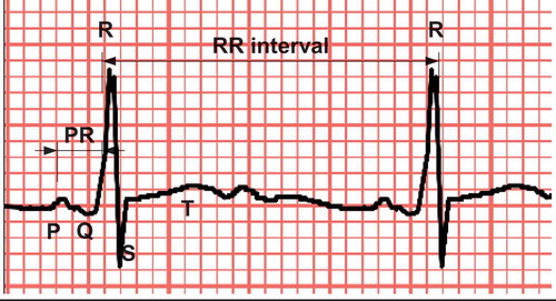
Each phase of the ECG signal has limited amplitude and a limited duration as stated in Table 1 (Jambukia, Dabhi, and Prajapati 2015). Deviation from these values can indicate damages to the hearts conducting system or to its cells. Especially morphology and rate changes can indicate a serious cardiac arrhythmia such as ventricular tachycardia or ventricular fibrillation.

Table 1. Selected ECG physiologic features.

Phase	Description	Amplitude/duration
P	The first upwards wave of the ECG	<80 mS
RR	The time interval between to RR peaks	0.6–1.2 S
PR	The time between the P and the R wave	120–200 ms
QRS	Time between Q and S beats	80–120 ms
ST	Time between S and T beats	320 ms

The challenges in monitoring these signals are that morphology and rate changes can be imposed in the form of noise, power-line interference, baseline drift, muscle contraction, and motional artifacts.

VEB or PVC is a group of arrhythmia beats that is triggered from an abnormal electric activity in the ventricles where the signals do not come from the correct electric sources, i.e. the sino atrial node, the atrioventricular node, and the purkinje fibers. Because the PVC does occur without being triggered from the sino atrial node, it is not preceded by a P beat, and it has a wider QRS complex. On an ECG plot, this can be seen as very irregular shapes named multiform. Because the shapes are multiform the morphology of the PVC beats is different from one person to another which makes these very hard to detect in a machine learning setting without using individual supervised learning. However, supervised learning is challenging with respect to getting enough annotated data.

Related Works

Most of the literature which deals with small training sets uses dimensionality reduction techniques like PCA and SVD. However, a problem with this concept is low accuracy for small training set sizes (Raudys et al. 2015). Similar techniques are feature selection and feature extraction, which are very alike to dimensionality reduction techniques (Louis et al. 2017).

A classifier, which is based on a limited amount of training data, is provided by Louis et al. They assumed that the ECG signals are multivariate Gaussian distributions in a generative model, which was used to generate training samples. However, with small sample size, they had instability problems, which were solved by adding parallel classifiers that were trained with more data. It is noted that they used a proprietary database (Toronto database) for validating the scores (Louis et al. 2017). Andreao et al. have used the Hidden Markov Model (HMM) to detect QRS complexes in a selected set from the MIT BIH database. They obtain a beat detector performance where the sensitivity and the positive predicted value (PPV) were above 99%. However, the PVC scores are 87% for sensitivity and 86% for PPV. This difference between QRS and PVC scores clearly supports the facts that high PVC scores are hard to get. Jung et al. used a wavelet-base statistical approach to detect PVC beats, and they achieved a sensitivity of 98%, a specificity of 87%, and a PPV of 85%. However, this approach uses a control variable (α), which needs to be tuned to balance the true positive score against the false positive score, i.e. some amount annotated data are needed (Jung og Heeyoung 2017). Other researchers have looked into the use of Artificial Neural Networks (ANN) to classify arrhythmias. Minami et al. used Fourier transformation and ANN to extract features (Minami, Nakajima og Toyoshima 1999). A low-complexity system has been proposed by Chang et al. which use simple features to classify ECG signals. The scores for this system are above 98% for both sensitivity and specificity; however, the PVC scores are not available in the presented results (Chang et al. 2017). Regarding QRS detection Andrysiak et al. used a sparse ECG signal representation based on dictionaries, and they used neural networks to detect these (Andrysiak 2016). They achieved sensitivity scores beyond 98% in detecting QRS complexes from the MIT-BIH database (MIT 2018). This number is comparable to the QRS detector from Pan et al. which has been used in this work (Pan og Tompkins 1985). Hence, it would be possible to use this detector to find the QRS complexes in future works.

The Arrhythmia Detection Model

To classify ECG signals some steps are required: ECG filtering to remove noise and artifacts; dividing the heartbeat into segments; feature extraction; and feature classification. Regarding ECG filtering most authors’ use simple finite impulse response filters (FIR) because they are stable, they provide linear phase, and they are simple to implement (Chazal, O’Dwyer og Reilly 2004; Yeh, Wang, and Chiou 2009; Luz et al. 2016; Lynn 1979). However, other approaches such as wavelet transform (Saysdi og Shamsollahi 2007) and non-linear filters have been used (de Lannoy et al. 2014). The heart beat signal segmentation step divides the signal into segments, which is processed and used as features in the classification step (Pan and Tompkins 1985; Oster et al. 2015; Hejazi1, et al. 2015; Jambukia, Dabhi, and Prajapati 2015; Murphy 2012).

The previous discussed four steps have been used to design the PVC classifier used in his work. First, the signal is filtered by a FIR filter that removes noise; second, the filtered signal is processed by a QRS detector which indicates the position of the beats in the signal stream. In this work, the QRS detector described by Pan et al. (Pan and Tompkins 1985) is used because it scores more than 99% in specificity and sensitivity (Jambukia, Dabhi, and Prajapati 2015). Third, the ECG signal and the beat positions are processed by the feature extraction step where five features are used in this work. It is noted that increasing the amount of features often increase the classification scores, given that the features are uncorrelated and that the classifier variance is within reasonable limits. Nevertheless, as previously discussed the PVC classifier designed in this work uses a very limited amount of annotated training data, which means that the number of features must be kept low to balance the model complexity (bias-variance) and to overcome the “curse of dimensionality” paradigm (Theodoridis and Koutroumbas 2008). Hence, five features have been selected where three of these (feature 1, 4, and 5, Table 2) have been selected because they provide high scores in most PVC-related classifiers (Jambukia, Dabhi, and Prajapati 2015). The two last features have been developed with focus on classifying PVC patterns only (features 2 and 3, Table 2). These features are inspired from the facts that: physiologically there is no premature beat (P beat) before a PVC beat, they are robust in noisy environments, and they are uncorrelated to the other features. The final step is selecting a classifier for this work. Because of the very limited amount of annotated training data used for supervised learning in this work a multivariate probabilistic classifier has been chosen. This classifier offers accessibility to classifier-uncertainty and it offers robustness to dichotomous variables (Herault og Grandvalet 2007; William 1980). It is noted that the “no free lunch” theorem states that there is no one model that works best for every problem, which means that other classifier types could provide acceptable results, given the limited amount of training data (Wolpert og Macready 1997). The used multivariate probabilistic classifier is a hybrid between a regularized Quadratic Discriminant Analysis (QDA) classifier and a regularized Linear Discriminant Analysis (LDA) classifier. This hybrid mix of the well know QDA and LDA classifiers is needed to obtain the benefits from the off diagonal covariance elements as well as the benefits that the principal diagonal is stable (it prevents the covariance matrix from becoming singular). This classifier is a powerful choice which uses a linear combination of features to split classes with the best performance. In addition, it is widely applied in similar applications such as speech recognition, image retrieval, and pattern recognition (Yeh, Wang, and Chiou 2009).

Table 2. Selected features.

Feature no.	Feature symbol	Feature description	Units
1	m_PQ	Find maximal signal value in the PQ interval	Amplitude
2	a_PQ	Calculate the area between the signal in the PQ interval and zero.	Amplitude multiplied with time
3	ms_PQ	Maximal slope in the PQ interval	Samples/time
4	i_RR	Time between two consecutive R beats	Samples
5	i_PR	Time between the P beat and the R beat	Samples

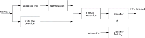
The developed feature extraction model is shown in Figure 2. Leftmost the raw ECG-signal enters the bandpass-filter and the ECG beat detection blocks. After being processed in the bandpass-filter it is normalized and fed to the feature extraction block. Similarly, the signal output from the ECG beat detection block is fed to the feature extraction block. This block extracts characteristic features which describe the morphology of the ECG signal and passes this to the classifier block. The classifier block builds a statistical model from the incoming data in its training phase and uses this model to classify in its classification phase.

Figure 2. The simulation model.

The bandpass-filter limits the ECG signal bandwidth to reduce the influence of power-line interference, baseline drift, muscle contraction, and motional artifacts. Details of the filter design are given below (Figure 3).

Figure 3. Bandpass- filter. The left plot is the roots and zeros (X-axis is the real part, Y-axis is the imaginary part). The right plot is the filter attenuation in DB as a function of input frequency.

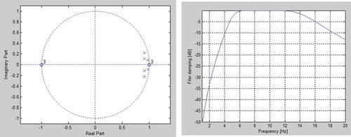
The deployed filter is a 3ʹ order Butterworth band-pass filter which cuts below 5 Hz and above 15 Hz (Figure 3). The position of the three zeros at DC and the three complex poles inside the pass-band provides a high damping below the lower limit of the filter. This is necessary to reduce the relatively high amplitude often found in baseline drift, in muscle contraction, and in motional artifacts. Above the pass-band three zeros are located at half the sampling frequency to provide filter attenuation and to reduce the impact from power-line interferences. The filter is deployed by convolving the filter coefficients with the samples.

The normalization block finds the largest amplitude in the filtered signal and normalizes the signal with respect to this Equation (1).

(1) $\begin{array}{c}j=\underset{n}{argmax}({S^{\prime }}_n)wheren\in \left\{1,2,...,N\right\}\\ S_n=\frac{{S^{\prime }}_n}{S_j}\end{array}$(1)

Where Sn is the incoming sampled ECG signal and S_j is the value of the largest sample.

The ECG beat detection block is a strait forward implementation of the Pan-Tompkins algorithm. This algorithm is known for being one of the best for detecting beats with sensitivity and specificity scores higher than 99% (Pan and Tompkins 1985). In addition, it is computationally efficient and it includes noise removal steps (Jambukia, Dabhi, and Prajapati 2015).

The feature extraction block processes the characteristics of the ECG signal, i.e. it extracts the location, duration, amplitude, and morphology features. This block is triggered by the ECG beat detection block. As discussed five features have been derived and developed in this work (Table 1). These are based on the fact that: PVC beats are not triggered by the sino-atrial-node, which means that P beats are not generated; the distance between the R beats will be different compared to the distances when a normal sinus rhythm is present; and the distance from the P beat candidate to the following R beat will be different too.

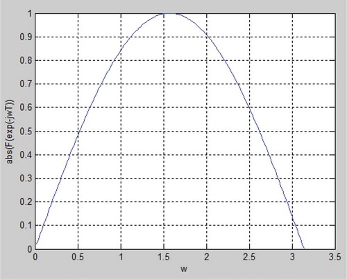
The first feature m_PQ works directly on the filtered and normalized input signal (Table 2). The first step is to shape a time window in form of samples that represents the time period where a P beat would be expected. As stated in Table 1, the minimum time for the PR distance is 120 mS and the maximum distance is 200 mS which can be recalculated into samples with a lower limit of 72 samples and a higher limit of 42 samples. To find the maximum of the signal in this sample window, the derivative of the signal is calculated by using a five-point derivative approximation with the transfer function F(z). By substituting z with exp(-jωT) the absolute transfer function can be plotted in a normalized sample space (Figure 4). It is noted that the transfer function behaves as a derivate as long as the frequency is blow approximately ω = π/4, (approximately 90 Hz) which is below the upper bandpass-filter limit.

Figure 4. The derivative of function (F(Z) and the absolute transfer function for F(Z).

After taking the derivative of the signal its maximum can be located where the slope is low and the signal value is high Equation (2). In this equation C is a constant, R(n) is the position of the R beat number n, Sll is the low limit and Shl is the high limit in samples.

(2) $\begin{array}{rl}& Q\subseteq S\because Q(n,m)=S(R(n)-Sll+1+m)wherem\in \{0,1,...,Sll-Shl\}\\ & Q_{\mathrm{\Delta }}(n,l-2)=\frac{1}{8T}(-Q(l-2)-2Q(l-1)+2Q(l+1)+Q(l+2))\\ & wherel\in \{2,3,...,Sll-Shl-2\}\\ & m\mathrm{\_}PQ(n)=\underset{k\in K}{argmin}(\left|Q_{\mathrm{\Delta }}(n,k)\right|-C\cdot Q(n,k))whereK\in \{0,1,...,Sll-Shl-4\}\end{array}$(2)

A plot of this feature for two ECG signals (MIT-BIH database sets 119 and 217) are provided in The a_PO feature calculates an area approximation (in sample space) between the PQ interval and the zero level for the R beat number n Equation (3).

(3) $a\mathrm{\_}PQ(n)=\frac{1}{Sll-Shl-3}\sum _{m=0}^{Sll-Shl-4}Q(n,m)$(3)

By plotting this feature, it is noted that the areas are very different for N beats compared to the V beats (MIT-BIH database sets 119 and 217, Figures 5 and 7). This plot indicates that the variance and the mean values for the multivariate Gaussian distributions are different, which increases the probability for correct classification.

Figure 5. A histogram of the five features when the MIT-BIH set 217 is processed.

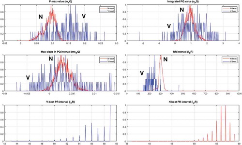
Figure 6. ECG set 217: A time/amplitude plot and the reduction in mutual information when one of the features (5) is left out.

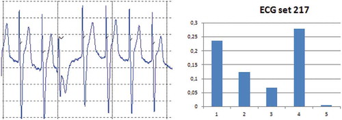
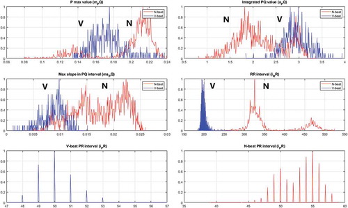
Figure 7. A histogram of the five features when the MIT-BIH set 119 is processed.

The ms_PQ feature expresses the maximum slope of the signal in the PQ interval Equation (4).

(4) $ms\mathrm{\_}PQ(n)=\underset{m}{max}(Q_{\mathrm{\Delta }}(n,m))wherem\in \left\{0,1,...,Sll-Shl-4\right\}$(4)

A plot of this feature is provided in Figures 5 and 7 for the MIT-BIH database sets 119 and 217. Similarly to the a_PO feature the variance and mean values can be separated by a classifier.

The i_RR feature is found by counting the number of samples there are between two adjacent R beats. A similar process is used for the i_PQ beats. A plot of these features is provided in Figures 5 and 7 for the MIT-BIH database sets 119 and 217.

After being processed in the feature extraction block, the generated feature-vector is fed to the classification block (Figure 2). This block implements a regularized quadratic/linear discriminant analysis classifier named Regularized Discriminant Analysis (RDA), which assigns the feature vector to one (and only one) of K classes. Formally, the feature-vector is assumed to be a member of one class only and assignments to any other classes is considered a misclassification. Hence, the goal is to design a misclassification risk function R(y = clx,θ) which can then be minimized Equation (5).

(5) $R(\vec{y}=\tilde{c}\left|\vec{x},\vec{\theta })\right.=\frac{\sum _c{\pi }_c(1-\delta (\tilde{c},c))\left|2\pi {\sum _c}^{-\frac{1}{2}}\right|exp\left[-\frac{1}{2}{(\vec{x}-{\vec{\mu }}_c)}^T\sum _c^{-1}(\vec{x}-{\vec{\mu }}_c)\right]}{{\sum }_{c^{\prime }}{\pi }_{c^{\prime }}\left|2\pi {\sum _{c^{\prime }}}^{-\frac{1}{2}}\right|exp\left[-\frac{1}{2}{(\vec{x}-{\vec{\mu }}_{c^{\prime }})}^T\sum _{c^{\prime }}^{-1}(\vec{x}-{\vec{\mu }}_{c^{\prime }})\right]}$(5)

It is assumed that the distribution for the true ECG signals can be approximated by Gaussian distributions (Louis et al. 2017). The risk function uses the dirac-delta function (δ(p,q)), the unconditional prior (πi), the multivariate mean vector (μi), and the multivariate covariance matrix (Σi). Minimizing the risk function Equation (6) leads to the optimal classification rule Copt.

(6) $\begin{array}{rl}& C_{opt}(\vec{x},\vec{\theta })=\underset{\tilde{c}}{argmin}(R(\vec{y}=\tilde{c}\left|\vec{x},\vec{\theta })\right.\\ & =\underset{\mathrm{\forall }\tilde{c}\in C}{argmax}\frac{{\pi }_{\tilde{c}}\left|2\pi {\sum _{{ }_{\tilde{c}}}}^{-\frac{1}{2}}\right|exp\left[-\frac{1}{2}{(\vec{x}-{\vec{\mu }}_{{ }_{\tilde{c}}})}^T\sum _{{ }_{\tilde{c}}}^{-1}(\vec{x}-{\vec{\mu }}_{{ }_{\tilde{c}}})\right]}{\sum _{\mathrm{\forall }c\in C\wedge .c\ne \tilde{c}}{\pi }_c\left|2\pi {\sum _c}^{-\frac{1}{2}}\right|exp\left[-\frac{1}{2}{(\vec{x}-{\vec{\mu }}_c)}^T\sum _c^{-1}(\vec{x}-{\vec{\mu }}_c)\right]}\end{array}$(6)

The optimum class Copt is found when the largest estimated class in the set C is positioned in the numerator of Equation (6), which means that it is sufficient to maximize this Equation (7). This maximization is easily performed by using the Negative Log Likelihood (NLL) (Murphy 2012) where minimizing the NLL is equivalent to maximizing the log likelihood.

(7) $\begin{array}{rl}& C_{opt}(\vec{x},\vec{\theta })=\underset{\mathrm{\forall }\tilde{c}\in C}{argmin}NLL(\vec{x},\vec{\theta })\\ & =\underset{\mathrm{\forall }\tilde{c}\in C}{argmin}((\vec{x}-{\vec{\mu }}_{{ }_{\tilde{c}}}{)}^T\sum _{{ }_{\tilde{c}}}^{-1}(\vec{x}-{\vec{\mu }}_{{ }_{\tilde{c}}})+ln\left(\left|\sum _{{ }_{\tilde{c}}}\right|\right)-2ln({\pi }_{\tilde{c}}))\end{array}$(7)

The optimization equation Equation (7) consists of two parts. The first part is the discriminant function which is all the terms except the last one and the second part is the first term which is the well known Mahalonobis distance (Murphy 2012) between the multivariate feature vector x and a multivariate class mean μ.

The training of the classifier is performed by using multivariate mean μ and multivariate variance Σ ML-estimators on the training data sets Equation (8) where it is assumed that the samples are i.i.d and xi = N(μ,Σ).

(8) $\begin{array}{rl}& \hat{\mu }=\frac{1}{N}\sum _{i=0}^{N-1}{\vec{x}}_i\\ & \sum ^{ˆ}=\frac{1}{N}\sum _{i=0}^{N-1}({\vec{x}}_i-\hat{\mu })({\vec{x}}_i-\hat{\mu }{)}^T\end{array}$(8)

Where the feature vector x_i is constructed by assigning the features one by one to each of the five positions in the vector. The variable N is the number of training sets used in the k-fold cross validation.

This classifier approaches a QDA classifier when individual covariance matrixes are used for each class, and it approaches a LDA classifier when the covariance matrixes for the classes are equal. Especially the covariance matrix is the main challenges in using discriminant analysis with a sparse training dataset, i.e. the size of the dataset is close to the dimensionality of the feature vector. This challenge can be explored by decompose the covariance matrix into its eigenvectors (V) and eigenvalues (D), which can then be used in the discriminant function Equation (9).

(9) $\begin{array}{rl}& dF=(\vec{x}-\vec{\mu }{)}^T(VD{V}^T{)}^{-1}(\vec{x}-\vec{\mu })+ln(\left|VD{V}^T\right|)\\ & =tr(\xi {\xi }^T{D}^{-1})+ln(\left|D\right|)where:\xi =(\vec{x}-\vec{\mu }{)}^{T}V\end{array}$(9)

It is observed Equation (9) that the discriminant function (dF) is heavily weighted by small eigenvalues and the direction of the eigenvectors. Unfortunately, estimators for covariance values are biased so large eigenvalues are biased toward higher values and small eigenvalues are biased toward lower values (Friedman 1988). Many approaches have been tried to remove this distortion from the eigenvalues and to make the covariance matrix nonsingular (Louis et al. 2017; Murphy 2012). Especially in the context with small sample size settings a promising approach is deploying a regularization method that decreases the variance and regulate the covariance principal diagonal. This approach is deployed by using a pooled covariance where a weighted amount of the covariance matrix for the N beats is pooled with the covariance of the V beats. Added to this is a weighted part of the principal diagonal of the pooled covariance matrix itself Equation (10).

(10) ${\hat{\mathrm{\Sigma }}}_n(\lambda ,\gamma )=(1-\gamma )(\lambda {\mathrm{\Sigma }}_v+(1-\lambda ){\mathrm{\Sigma }}_n)+\gamma (tr(\lambda {\mathrm{\Sigma }}_v+(1-\lambda ){\mathrm{\Sigma }}_n)I)$(10)

Where Σ_n and Σ_v are the covariance matrixes for N beats and V beats, respectively. The λ and γ values control the degree of regularization.

The performance of the PVC classifier has been found by comparing classifications in relation to the provided annotations (i.e. the “ground truth”). This comparison has been based on counting (i.e. TP, TN, FP, and FN) as suggested by Jager et al. (Jager et al. 1991). By using this concept, a measure of accuracy, specificity, sensitivity, positive predicted value PPV and negative predicted value NPP can be calculated Equation (11).

(11) $\begin{array}{c}Accuracy=\frac{TN+TP}{TN+TP+FN+FP}Specificity=\frac{TN}{TN+FP}Sensitivity=\frac{TP}{TP+FN}\\ PPV=\frac{TP}{TP+FP}NPV=\frac{TN}{TN+FN}\end{array}$(11)

Model Simulations and Elaborations

The model discussed in the previous section (Figure 2) has been used to classify N beats and V beats in the ECG sets from the MIT-BIH database (MIT 2018). This has been done by using 5-fold validation with 15N and 15V beat samples which have been selected randomly from a full ECG set in the MIT BIH database. It is noted that the selected training samples are excluded from the test sets.

To explore the performance of the PVC classifier with a very sparse amount of annotated training data 10 ECG sets have been selected (Table 3). These series have been selected randomly from the complete sets in the MIT BIH database with the only restriction that there is more than 100 PVC beats in a selected set. This restriction is necessary for ensuring that it is possible to select the training data for the V beats randomly in a k-fold process. To set these scorings into a context, they are compared to results provided by other researchers.

Table 3. PVC classifier scorings on 10 ECG sets from the mit-bih database.

MIT BIH ECG set	Specificity [%]	Sensitivity [%]	Accuracy [%]	PPV [%]	NPV [%]	Total number of beats	PVS beats
106	99	100	100	100	100	2027	520
116	99	100	100	97	100	2412	109
119	99	100	100	100	100	1987	444
200	95	96	96	93	97	1775	826
201	94	98	98	89	99	1802	198
214	97	100	99	98	100	2006	256
217	96	98	98	80	100	2208	162
221	97	99	99	95	99	2031	396
223	90	96	95	84	98	2605	473
233	93	99	98	98	97	2249	831

Regarding the regularization parameters λ is set to 0.1 and γ is set to 0.2 by using a trial and error approach, i.e. more research is needed to clarify the settings of these parameters in the context of classifying a nonlinear ECG signal.

It is observed (Table 3) that the results from the PVC classifier on the ECG sets in general score above 90% for most sets, which is acceptable taken into consideration that the training set consists of 30 annotated beats only. It is noted that two ECG sets stands out (119 and 217). ECG set 119 scores beyond 99% in all measures, whereas ECG set 217 scores lower with a score of 80 on its PPV measure. To explore these deviations in relation to the features a histogram for each of them are plotted together with their time/amplitude and their Reduction in Features Mutual Information (RFMI) (Figures 5–8). The plotted histograms contain the five features where the curve is the normalized number of N/V beats (y-axis) together with its relative feature values (x-axis). Regarding the RFMI plot it expresses the reduction in mutual information between the classifier output and each individual feature. The “backwards principle” has been used, i.e. one feature is removed at a time given that all other features are present (it is noted that these will not sum to 100% because the percentage is relative to the RMFI when no features are removed). It has been assumed that the features are uncorrelated (Wang og Hu 2009). The principle and equations for calculating the RFMI as a function of the two score metrics can be found in Wang et al (Wang and Bao-Gang 2009).

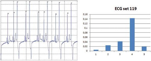
Figure 8. ECG set 119: A time/amplitude plot and the reduction in mutual information when one of the features (5) is left out.

For ECG set 217 its histogram (Figure 5) and RFMI (Figure 6) have been plotted. It is noted that the low PPV score is caused by an increase in the FP count, i.e. some N beats have been classified as V beats. One reason for this can be found by examining the time/amplitude where it is observed that this ECG set is from a patient with a pacemaker that paces in the ventricles, i.e. the systoles are initiated by this. However, the designed features detect that the P beat is absent in the PVC patterns, but in this paced rhythm there is no P beat because the pacing takes place directly in the ventricles, so it seems as the features behaves as expected. From the FMRI plot it is observed that removing one of the features 1 to 4 will reduce the FMRI with a considerable amount. It turns out that feature 5 only reduces the FMRI with less than 1%, i.e. the contribution from this feature is limited in this ECG set. Similarly, the reduction in the PPV score can be seen from the histogram plot where it is observed that the variance of the V beats and the N beats are close to being similar. In addition, it is observed that the mean values of these distributions are close to coincide. Thus, the overlapping variances and mean values cause some N beats to be classified as V beats, i.e. it increases the FP measure.

As discussed ECG set 119 performs very well. The reasons for this can be found by performing a similar analysis as for ECG set 217, i.e. its histogram (Figure 7), time/amplitude, and RFMI (Figure 8) have been plotted. From the RFMI score it is noted that most of the features contribute to the high scores. Actually the new developed PVC features (feature 2 and 3) perform well with a stable contribution and with a limited variance. Additional insight can be found by looking into the histogram for these features where it is noted that the distributions of the beats are more separable compared to the distributions for ECG set 217.

In general, it is noted that the contribution of each feature depends on the selected beat set, which indicates that the ECG signals have a large spreading on their morphology and signal composition, i.e. they need to be handled by dissimilar robust features.

The ECG set scores as a function training set size needs some clarification. As already discussed, the size of the training data must exceed the number of features considerably (dimensionality of the feature vector) to prevent the covariance matrix from becoming singular. However, the regularization used in this work enables the size of the training data to come very close to the number of features. This means that it is possible to perform the classification with a very small training set size. To substantiate this important result the same ECG set that was used with the 15N and 15V beats (Figure 9) have been used for a 10N and 10V (Figure 10) beats set and for a 5N and 5V beats set (Figure 11).

Figure 9. Scores (Y-axis) for the randomly selected ECG sets (X-axis) with 15N and 15V beats in the training set.

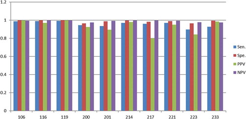
Figure 10. Scores (Y-axis) for the randomly selected ECG sets (X-axis) with 10N and 10V beats in the training set.

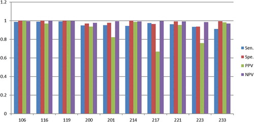
Figure 11. Scores (Y-axis) for the randomly selected ECG sets (X-axis) with 5N and 5V beats in the training set.

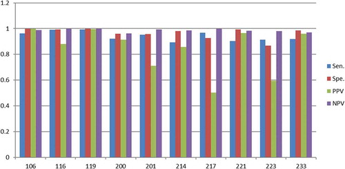
As discussed, the scores for the 15N and 15V beats (Figure 9) are close to 90% for most ECG sets (except PPV score for 217 and 223). By reducing the training set size to 10N and 10V beats it turns out that the scores drop a few percentages except for the PPV scores in set 217 and set 223, which drops considerably more (Figure 10). The same tendency is found when the training set size drops to 5N and 5V beats (Figure 11). At this very low training set size the scores for most of the sets fluctuates considerably, which indicates that few eigenvectors and eigenvalues in the covariance matrix dominates and they vary considerably, i.e. they introduces the instability.

To substantiate these importance results they are compared with scores from other researchers. Luz et al. provides a comparison from five authors which are averaged to one score in this work (Luz et al. 2016). Their scores provide a specificity of approximately 85% and a PPV of approximately 89% (Table 9). Similarly, Christov et al. compared four authors (Christov, Jekova og Bortolan 2005), which when averaged provide a specificity of 98% and a sensitivity of 96%. Oster et al. compared six authors which when averaged provide a specificity of 92% and a PPV of 92% (Oster et al. 2015). It is noted that these authors uses the full dataset in different k-fold based training and testing procedures – not only 15N and 15V beats. The multivariate Gaussian model presented by Louis et al. is able to handle 30 beats training data; however, they used the proprietary Toronto database for validating the performance of their system. This means that their result is not directly comparable with the results from the MIT-BIH database; however, for the sake of completeness their error percentage (7%) is added to Table 4 (Louis et al. 2017). In addition, a comparison presented by Louis et al. (Table 5 in their paper) is averaged and added to Table 4.

Table 4. The PVC classifier scores compared with scores from similar works.

No.	Author	Sen. [%]	Spe. [%]	PPV [%]	NPV [%]
1	This work (15N/15V)	96	99	93	99
2	Luz et al. (average over 5 authors) (Luz et al. 2016)	Not provided	85	89	Not provided
3	Christov et al. (average over 4 authors) (Christov, Jekova, and Bortolan 2005)	96	98	Not provided	Not provided
4	Oster et al. (average over 6 authors) (Oster et al. 2015)	Not provided	92	92	Not provided
5	Louis et al. (Louis et al. 2017)	Error percentage of 7% on the proprietary Toronto database
6	Louis et al., Table 5, (average over 5 authors) (Louis et al. 2017)	Error percentage of 13% on the proprietary Toronto database

From Table 4 it is noted that the PVC classifier performs comparable to similar works (even though author number 2 to 4 uses larger training data sets in a k-fold manner).

Conclusion

In this work, a novel PVC classifier has been presented, which provides very good results in relation to similar classifiers where it is noted that comparable classifiers uses much more data for training in form of a k-fold spilt of the data. In contrast, the developed PVC classifier only uses supervised annotated data in form of 15N beats and 15V beats to obtain an average performance of more than 96% in accuracy, specificity, and sensitivity and more than 93% in the PPV and NPV scores. These non-trivial results indicate big potentials in designing robust PVC classifiers which can be trained with only 30 classified beats (classified by an expert). It is noted that a training set size of 30 beats is the upper limit to obtain the discussed performance which means that many beat patterns can be trained with fewer annotated beats to obtain similar performance; however, some PVC signals are sensitive to less training data which means that lower scores must be expected in these cases.

The novelty of the presented PVC classifier is rooted in the use of solid and robust feature designs in combination with an advanced regularization method. The five features consist of three selected features in combination with two novel features designed for detecting PVC beats only. These features work well for most of the beat sequences in the MIT-BIH database; however, set 119 and 217 stand out. Set 119 is a sinus rhythm with some embedded PVC extra systoles. By analyzing the behavior of the features on set 119 it has been found that they provide clear clusters, and their mutual information show that all features contribute, which means that this rhythm gets high scores. In contrast, sequence 217 is a paced rhythm where a pacemaker initiates the systoles. These systoles have very similar characteristics and morphologies to PVC patterns why they are very difficult to classify. Nevertheless, it has been found that all features contribute so a linear combination of these makes this rhythm detectable. An improvement of this work could be to add an extra feature which detects the pacemaker beats, which most likely would increase the scores for sequence 217.

Finally, the PVC classifier has been tested (5-fold) with a reduced amount of training data where the set sizes is reduced to 20 (10N and 10V) and 10 (5N and 5V) beats respectively. The average performance of the PVC classifier only drops a few percents on these very sparse training sets; however, a tendency to classifier instability is found with the smallest amount of training data (5N and 5V), why relaying on this very limited training data size is not recommended.

References

- Andrysiak, T. 2016. Machine learning techniques applied to data analysis and anomaly detection in ECG signals. Applied Artificial Intelligence 30:610–34. doi:10.1080/08839514.2016.1193720.
- Chang, R., H. Chen, C. Lin, and K. Lin. 2017. Design of a low-complexity real-time Arrhythmia detection system. Journal of Signal Processing Systems90(1): 145–156.
- Chazal, P., M. O’Dwyer, and R. Reilly. 2004. Automatic classification of heartbeats using ECG morphology and heartbeat interval features. IEEE Transaction on Biomedical Engineering51(7): 1196–1206.
- Christov, I., I. Jekova, and G. Bortolan. 2005. Premature ventricular contraction classification by the Kth nearest-neighbours rule. Physiological Measurement 26:123–30. doi:10.1088/0967-3334/26/1/011.
- de Lannoy, G., D. Franc¸Ois, J. Delbeke, and M. Verleysen. 2014. Weighted conditional random fields for supervised interpatient heartbeat classification . IEEE Transaction on Biomedicine Engineering59(1): 241–247.
- Friedman, J. 1988. Regularized discriminant analysis. Journal of the American Statistical Association84(405): 165–175.
- Hejazi1, M., S. A. R. Al-Haddad, Y. P. Singh, S. J. Hashim, and A. F. A. Aziz. 2015. Multiclass support vector machines for classification of ECG data with missing values. Applied Artificial Intelligence 29:660–74. doi:10.1080/08839514.2015.1051887.
- Herault, R., and Y. Grandvalet. “Sparse probabilistic classifiers.” Proceedings of the 24 th International Conferenceon Machine Learning.Corvalis, OR. 2007.
- Jager, F., G. Moody, A. Taddei, and R. Mark. 1991. Performance measures for algorithms to detect transient ischemic ST segment changes. IEEE Computer Society Press Advertisement1991, 369–372.
- Jambukia, S., V. Dabhi, and H. Prajapati. “Classification of ECG signals using machine learning techniques: A survey.” International Conference on Advances in Computer Engineering and Applications (ICACEA). IMS Engineering College, Ghaziabad, India. 2015.
- Jung, Y., and K. Heeyoung. 2017. Detection of PVC by using a wavelet-based statistical ECG monitoring procedure. Biomedical Signal Processing and Control 36:176–82. doi:10.1016/j.bspc.2017.03.023.
- Louis, W., S. Abdulnour, S. Haghighi, and D. Hatzinakos. 2017. On biometric systems: Electrocardiogram Gaussianity and data synthesis. EURASIP Journal on Bioinformatics and Systems Biology 2017. doi: 10.1186/s13637-017-0056-2.
- Luz, E., W. Schwartz, G. Camara-Chavez, and D. Menotti. 2016. ECG-based heartbeat classification for arrhythmia detection: A survey. Computer Methods and Programs in Biomedicine 127:144–64. doi:10.1016/j.cmpb.2015.12.008.
- Lynn, P. 1979. Recursive digital filters for bioloical signals. Medical & Biological Engineering and Computing9(1): 37–43.
- Minami, K., H. Nakajima, and T. Toyoshima. 1999. Real-time discrimination of ventricular tachyarrhythmia with Fourier transformation neural network. IEEE Transaction Biomedical Engineering 46:179–85. doi:10.1109/10.740880.
- MIT. 2018, April. www.physionet.org.
- Moody, G., and R. Mark. 2001. The impact of the MIT-BIH arrhythmia database. IEEE Engineering in Medicine and Biology Magazine 20:45–50. doi:10.1109/51.932724.
- Murphy, K. P. 2012. Machine learning a probabilistic perspective. Cambridge, Massachusetts: MIT press.
- Oster, J., J. Behar, O. Sayadi, S. Nemati, A. Jhonson, and G. Clifforf. 2015. Semisupervised ECG ventricular beat classification with novelty detection based on switching Kalman filters. IEEE Transactins on Biomedical Engineering 62:2125–34. doi:10.1109/TBME.2015.2402236.
- Pan, J., and W. Tompkins. 1985. A real-time QRS detection algorithm. IEEE Transaction on Biomedicine Engineering. doi:10.1109/TBME.1985.325532.
- Raudys, S., V. Valaitis, Z. Pabarskaite, and G. Biziuleviciene 2015. A price we pay for. http://link.springer.com/chapter/10.1007/978-3-319-16480-9_29.
- Saysdi, O., and M. Shamsollahi. 2007. Multiadaptive bionic wavelet transform: Application to ECG denoising and baseline wandering reduction. Advanced Signal Processing 2007: 1–11.
- Theodoridis, S., and K. Koutroumbas. 2008. Pattern recognition. Burlington, MA: Academic Press.
- Wang, Y., and H. Bao-Gang. 2009. Derivations of normalized mutual information in binary classifications. In Proceedings of the 6th International Conference on Fuzzy Systems and Knowledge Discovery, Vol.1: 155–163.
- William, K. 1980. Discriminant analysis. Thousand Oaks, CA: Sage Publications.
- Wolpert, D., and W. Macready. 1997. No free lunch theorems for optimization. IEEE Transactions on Evolutionary Computation 1:67–82. doi:10.1109/4235.585893.
- Yeh, Y., W. Wang, and C. Chiou. 2009. Cardiac arrhythmia diagnosis method using linear discriminant analysis on ECG signals. Measurement 42:778–89. doi:10.1016/j.measurement.2009.01.004.