Using Genetic Algorithm and ELM Neural Networks for Feature Extraction and Classification of Type 2-Diabetes Mellitus

ABSTRACT

An automated system for early diagnosis of type 2-diabetes mellitus is proposed in this paper, by using the Extreme Learning Machine neural network for classification and the evolutionary genetic algorithms for feature extraction, to be employed on a real data set from Saudi Arabian patients. The dimension of the feature space is reduced by the genetic algorithms and only the effective features are selected. The data is then fed to an Extreme Learning Machine neural network for classification. Diabetes is a major health problem in both industrial and developing countries, and when it appears in pregnancies it may cause many complications, hence its early diagnosis is beneficial for both mother and fetus. Our hybrid algorithm, the GA-ELM algorithm, has produced an optimized diagnosis of type 2-diabetes patients and classified the data set with an accuracy of 97.5% and with six effective features, out of the original eight features given in the dataset. Moreover, comparisons of the GA-ELM method with other available methods were conducted and the results are promising.

Introduction

Diabetes is a lifelong condition that affects the body’s ability to use the energy coming from food in meals. Gestational diabetes Mellitus (GDM) is a form of type 2-diabetes that occurs in women during pregnancy. According to the International Diabetes Federation (IDF), more than 21 million pregnancies were affected by diabetes during the year 2013 (National Diabetes Services Schema (NDSS) 2017). About 12.14% of pregnant women will develop GDM, usually around the 24th to 28th week of the pregnancy. Most women stop having diabetes after the baby is born; however, some women will continue to have high blood glucose levels after delivery. Women with diabetes can have a healthy baby, but there are extra risks during pregnancy to both mom and baby. With careful planning and support from a team of health-care professionals, these risks can be reduced and controlled. Saudi Arabia is among the top 10 countries in the world with the highest occurrence of GDM. A recent report from Riyadh estimated the prevalence of pre-gestational Diabetes Mellitus (Pre-GDM) and (GDM) to be 4.3% and 24.3%, respectively. This reflects high diabetes among pregnant women compared to other populations in the world (Wahabi et al. 2017). In fact, there were 3.4 million cases of diabetes in Saudi Arabia in 2013 (Wahabi et al. 2017). Saudi Arabia is one of the 19 countries of the IDF MENA (Middle East and North Africa) region, where out of the 415 million people having diabetes in the world more than 35.4 million people are in the MENA Region, as seen in Figure 1. Furthermore, by 2040 this number will rise to 72.1 million in that region.

Diabetes is a health challenge which is a highly complex complication and important to be early diagnosed. It is caused by the improper production of insulin in the human body. Insulin is the key parameter responsible to regulate the glucose in the blood. Diabetes can lead to many other risks, including kidney disease, blindness, heart disease and never damage. Diagnosis of Diabetes can be done through routine blood checkup. Diabetes can be controlled by healthy food habits and an appropriate exercise program. Still, there is no permanent cure for diabetes, diagnosis of diabetes needs special care by a physician with a prior diagnosis of the symptoms and deep knowledge of the patient’s history. Moreover, medical tests can be both expensive and tiring to patients; hence, the automation of these tests is preferable. Thus, to make the diagnosis faster and easier, many machine learning techniques are designed for the automatic diabetes diagnosis. Decision support systems in the field of medical diagnosis have increased in recent decades and became a necessity. Design of medical expert systems has created more interest among researchers all over the world. Automated systems use computer-aided diagnosis (CAD) techniques for the prediction of diseases based on certain parameters. Pattern recognition and data mining provide a useful analysis of such medical data. Most common data mining technique for decision-making from real-world data is the classification methods. Usage of data directly could affect the system performance, hence selecting affective features or attributes can have more influence on the performance and the results. Selection of the best features will have more impact on the accuracy of the diagnosis system in prediction (Foroutan and Sklansky 1987), and may save time. There are many researches in the literature done on using computation methods for diabetes diagnosis. Huang and Wang (2006) proposed a general adaptive optimization search methodology and Grid Algorithm combined with Support Vector Machines (SVM) classifier. Another approach by Ren and Bai (2010) have proposed two SVM parameter optimization approaches, GA-SVM and PSO-SVM, and an objective function which is based on the leave-one-out cross-validation, and the SVM parameters are optimized by using GA (Genetic Algorithm) and PSO (particle swarm optimization) respectively. Some other researchers have used automated diagnosis on the Pima Indian diabetes dataset (Aishwarya and Anto 2014) available publicly and they have used methods such as GA-ELM (Aishwarya and Anto 2014) and a combination of several neural networks classifiers in (Temurtas, Yumusak, and Temurtas 2009). Fayssal and Chikh (2013) have designed a diagnosis system for diabetes using Fuzzy classifier and modified Artificial Bee Colony algorithm. Even though the accuracy of this system is low. it has paved the way for further researchers to improve the accuracy. Zhu, Xie, and Zheng (2015) proposed a multiple classifier system from data mining techniques to early detect type 2-diabetes mellitus and have shown good results. Another research paper shows Type 2 diabetes mellitus screening and risk factors using a decision tree, by Habibi, Ahmadi, and Alizadeh (2015).

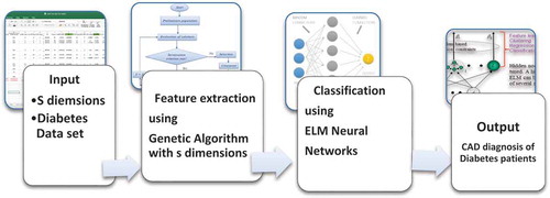
In our research paper, we will present a CAD approach to diagnose diabetes patients from healthy ones based a set of attributes, consisting of a combination between the Extreme Learning Machine (ELM) neural networks and the genetic algorithms (GA). First, a GA attribute selection algorithm is applied for the identification of the effective attributes in the dataset, then the ELM is used for classification, as seen in Figure 2. This paper is organized based on the following sections. Sections II and III describe the background of GA for feature extraction and ELM neural networks for classification, respectively. Section IV describes the GA-ELM method, the Diabetes dataset, and the results. Finally, section V presents the conclusion.

Figure 1. Saudi Arabia, Mena (Middle east and North Africa region) and the world prevalence of diabetes given by Age (Wahabi et al. 2017).

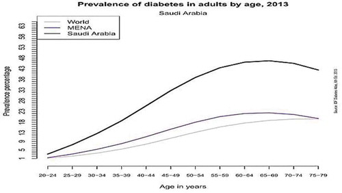
Figure 2. The basic structure of a GA-ELM approach.

Genetic Algorithms for Features Extraction

In pattern recognition, the classification of data is based on the set of selected data features used in the experiment. Therefore, feature selection and extraction are crucial in optimizing performance, and time efficiency, and strongly affect the classifier design. Defining appropriate features often require knowledge by experts in the application area. In practice, there is much noise and redundancy in high dimensional and complex patterns. Therefore, it is sometimes difficult even for experts to determine a minimum or optimum feature set. The “curse of dimensionality” becomes a problem in both statistical pattern recognition (SPR) and artificial neural network (ANN). The selection of appropriate features is an important precursor to most pattern recognition methods (Narendra and Fukunaga 1977; Vafaie and De Jong 1993). A good feature selection mechanism helps to facilitate classification by eliminating noisy or non-representative features that can impede recognition. Even features which provide some useful information can reduce the accuracy of a classifier and become a burden when the amount of training data is limited (Foroutan and Sklansky 1987). Demonstrating the utility of obtaining a minimum-sized set of features that allow a classifier to discern pattern classes well is highly preferred. Feature selection is an important step in designing an automatic medical diagnosis system, because of the large number of data available for real medical cases. There are many approaches that can handle this step in a pattern recognition system. The features derived from the feature extraction step proceed according to their rank and priority to the classifier. The problem of considering the features selection individually is that it ignores the correlation information between the features but they have the advantage of being fast in computation. In contrast. the feature vector selection approaches normally provide better performances at the cost of more computational load. The heuristic search approaches can be employed to use the advantage of feature vector selection strategies and avoid the full search of the feature space. One of these approaches is the genetic algorithms (Punch et al. 1993).

The genetic algorithm method is an iterative procedure that involves a population representing the search space for solutions to the problem, as individuals, each one is represented by a finite string of symbols, called the genome. The basic genetic algorithm proceeds as follows: an initial population of individuals is generated at random or heuristically (Goldberg 1989). In every evolutionary step (generation step), the individuals in the current population are decoded and evaluated according to a fitness function that describes the optimization problem in the search space. To form a new population, individuals are selected according to their fitness (Koza 1992). This ensures that the expected number of times an individual is chosen is approximately proportional to its relative performance in the population. Thus, high-fitness individuals stand a better chance to reproduce and bring new individuals to the population, while low-fitness will not. This process mimics natural selection, and it generates solutions to optimization problems using techniques inspired by natural evolution, such as inheritance, mutation, selection, and crossover (Michalewicz 1996; Mitchell 1996).

Genetic algorithms have been applied to the problem of feature selection by many researchers such as Siedlecki and Sklanski (1989). where they used the genetic algorithm to perform feature selection in combination with a KNN classifier, which is used to evaluate the classification performance of each subset of features selected by the GA. The GA maintains a feature selection vector consisting of a single bit for each feature, with a 1 indicating that the feature participates in KNN classification, and a 0 indicating that it is omitted. The GA searches for a selection vector with a minimal number of 1’s, such that the error rate of the KNN classifier remains below a given threshold. Later work by Punch et al. expanded this approach to use the GA for feature extraction (Punch et al. 1993). Instead of a selection vector consisting of only 0’s and 1’s, the GA manipulates a weight vector, in which a discretized real-valued weight is associated with each feature. A GA-based feature extractor using classification accuracy is utilized as an evaluation criterion. The GA maintains a population of competing for feature transformation matrices. In order to evaluate each matrix in this population, the input patterns are multiplied by the matrix, producing a set of transformed patterns which are then sent to a classifier chosen by the user. The available samples are divided into a training set, used to train the classifier, and a testing set, used to evaluate classification accuracy. The accuracy obtained is then returned to the GA as a measure of the quality of the transformation matrix used to obtain the set of transformed patterns. Using this information, the GA searches for a transformation that minimizes the dimensionality of the transformed patterns while maximizing classification accuracy (Duda, Hart, and Stork 2001).

In the GA feature extraction technique, the choice of features, attributes, or measurements used to represent each pattern presented to the classifier affect the accuracy of the classification function. The attributes used to describe the patterns implicitly define a pattern language. If the language is not expressive enough, it would fail to capture the needed information that is necessary for classification and hence regardless of the learning algorithm used, the accuracy of the classification function learned would be limited by this lack of information (Punch et al. 1993). The feature subset selection problem refers to the task of identifying and selecting a useful subset of attributes to be used to represent patterns from a larger set of often mutually redundant, possibly irrelevant, attributes with different associated measurement costs and/or risks. CAD methods can help in these cases and preform the task of selecting a subset of clinical tests (each with different financial costs, diagnostic values, and risk) to be performed as part of a medical diagnosis task (Alharbi and Tchier 2017; Dalir 2012a, 2012b, 2012c, 2015; Destounis et al. 2004).

Another important aspect in feature extraction by GA is choosing the fitness function, which must measure the accuracy of the classification function realized by the classifier and the cost of performing classification. The accuracy of the classification function can be estimated by calculating the percentage of patterns in a test set that is correctly classified by the neural network used as a classifier in question (Parekh, Yang, and Honavar 1996; Ripley 1996). If S is the number of original features in the problem, then every vector x in the population is of binary form and of length S. Moreover, a “1” indicates that the feature is selected, and a “0” indicates that the feature is not selected. Hence, the proposed fitness function F(x) takes into account two terms: first, the accuracy index, accuracy (x) which is the test of the accuracy of the neural network classifier and the feature subset represented by the x individual. The second term takes into account the cardinality of the subset so as to favor solutions containing a smaller number of features. F (x) can be expressed as

(1) $F\left(\mathrm{X}\right)=\alpha \mathrm{a}\mathrm{c}\mathrm{c}\mathrm{u}\mathrm{r}\mathrm{a}\mathrm{c}\mathrm{y}\left(\mathrm{X}\right)+\pounds \left(\mathrm{S}-\mathrm{s}/\mathrm{S}\right)$(1)

where S is the total number of features available, s is the cardinality of the feature subset represented by x (i.e. the number of bits equal to 1 in the chromosome), and α and £ act as weights to regulate the process’s minimizing priorities. The fitness function guides the GA to search out best feature sets as a multi-objective optimization problem. Running the hybrid computational method yields a small set of “best” classification features which classify the training set more accurately than other sets. By examining those “good” classifiers, one can determine those features which are most useful for classification. Considering a generic application in which a set of samples (say Z) must be classified, and assuming that the samples are represented by means of a set Y of S features, the feature selection problem can be formulated as follows: find the subset X ⊆ Y of s features which optimizes an objective function F. Given a generic subset X ⊆ Y, F (X) measures how well the patterns in Z are discriminated by using the features subset X. Feature subset selection algorithms can be classified into two categories based on whether feature selection is done independently of the learning algorithm used to construct the classifier or not. If feature selection is done independent of the learning algorithm, the technique is said to follow a filter approach. Otherwise, it is said to follow a wrapper approach (Liu and Setiono 1996a). While the filter approach is generally computationally more efficient than the wrapper approach, its major drawback is that an optimal selection of features may not be independent of the inductive and representational biases of the learning algorithm to be used to construct the classier. The wrapper approach, on the other hand, involves the computational overhead of evaluating candidate feature subsets by executing a selected learning algorithm on the data set represented using each feature subset under consideration (Narendra and Fukunaga 1977; Turney 1995). Our proposed approach is a multi-objective feature selection approach wrapped with an ELM neural network classifier.

ELM Neural Networks

Extreme Learning Machine (ELM) is a classic feed-forward neural network with one hidden layer. ELM is an emerging learning algorithm for the generalized single hidden layer feedforward neural networks, of which the hidden node parameters are randomly generated, and the output weights are analytically computed (Huang et al. 2015; Langley 1995). The disadvantage of the feed-forward neural network is its slow process of training, which is due to the fact that the gradient-based approaches, which are used for the training of these networks, are slow. Moreover, all parameters of the network should be tuned iteratively according to a gradient-based approach, which is a very time-consuming process. In the ELM learning approach, the training of a single-layer feed-forward neural network randomly determines the hidden nodes parameters of the network and analytically computes the output weights of the single-layer feed-forward network (Huang, Zhu, and Siew 2004, 2006). Any kind of piecewise nonlinear function can be used for the activation function of the hidden nodes including the RBF, or sigmoid activation functions. Hence, the speed. ELM comes from having just one adjust-able hidden nodes hidden layer and a linear output layer (Huang, Ding, and Zhou 2010; Huang et al. 2012).

The aim of the classification is to find an estimate about a function that relates the samples to their class labels from a set of training samples (Parekh, Yang, and Honavar 1996; Punch et al. 1993). According to this new learning method, if a continuous target function g(X) can be modeled by a single-layer feed-forward neural network with adjustable hidden nodes. The hidden node parameters of such a network can be randomly assigned. To approximate the function g(X), we need the following criterion:

(2) $\underset{N\to \mathrm{\infty }}{\mathrm{l}\mathrm{i}\mathrm{m}}g\left(x\right)-g_N\left(x\right)=\underset{N\to \mathrm{\infty }}{lim}g\left(x\right)-\sum _{j=1}^N{\delta }_{j}K\left(w_j,v_j,x\right)=0$(2)

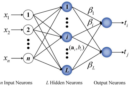
where (w_j,v_j) are randomly generated sequences for the hidden node parameters, the term K(w_j,v_j,x) is the output of the j^th hidden node while the input to the network is x and δ_j indicates the weight of the output layer. The above equation will be satisfied if we choose the parameters δ_j in such a way to minimize the quantity $g\left(x\right)-g_N\left(x\right).$A generalized architecture of the ELM single-layer feed-forward neural network can be seen as Figure 3. In this structure, there are d input nodes equal to the number of features, L hidden nodes. So, the only parameters which must be tuned are those related to output weight vector (Akusok et al. 2015; Ripley 1996). If we consider Z input samples, then we can write the output of the network using the following equation:

$\sum _{j=1}^L{\delta }_{j}K\left(w_j,v_j,x_i\right)=t_i,i=1,\dots ,Z$

where t_i is the target output corresponding to the input of x_i. We can use the matrix form of this equation in the form H δ = T, s.t.

$\mathrm{H}=\left[\begin{array}{c}h\left(x_1\right)\\ ⋮\\ h\left(x_Z\right)\end{array}\right]=\left[\begin{array}{cc}K\left(w_1,v_1,x_1\right)\cdots & K(w_N,v_N,x_{1)}\\ ⋮& ⋮\\ K\left(w_1,v_1,x_Z\right)\dots & K\left(w_N,v_N,x_Z\right)\end{array}\right]$

(3) $\delta =\left[\begin{array}{c}{\delta }_1\\ ⋮\\ {\delta }_L\end{array}\right],andT=\left[\begin{array}{c}{t}_1\\ ⋮\\ t_Z\end{array}\right]$(3)

where T is the target vector, δ is the output weight vector and H is the output matrix of the hidden nodes with respect to the input vectors. The ELM training algorithm goes through the following steps:

1. First, the number of hidden nodes is selected, then the hidden node parameters are determined randomly.

2. Based on the hidden node parameters, the hidden layer output matrix H is computed.

3. The output weight vectors are calculated using the generalized inverse of hidden layer output matrix H by the formula: δ = H⁻¹T where H⁻¹ is the generalized inverse of H.

There are several advantages to the ELM algorithm against traditional training methods like gradient-based algorithms (Akusok et al. 2015; Bai, Kasun, and Huang 2015). The ELM algorithm trains the network in a very fast way and has much fewer parameters to be set. Moreover, the hidden node parameters are determined independently of the training data. Unlike the gradient-based methods, the ELM can work with any non-constant piecewise continuous activation functions that are bounded. Some issues like the local minima, learning rate determination, and overfitting which does not exist with these ELM algorithms. In general, it is a much simpler learning algorithm than other learning algorithms and it has a higher generalization performance compared to other neural network approaches.

Figure 3. ELM neural network structure (Haung et al 2004).

The Genetic – ELM Algorithm

Here we give an overview of the hybrid system proposed for the diagnosis of the diabetes data set. The system consists of a conjunction between a feature selection method which evaluates the feature vectors with the more relevant features for the diagnosis, using a genetic algorithm, and the relatively fast ELM neural network learning algorithm for classification. The selected features given by the GA are fed to the ELM neural network classifier, where the performance of the system is evaluated using the measure of the accuracy of the system and the number of features needed (Bai, Kasun, and Huang 2015; Langley 1995). The classification function realized by ELM is determined by the function computed by the neurons, the connectivity of the network, and the parameters (weights) associated with the connections. A fixed population size of 50 individuals, with the length of each genome set to 8 which is the number of features given in the diabetes data set. Hence, the experiment starts by finding from a population of randomly generated 50 genomes of length 8 bits representing the number of features where the x_i entries are binary, and where a value 1 indicates the features to be kept and a value 0 is for the features to be discarded. The elite candidates (parents) for reproduction are chosen according to their fitness. The crossover between the two chosen parents genome is done at a single point randomly chosen with probability 0.8 to produce the new generation offspring. The selection operator of parent’s genome is set to the stochastic uniform selection method, and the mutation done on the new offspring has probability 0.01. The GA runs throughout the generations to find the best genome in this population representing the feature subset selection. The best genome is the one, which classifies correctly the largest number of the 200 cases (110 Diabetes and 90 Normal cases) given in the dataset, and has the least number of features. Our fitness function F given in Eq.(1) is set to the classification performance, computed as the percentage of cases correctly classified, and the cardinality of the subset features selected, and the minimum of F is found by the GA. After all, 300 generations (repeated 50 times), the genetic algorithm finds the optimum genome; hence, it finds the best feature combination that best classifies the Diabetes dataset. The ELM neural net is trained on this new feature subset training dataset and then tested on the new feature subset testing dataset. The sigmoid activity function is used in the ELM neural net, and the number of hidden neurons are randomly chosen by the net. The algorithm terminates when the maximum number of generations is reached at 300 or when the increase in fitness of the best individual over five successive generations falls below a certain threshold, set at 5 × 10⁻⁶. The Algorithm is as follows:

1. Initialize a random population of individuals (binary of length 8 bits) representing a possible feature subset solution.

2. For 300 generations or while the stopping condition is satisfied:

   1. For each individual x in the population calculate the fitness F(x) by evaluating the data set with the respective features as those represented by the chromosome x using ELM classifier.

   2. Using the stochastic uniform selection method select the most fit individuals for reproduction stage.

   3. Perform crossover on the selected elite individuals, and then mutation on the new offspring’s.

3. After the generations evolve a continuous improvement in the fitness of the generations is observed, and an optimum solution is reached which a subset of features that produce the best classification of the diabetes data set.

The Saudi Type 2- Diabetes Dataset

The Saudi type 2-diabetes Dataset was obtained from King Khalid University Hospital. There are 110 (55%) cases in class (1) and 90 (45%) cases in class (0), Where (1) means a positive test for diabetes and (0) is a negative test for diabetes. Diabetes Attribute information is given below:

1. Number of times pregnant.

2. Glucose tolerance test Fasting Plasma Glucose (FBS).

3. Glucose tolerance test at 1 hours (1H).

4. Glucose tolerance test at 2 hours (2H).

5. Diastolic blood pressure (mm Hg).

6. Hemoglobin A1C HBA1C.

7. Body mass index (weight in kg/height in m).

8. Age (years).

9. Class variable (0 or 1).

The input matrix is a 200 × 8 with the 8 different feature values, and 200 cases. Moreover, we normalized the dataset prior to training, testing, and classification. A linear scaling of features prior to classification allows a classifier to discriminate more finely then feature axes with larger scale factors. The dataset is small and the hospital promised to provide a larger dataset and make it publicly available by next year, for research purposes.

The evolutionary experiments performed fall into the following learning categories, in accordance with the data partitioning into two sets: training set and testing set. The experimental categories are:

1. Training set contains all 200 cases of the database, and the testing is done on the same testing set.

2. Training set contains 75% of the data cases, and the testing set contains the remaining 25% of the cases.

3. Training set contains 50% of the database cases and the testing set contains the remaining 50% of the cases.

4. Randomly assign data points to two sets d0 and d1, so that both sets are equivalent.

In the categories II and III, the choice of training-set cases is done randomly and is performed at the outset of every evolutionary run. MATLAB Genetic Toolbox (Matlab Tool Box Guide) was modified to implement the GA-ELM algorithm, and to generate the graphs of the results. A separate code for the fitness function is called during the procedure according to the fitness function given in Eq.(1). Moreover, every testing of a system is repeated 50 times and the mean and standard deviations are calculated for each experiment. A typical run for 300 generations using all the dataset takes about on average 5.6 min to execute. For each time, the performance of the GA-ELM system in diagnosing of the diabetes dataset was measured and they were averaged over the 50 times repetition of the data dividing (random sub-sampling method). Feature selection based on GA combined with a powerful, fast classifier such as ELM assures a more varied subset of the possible combination of features are evaluated and a better classification result, which leads to better overall performance despite the drawback of having a relatively complicated GA-ELM code.

Results

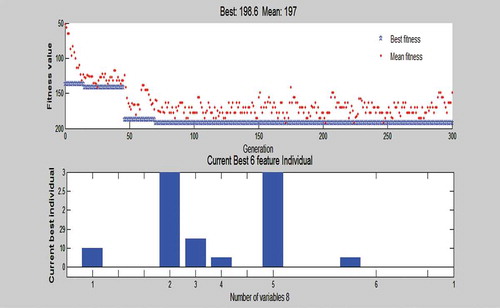
The genetic algorithm generates random sequences of subset combinations and uses the Fitness value to predict the fittest subset of features. We have generated 10 Feature Subset from which one optimal subset can be obtained, which gives the highest fitness value. Table 1, shows the list of all feature subsets generated by the GA. The fitness value of each feature subset depends on the classification accuracy of the system. Classification of these subsets is done by using ELM classifier. We can see the different sets of attributes and its content and performance. Note, the last set with six features shows the best performance with the features: Diastolic BP, HBA1C, Number of Pregnancy, Age, BMI, and GTT (FBS), at an accuracy of 97.5%. Figure 5 shows the performances of these different feature subsets, and we can conclude that the best number of features in the feature subset is 6 with the accuracy of 97.5%. Figure 6 shows the plot of the best fitness value over the generations and the current best individual of the six-feature diagnostic system, taking into account the performance classification rate this system is the top one over all 50 evolutionary runs. The six-attributes selected to best classify the data are Diastolic BP, HBA1C, Number of Pregnancies, Age, BMI, and GTT (FBS). Note, the seventh set with only four attributes has also scored a high accuracy diagnosis rate which means that only these four tests could be conducted for an early diagnosis in case of emergency cases in ER where rapid results are needed.

Table 1. Ten different feature subsets suing GA-ELM and their accuracy.

Set	Number of Attributes	Attributes	Accuracy
1	3	Diastolic BP. Age, BMI	74%
2	3	Diastolic BP, HBA1C, NO. Pregnant	94%
3	3	Age, BMI, HBA1C	92%
4	3	GTT (FBS), Age, BMI	76.3%
5	4	NO. Pregnant, Diastolic BP., Age, BMI	76.2%
6	4	BMI, HBA1C, NO. Pregnant, GTT (1H)	92,8%
7	4	GTT (2H), Diastolic BP, HBA1C, NO. Pregnant	94%
8	5	NO. Pregnant, GTT (1H), Age, BMI, GTT (FBS)	86%
9	5	NO. Pregnant, Diastolic BP, Age, BMI, GTT (FBS)	86%
10	6	Diastolic BP, HBA1C, NO. Pregnant, Age, BMI, GTT (FBS)	97.5%

Figure 4. The comparison of the performances of the four different methods on the same data set.

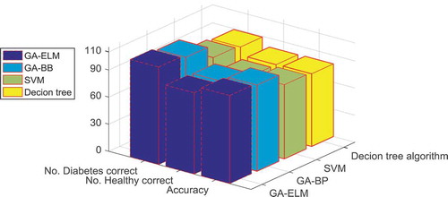
Figure 5. The relationship between the number of features selected in the feature subset and the accuracy of performance.

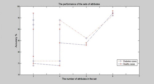
Figure 6. Plots of the best fitness value over the generations and the current best individual of all 8 variables in the 6 feature GA-ELM diagnostic system.

Table 2 presents the average performance obtained by the genetic algorithm with the best six feature subset system over all 50 evolutionary runs, divided according to the four experimental categories. In the first category, we trained the system with all the data and then tested it with the same set of data. In the fourth category, a simple variation of k-fold cross-validation, for each fold, we randomly assign data points to two sets d0 and d1, so that both sets are equal size (this is usually implemented by shuffling the data array and then splitting it in two). We then train on d0 and test on d1, followed by training on d1 and testing on d0. This has the advantage that our training and test sets are both large, and each data point is used for both training and validation on each fold. The performance value denotes the percentage of cases correctly classified and with high confidence. Three such performance values are shown: the performance over the training set; the performance over the test set; and the overall performance on the entire database repeated 50 times, with the mean and standard deviation over the 50 runs in each category.

Table 2. Results divided according to the experimental categories for GA-ELM diagnostic system.

Performance
	Training set	Test set	Overall results for all 50 runs
Training/test 100/100	97.9%	97.9%	Percentage	Mean F(x)	Standard deviation
			98.5%	199.4	1.1
Training/test 75/25	96.30%	96.21%	96.32%	197.4	1.4
Training/test 50/50	96.50%	96.61%	96.32%	198.6	1.4
Training/test d0/d1	96.05%	96.01%	97.5%	198.6	1.3

Comparisons of GA-ELM Results to Other Baseline Methods

In order to analyze the performance of our GA-ELM hybrid approach in classification and feature extraction of GDM dataset, we compare our method with other baseline methods, such as the simple decision tree algorithm, the SVM and the back-propagation neural network approach. For the back-propagation neural network approach, which is a well-known classification method, we use the MATLAB built-in code for Training a neural network called NEWFF, which uses a two-layer feedforward network. The network has a hidden layer of 10 neurons and is trained for up to 50 epochs to an error goal of 0.01, it is then combined with the GA feature extraction code and then applied to the same Saudi type 2-diabetes data set. We also applied the SVM method for classification of the same data set. SVM is a supervised learning method which simultaneously minimizes the empirical classification error and maximizes the geometric margin. SVM is called Maximum Margin Classifiers. SVM is a general algorithm based on guaranteed risk bounds of statistical learning theory, i.e., the so-called structural risk minimization principle. SVM can efficiently perform non-linear classification using what is called the kernel trick, implicitly mapping their inputs into high-dimensional feature spaces. The kernel trick allows constructing the classifier without explicitly knowing the feature space. The Radial Basis Function (RBF) kernel of SVM is used as the classifier, as RBF kernel function can analyze higher-dimensional data. A simple decision tree algorithm is also used on the same data set similar to the procedure done in (Habibi, Ahmadi, and Alizadeh 2015). The technique of decision tree and J48 algorithm, which is the most important algorithm used for developing the decision tree in WEKA (3.6.10 version), was applied to develop the prediction model. J48 is WEKA’s implementation of Quinlan’s C4.5 for building the decision tree Knowledge flow environment, and is one of the WEKA environments for performing the algorithm mentioned. Comparison results of all four methods are given in Table 3. The performance of GA-ELM classifier is compared to GA-BP, SVM, and Decision tree algorithm, with the number of diabetes cases correctly classified, and the number of healthy cases correctly classified for all the available methods recorded. The overall performance of the proposed methods are given in Table 3, in terms of accuracy the GA–ELM system distinguished diabetes subjects with a superior accuracy rate of 97.5%, with only two wrong diagnosis in the diabetes cases and all healthy cases were diagnosed correct, better than the GA-BP method which had wrong diagnosis on both healthy and diabetes cases. Moreover, in terms of speed, the GA-ELM is more efficient since GA-BP takes on average of 10.3 min to execute, with similar code complexity. SVM and the decision tree algorithms have simple code application and consume less time but the results are not very reliable. Hence, as can be seen in Figure 4 the results of the classification of the Saudi diabetes data set using GA-ELM method is best in terms of accuracy compared the other classification techniques. Moreover, feature selection based on GA combined with a powerful classifier such as ELM assures a more varied subset of the possible combination of features are evaluated and better classification results, which leads to better overall performance than simple statistical algorithms or simple classifiers.

Table 3. Comparing overall results for a six feature GA-ELM system in our work with other approaches’ GA-Backpropagation neural network, SVM, and Decision tree algorithm on the same data set.

Research Method	This work GA-ELM	GA-BP	SVM	Decision tree algorithm
Performance	97.5%	95.32%	82%	80.4%
No. of Diabetes correctly classified	108	105	91	89
No. Healthy correctly classified	90	89	80	80

Conclusions

In this study, we introduced a hybrid automated diagnosis system to distinguish the Diabetes pregnant mothers from healthy ones. The proposed method is based on feature selection using the genetic algorithm which discovers those features that are more relevant for the diagnosis of the Diabetes dataset. The selected features are then fed to an ELM neural network classifier to find out the number of successfully distinguish cases in a dataset of subjects with only the specified selected features. Feature selection based on GA performed very well, and since it is done randomly it assures a more varied subset of the possible combination of features are evaluated, which leads to a better performance than simple statistical methods or simple classifiers. The investigation of the results shows that the proposed method is efficient for interpretation of GDM diabetes, and can correctly identify more than 97.5% of the subjects, and with six attributes rather than eight which may save time and money for the patient. Also, the best four attributes subset was found that can be used for rapid diagnosis results. Another advantage to our automated diagnosis is that it could be directly done in the lab computer after the six attributes are determined and the automated diagnosis can be sent with lab results for the physician’s approval.

Additional information

Funding

This research project was supported by a grant from the “Research Centre of the Female Scientific and Medical Colleges”, Deanship of Scientific Research, King Saud University.

References

- Aishwarya, S., and S. Anto. 2014. A medical expert system based on genetic algorithm and extreme learning machine for diabetes disease diagnosis. International Journal of Science, Engineering and Technology Research (IJSETR) 3 (5):75–80.
- Akusok, A., K. Bjork, Y. Miche, and A. Lendasse. 2015. High-performance extreme learning machines: a complete toolbox for big data applications. IEEE Open Access 3. 1011–1025.
- Alharbi, A., and F. Tchier. 2017. Using a genetic-Fuzzy algorithm as a computer aided diagnosis tool on Saudi Arabian breast cancer database. Mathematical Biosciences 286 (2017):39–48. doi:10.1016/j.mbs.2017.02.002.
- Bai, Z., L. L. C. Kasun, and G.-B. Huang. 2015. Generic object recognition with local receptive fields based extreme learning machine. INNS Conference on Big Data, San Francisco, August 8–10. doi:10.1016/j.procs.2015.07.316.
- Dalir, M. R. 2012a. Feature selection using binary particle swarm optimization and support vector machines for medical diagnosis. Biomedizinische Technik/Biomedical Engineering 57 (5):395–402.
- Dalir, M. R. 2012b. A hybrid automatic system for the diagnosis of lung cancer based on genetic algorithm and fuzzy extreme learning machines images. Journal of Medical Systems 36,2,1001–1005. Springer US
- Dalir, M. R. 2012c. Automated diagnosis of Alzheimer disease using the scale-invariant feature transforms in magnetic resonance images. Journal of Medical Systems 36 (2):995–1000. Springer US doi:10.1007/s10916-011-9738-6.
- Dalir, M. R. 2015. Combining extreme learning machines using support vector machines for breast tissue classification. Computer Methods in Biomechanics and Biomedical Engineering 18 (2):185–91. doi:10.1080/10255842.2013.789100.
- Destounis, S. V., P. DiNitto, W. Logan-Young, E. Bonaccio, M. L. Zuley, and K. M. Willison. 2004. Can computer-aided detection with double reading of screening mammograms help decrease the false-negative rate? Initial experience. Radiology 232:578–84. doi:10.1148/radiol.2322030034.
- Duda, R. O., P. E. Hart, and D. G. Stork. 2001. Pattern classification. 2nd ed. New York: Wiley.
- Fayssal, B., and M. A. Chikh. 2013. Design of fuzzy classifer for diabetes disease using modifed artifcial Bee colony algorithm. Computer Methods and Programs in Biomedicine 1:92–103.
- Foroutan, I., and J. Sklansky. 1987. Feature selection for automatic classification of non Gaussian data. IEEE Transactions on Systems, Man and Cybernetics 17:187–98. doi:10.1109/TSMC.1987.4309029.
- Goldberg, D. 1989. Genetic algorithms in search, optimization, and machine learning. New York: Addison-Wesley.
- Habibi, S., M. Ahmadi, and S. Alizadeh. 2015. Type 2 diabetes mellitus screening and risk factors using decision tree: Results of data mining. Global Journal of Health Science 7(5):304–10. Sep. doi: 10.5539/gjhs.v7n5p304.
- Huang, C.-L., C. J. Wang. 2006. A GA-Based feature selection and parameters optimization for support vector machines. Expert Systems with Applications 31:231–40, Elsevier. doi:10.1016/j.eswa.2005.09.024.
- Huang, G., G.-B. Huang, S. Song, and K. You. 2015. Trends in extreme learning machines: a review. Neural Networks 61 (1):32–48. doi:10.1016/j.neunet.2014.10.001.
- Huang, G. B., H. Zhou, X. Ding, and R. Zhang. 2012. Extreme learning machine for regression and multiclass classification. IEEE Transactions on Systems, Man, and Cybernetics - Part B: Cybernetics 42 (2):513–29. doi:10.1109/TSMCB.2011.2168604.
- Huang, G. B., Q.-Y. Zhu, and C.-K. Siew. 2004. Extreme learning machine: A new learning scheme of feedforward neural networks. International Joint Conference on Neural Networks (IJCNN’2004), Budapest, Hungary, July 25–29.
- Huang, G. B., Q.-Y. Zhu, and C.-K. Siew. 2006. Extreme learning machine: theory and applications. Neurocomputing 70:489–501. doi:10.1016/j.neucom.2005.12.126.
- Huang, G. B., X. Ding, and H. Zhou. 2010. Optimization method based extreme learning machine for classification. Neurocomputing 74:155–63. doi:10.1016/j.neucom.2010.02.019.
- Koza, J. R. 1992. Genetic programming. Cambridge, MA: MIT Press.
- Langley, P. 1995. Elements of machine learning. Palo Alto, CA: Morgan Kaufmann.
- Liu, H., and R. Setiono (1996a). Feature selection and classification - A probabilistic wrapper approach. Proceedings of the Ninth International Conference on Industrial and Engineering Applications of AI and ES, June 04 - 07, Fukuoka, Japan, pp. 419–424.
- Mathworks, Matlab tool box guide. Accessed Jan, 2015. http://www.mathworks.com/products/global-optimization/features.html#genetic-algorithm-solver.
- Michalewicz, Z. 1996. Genetic algorithms + data structures= evolution programs. 3rd ed. Berlin: Springer-Verlag.
- Mitchell, M. 1996. An introduction to genetic algorithms. Cambridge, MA: MIT Press.
- Narendra, P., and K. Fukunaga. 1977. A branch and Bound algorithm for feature subset selection. IEEE Transactions on Computers 26:917–22. doi:10.1109/TC.1977.1674939.
- National Diabetes Services Schema (NDSS). 2017. Accessed 2016. https://www.ndss.com.au/gestational-diabetes.
- Parekh, R., J. Yang, and V. Honavar. 1996. Constructive neural network learning algorithms for multi-category real-valued pattern classification. Tech. rept. TR 96–14, Department of Computer Science, Iowa State University.
- Punch, W., E. Goodman, M. Pei, L. Chia-Shun, P. Hovland, and R. Enbody. 1993. Further research on feature selection and classification using genetic algorithms. In Proceedings of international conference on genetic algorithms, 557–64. San Francisco, CA: Springer.
- Ren, Y., and G. Bai. 2010. Determination of optimal SVM parameters by using genetic algorithm/particle swarm optimization. Journal of Computers 5 (8):160–116.
- Ripley, B. 1996. Pattern recognition and neural networks. New York: Cambridge University Press.
- Siedlecki, W., and J. Sklansky. 1989. A note on genetic algorithms for large-scale feature selection. IEEE Transactions on Computers 10:335–47.
- Temurtas, H., N. Yumusak, and F. Temurtas. 2009. A comparative study on diabetes disease diagnosis using neural networks. Expert Systems with Applications 36:8610–15. Elsevier. doi:10.1016/j.eswa.2008.10.032.
- Turney, P. 1995. Cost-sensitive classification: empirical evaluation of a hybrid genetic decision tree induction algorithm. Journal of Artificial Intelligence Research 2:369–409. doi:10.1613/jair.120.
- Vafaie, H., and K. De Jong. 1993. Robust feature selection algorithms. Proceedings of the IEEE international conference on tools with artificial intelligence, Herndom, VA, pp. 356–63.
- Wahabi, H., A. Fayed, S. Esmaeil, H. Mamdouh, and R. Kotb. 2017 March. Prevalence and complications of pre-gestational and gestational diabetes in Saudi women analysis from Riyadh Mother and Baby Cohort Study (RAHMA). BioMed Research International 11(3):1–9.
- Zhu, J., Q. Xie, and K. Zheng. 2015. An improved early detection method of type 2- diabetes mellitus using multiple classifier system. Information Science 292:1–14. doi:10.1016/j.ins.2014.08.056.