Pixel-Wise Defect Detection by CNNs without Manually Labeled Training Data

ABSTRACT

In machine learning driven surface inspection one often faces the issue that defects to be detected are difficult to make available for training, especially when pixel-wise labeling is required. Therefore, supervised approaches are not feasible in many cases. In this paper, this issue is circumvented by injecting synthetized defects into fault-free surface images. In this way, a fully convolutional neural network was trained for pixel-accurate defect detection on decorated plastic parts, reaching a pixel-wise PRC score of 78% compared to 8% that was reached by a state-of-the-art unsupervised anomaly detection method. In addition, it is demonstrated that a similarly good performance can be reached even when the network is trained on only five fault-free parts.

Introduction

The decision whether to buy a product or not depends strongly on its quality impression. An important criterion for perceived “high quality” is a flawless product surface. The industry’s efforts to meet these requirements are correspondingly high. Often every single fabricated component needs to be inspected, especially for high-priced products. This can be done either manually or automatically. A manual inspection line can be set up without great technical effort. However, it is accompanied by significant costs per fabricated part. Moreover, since manual inspection over an extended period of time is an extremely monotonous task, defects can be overlooked. In addition, the assessment of whether visual surface deviations are still within limits or constitute a defect is highly subjective. For these reasons, the industry’s ambitions are high to automate surface inspection.

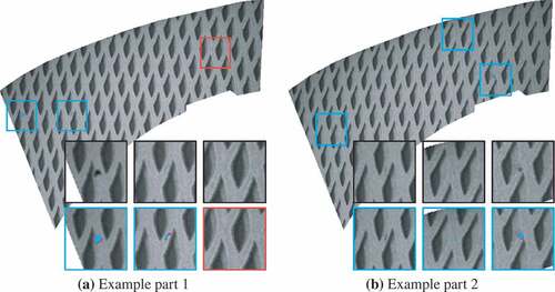
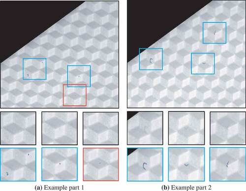
Figure 6. Two parts of dataset A with view on the same section. Defect-wise true positives (blue squares) and false positives (red squares) detected by the FCN are superimposed. At pixel level, blue pixels indicate true positive predictions, red pixels indicate false positives and purple pixels indicate false negatives.

The process of surface inspection can be divided into three steps. First, the acquisition of surface images, which includes appropriate part handling and surface illumination to ensure that occurring defects become visible in the surface images. Second, the detection and localization of anomalies in the acquired images. Third, the assessment of the visual perceptibility of each detected defect. The focus of this work is on the second step. The challenge of detecting defects on surface images strongly depends on the appearance of the fault-free surface images. While for homogeneous, non-patterned surfaces, defective patterns can be directly segmented from fault-free regions by (adaptive) thresholding, there is far more effort needed for surfaces that show a complex normal appearance such as patterned or decorated surfaces. In this regard, algorithms need to distinguish allowed structures from non-allowed or defective ones. A particular challenge are images of patterned surfaces that show significant sample-to-sample variations, such as those in Figure 1. Such types of surface images are treated in this work. Since in this case every instance is unique, no single part can be used as a “golden sample”. Rather, the entire range of permitted variations must be covered by the method to enable differentiation between allowed variations and defects.

Figure 1. Surface images of two different samples used in the case study. Note that although the two images show the exact same sample region, significant appearance variations are recognizable. The reason is variations in the pattern primitives and slightly changed global pattern distortion and positioning. The right image shows a pixel-wise annotated defect.

The detection of defects in surface images can be considered as the detection of local visual anomalies. Anomaly detection means the detection of patterns that deviate from the expected appearance, which in case of surface inspection, can be indirectly defined by a set of samples that are classified as fault-free by a human. Anomaly detection is closely related to novelty detection, which focuses on the detection of previously unseen patterns (Chandola, Banerjee, and Kumar 2009). In both cases, after a model is built from normal (fault-free) data, it is used to detect anomalous or novel instances in the test data. Regarding surface inspection, small and weakly contrasted anomalies are a particular challenge, since they do not change the overall semantic of an image and are often obscured by allowed appearance variations.

Machine learning defect detection models that are trained in a purely supervised manner usually perform better than unsupervised one-class approaches. However, in addition to normal instances, they also require faulty ones for training. For surface inspection, however, it is difficult to provide a substantial number of faulty instances. One reason is that certain defect types simply occur very rarely, which requires extensive manual image assessment in order to acquire a sufficient number of examples. Furthermore, the effort for the pixel-wise annotation of defects on a multitude of images is huge. In this paper, this issue is circumvented by synthesizing defects, which are then injected into fault-free image patches. One-class (fault-free) data is thereby transformed into two class data, on which a supervised model can be trained. This way, the performance of supervised approaches can be utilized without the need for manually labeled multi-class data.

Related Work

There exist several reviews about anomaly detection, novelty detection and texture analysis that refer to methodologies that are suitable for surface inspection (Chandola, Banerjee, and Kumar 2009; Huang and Pan 2014; Kwon et al. 2017; Neogi, Mohanta, and Dutta 2014; Pimentel et al. 2014; Xie 2008), some of which are domain-specific and can not easily be applied under different circumstances. Regarding patterned surface images, Tsai, Chuang, and Tseng (2007) used filters in the frequency domain to remove periodic structural patterns for automatic defect inspection of TFT-LCD panels. With this approach, however, false alarms are unavoidable if random distortions in the pattern are allowed. Another possibility when facing randomly distorted patterns is to compute a virtual golden sample for every inspected surface image by replacing every single pattern primitive by its neighbors in consideration of the local distortion (Haselmann and Gruber 2016). This, however, is limited to regularly arranged patterns that do not exceed distortions that would result in a non-linear warping between neighbored pattern primitives. There also exist methods that are designed for detecting anomalies in more irregular patterns. For example, Alimohamadi, Ahmadyfard, and Shojaee (2009) and Ralló, Millán, and Escofet (2009) used methods based on Gabor filtering to detect defects in textiles. The focus in these cases is on rather pronounced defects and not on very weak ones, such as the ones treated in the present work. Another category of surface inspection methodology is based on statistical features such as histogram analysis (Iivarinen 2000; Ng 2006) or co-occurrence matrices (Bodnarova et al. 1997; Choudhury and Dash 2018; Iivarinen, Rauhamaa, and Visa 1996).

Learning-based methods are of particular interest in complex inspection tasks. Although corresponding models are trained with domain-specific examples, the underlying architecture of the models can still be used without major changes for other application domains. However, this assumes that no handcrafted, domain-specific features are used. Since the rise of deep learning, however, manually engineered features are no longer necessarily an advantage. In fact, modern deep learning architectures surpass conventional ML-learning methods in the majority of pattern recognition tasks and even achieve superhuman performance in some of them without using any handcrafted features. With regard to defect detection, however, the main problem with supervised deep learning is the large number of normal and faulty samples necessary for training. There exist strategies to attenuate this problem, such as transfer learning and extensive virtual data augmentation. Nevertheless, in many scenarios, where only a few faulty image patches are available alongside thousands of normal ones, supervised training remains a challenge.

One way to avoid the issue of providing a sufficient number of positive samples is machine learning methods that are trained in an unsupervised way on exclusively normal data. For example, Zhang et al. (2017) used a convolutional neural network (CNN) as a one-class classifier to map instances into a certain feature space, in which the mapped instances were clustered within a hypersphere. While this approach worked well for the detection of instances that semantically strongly deviated from the normal ones, weakly deviating instances were often misclassified. Kholief, Darwish, and Fors (2017) experimented with autoencoders for defect detection on steel surfaces. Xu et al. (2016) worked with stacked sparse autoencoders to detect nuclies on breast cancer histopathology images. Mei, Wang, and Wen (2018) investigated convolutional denoising autoencoders for automatic fabric defect detection. Another recent approach was proposed by Schlegl et al. (2017), where generative adversarial networks are trained on normal instances. The generative network is then used to generate an instance that looks as similar as possible to the inspected image patch. The (pixel-wise) similarity between the two images is used as an (pixel-wise) anomaly score.

Regarding synthetized data, research is conducted in various image processing related areas. Theiler and Cai (2003) used a resampling scheme to produce a “background class” from multispectral landscape images where binary classification is then used to distinguish the original training instances from the background. In a more recent example, a large data set with accurate pixel-level labels was generated with the help of computer games (Richter et al. 2016). The injection of local anomalies into fault-free patterned surface images has recently been demonstrated, whereby a convolutional neural network could then be trained to detect real defective image patches (Haselmann and Gruber 2017). The corresponding defect synthetization algorithm is slightly modified and used in the present paper, where instead of patch-wise classification, pixel accurate defect detection is demonstrated. On the considered surface images, the proposed method clearly surpasses the tested state of the art unsupervised anomaly detection method.

Methodology

Pre- and Post Processing Pipeline

The raw input data fed into the image processing pipeline are high-resolution surface images with up to $2448\times 2050$ pixels, each showing certain areas of a fabricated part. Multiple pre-defined viewing directions are necessary to cover the whole surface of the free-formed plastic parts (for details see section 4.1). For each viewing direction, the parts are placed in the same position, with the exception of small variations caused by the handling system. In addition to these small positioning variations, the detail characteristic of the surface decoration may vary from part to part. For each pre-defined (high-resolution) viewing direction, a mask is defined that separates the visible part surface from occurring background. The visible background in the acquired surface images is blackened with the help of these defined masks.

In order to prepare the raw input data for a typical convolutional neural network, patches of size $64\times 64$ are extracted from the high-resolution surface images. In addition, $64\times 64$ patches are extracted from the corresponding high-resolution masks and used as additional network input. In the next step, synthetic defects (Haselmann and Gruber 2017) (discussed in section 3.2) are injected into 50% of the raw patches, which are considered as fault-free by definition. Since the synthetization algorithm considers only one image channel, RGB input images have to be processed separately for each color channel. This is followed by data augmentation including rotation, zooming, shear, etc. This, however, can lead to unwanted border effects, which is avoided by initially extracting auxiliary patches of size $100\times 100$. After applying transformations for data augmentation, the patches are center-cropped to the target size of $64\times 64$. Due to the injection of artificial defects, for each preprocessed patch the pixel-wise ground truth (the pixel-wise location of the injected defects) is known. As a consequence, supervised learning models can be trained to detect defects with pixel accuracy, which is an image processing task generally known as image segmentation.

During the training phase, the preprocessing pipeline is performed in real time in order to maximize the variations between training patches in three respects:

• Every possible raw patch is extracted from the input training images considering shifts of the extraction window pixel by pixel. There is a very large number of possible extraction window locations (figures regarding both tested data sets are provided in section 4.1). During each training cycle, all possible locations are extracted in random order. Although the resulting patches are strongly correlated, this can be considered as a form of data augmentation (besides the additional data augmentation at the end of the preprocessing pipeline).

• Every injected synthetic defect is newly generated by a stochastic process (Haselmann and Gruber 2017) (discussed in section 3.2) with the aim to achieve high defect variability.

• The random data augmentation is performed independently for each processed patch.

By these techniques, the neural network almost certainly never sees two identical patches.

For the validation data, a fixed set of patches is extracted from unseen fault-free samples at random positions. Similarly, as for the training set, synthetic defects are injected into 50% of the extracted patches. Because no real defects are annotated, it is not possible with this data set to fully evaluate the generalization capability of a fitted model. However, it can be tested whether the model generalizes well to unseen surface images including unseen decorative features.

The test set is based on an unseen set of images where occurring real defects are manually labeled on pixel level. Patches are extracted according to a grid with a space interval of 20 pixels. Such an interval results in each surface section being seen multiple times, except for some corner regions. After inference, the predictions are merged again according to the grid, wherein overlapping regions the predicted maximum probability is selected for each pixel.

Synthetization of Artificial Defects

For the synthetization of artificial defects, the algorithm of an earlier work (Haselmann and Gruber 2017) is used in a slightly modified version in the given paper. The algorithm synthesizes defects with a large variety (see Figure 2). The purpose of such a wide distribution of artificial defects is that they are likely to cover most of the occurring real defects.

Figure 2. Stepwise injection of synthetic defects on fault-free image patches. The first image row shows the fault-free image patch to be manipulated. The second shows randomly generated defect skeletons. The third row shows the random textures created on this basis. The fourth row shows the query image with the injected artificial defect. The fifth shows the difference image between the query and its manipulated version. The sixth row shows the ground truth provided for the network training.

The defect synthetization algorithm can be roughly divided into four steps. First, a random binary defect skeleton is generated by means of a stochastic process that resembles a random walk with momentum. In the second step, a random texture is generated on basis of the skeleton. For this purpose, the skeleton points are first replaced by gray values. Afterward, the image is blurred to obtain a thicker defect morphology. In the third step, the randomly generated defect texture is used to modify a (fault-free) image patch of the one-class training data. Each of these first three steps of the algorithm is subject to several random variables (Haselmann and Gruber 2017), which helps to achieve high variability of artificial defects. This not only leads to very diverse defect morphologies (skeletons that are straight, restless, jagged, curved, angular, circular, bulky, or various mixtures thereof) but also to different defect characteristics in terms of contrast and intensity progression. For example, a bright–dark transition in the normal structure can (controlled by a random variable) lead to an interruption of the artificial defect in some cases.

The distribution of each random variable of the defect synthetization algorithm is determined by several hyperparameters (Haselmann and Gruber 2017), which can be adjusted according to the specific defect detection task. For example, a model can be trained to distinguish line-like defects from bulky defects by using two sets of hyperparameters that result in two different groups of morphologies. In this work, however, no differentiation between defect types has been pursued. In order to achieve a high variability of defects, a rather broad distribution for each random variable has been chosen (see Figure 2).

In the fourth step, the visibility of the synthesized defects is analyzed. For some realizations of the random variables, the generated artificial defects are barely visible or not visible at all. Those image patches are discarded according to a predefined visibility limit. Furthermore, in the fourth step, the defect visibility is analyzed pixel-wise to generate pixel-level labels for the conducted experiments.

Network Architecture

A fully convolutional network (FCN) according to Jonathan Long, Shelhamer, and Darrell (2015) was used for defect segmentation (see Figure 3).

Encoder

For the encoder part – (64C3-128C3-MP2)-(128C3-128C3-MP2)-(128C3-128C3-MP2)-(2C1) – eight convolutional layers were used, whereby after the second, fourth and sixth layer max-pooling was applied. As the input size of the network is $64\times 64$, this results in a feature map size of $8\times 8$ after max-pooling in the sixth layer. In the seventh layer, a $1\times 1$ kernel was used for dimensionality reduction. Rectified Linear Units (ReLUs) were used as activation functions for each layer in the encoder with batch normalization applied prior to them.

Decoder

The decoder part of the segmentation network consists of two layers that upsample their corresponding input regions by transposed convolution with strides 2 and 4, respectively. In favor of a better segmentation granularity, there is a skip connection from the output of the first upsampling layer to the output of the fourth layer of the encoder part. For the decoder part, linear activations were used without batch normalizations.

Training Details

The fully convolutional network (FCN) was trained from scratch using the ADAM optimizer [13] with hyperparameters $\alpha =0.0005$, ${\beta }_1=0.9$, ${\beta }_2=0.999$, $ϵ={10}^{-8}$ and a batch size of 336. In all layers, the weights were initialized from a truncated Gaussian distribution with a mean of 0 and a standard deviation of 1. All biases were zero-initialized.

Metrics for Model Evaluation on Imbalanced Data Sets

Despite the injection of synthetic defects, which leads to patch-wise balanced training and validation data, there is a strong imbalance at pixel level, since the majority of pixels is negative. The test data set is imbalanced even when considering patch-wise classification, because no synthetic defects but only real ones occur. The imbalance of data sets is commonly represented by its skew,

(1) $Skew=\frac{negatives}{positives},$(1)

where negatives denote the number of fault-free (negative) instances and positives the number of defective (positive) instances. On highly skewed data sets, some metrics can be misleading. One such example is the commonly used accuracy that reaches values close to $1$ for a model that predicts every instance to be negative.

Receiver-Operator-Characteristic (ROC)

Another common metric is the ROC curve and the area under it (AUROC). The ROC curve is a plot of the recall (true positive rate),

(2) $Recall=\frac{\mathrm{T}\mathrm{P}}{\mathrm{T}\mathrm{P}+\mathrm{F}\mathrm{N}},$(2)

against the false-positive rate (FPR),

(3) $\mathrm{F}\mathrm{P}\mathrm{R}=\frac{\mathrm{F}\mathrm{P}}{\mathrm{F}\mathrm{P}+\mathrm{T}\mathrm{N}},$(3)

at various threshold settings, where $\mathrm{T}\mathrm{P}$ is the number of true positives, $\mathrm{F}\mathrm{P}$ is the number of false positives, $\mathrm{F}\mathrm{N}$ is the number of false negatives and $\mathrm{T}\mathrm{N}$ is the number of true negatives. In contrast to accuracy, a model that predicts all pixels to be negative does not surpass the AUROC baseline of 0.5. ROC metrics might therefore be suitable to assess the performance of tested models on data sets with a large skew. However, for reasonably well-performing models, applied on a data set with a very high skew, the ROC curve rises sharply due to the large fraction of $\mathrm{T}\mathrm{N}$ which leads to an AUROC close to $1$. Therefore, ROC metrics can be misleading for the comparison of two well-performing models on strongly imbalanced data sets (Davis and Goadrich 2006; Jeni, Cohn, and de La Torre 2013). Nevertheless, for the sake of completeness, ROC and AUROC are reported on pixel level.

Precision-Recall-Curve (PRC)

For data sets with a large fraction of negative instances, metrics such as precision in combination with recall are frequently reported. One defines precision as

(4) $Precision=\frac{\mathrm{T}\mathrm{P}}{\mathrm{T}\mathrm{P}+\mathrm{F}\mathrm{P}}.$(4)

In contrast to the ROC metrics, precision and recall are not affected by a large fraction of $\mathrm{T}\mathrm{N}$. Actually, it is also possible to evaluate problems where no or no meaningful counting of $\mathrm{T}\mathrm{N}$ is possible. Precision-recall metrics are therefore very sensitive when comparing models on data sets (Davis and Goadrich 2006) with a large skew, such as in the given case. While for balanced data sets the baseline of the AUPRC is also about $0.5$, for data sets with a large skew the baseline approaches zero.

Matthews Correlation Coefficient (MCC)

The MCC (Matthews 1975) is another metric that will be reported in this paper:

(5) $\mathrm{M}\mathrm{C}\mathrm{C}=\frac{\mathrm{T}\mathrm{P}\cdot \mathrm{T}\mathrm{N}-\mathrm{F}\mathrm{P}\cdot \mathrm{F}\mathrm{N}}{{\left((\mathrm{T}\mathrm{P}+\mathrm{F}\mathrm{P})(\mathrm{T}\mathrm{P}+\mathrm{F}\mathrm{N})(\mathrm{T}\mathrm{N}+\mathrm{F}\mathrm{P})(\mathrm{T}\mathrm{N}+\mathrm{F}\mathrm{N})\right)}^{1/2}}.$(5)

The MCC is between $-1$ and $1$, whereas 0 is the baseline for random prediction. An MCC of 1 corresponds to a perfect prediction. In contrast, $-1$ corresponds to a prediction that is exactly the wrong way around. For imbalanced classification problems, especially those with low skew, the $\mathrm{M}\mathrm{C}\mathrm{C}$ is regarded as more meaningful than the ${\mathrm{F}}_1$ score, because it takes into account the balance ratios of all four categories of the confusion matrix (Chicco 2017).

Defect-Wise Evaluation

In addition to the pixel-wise evaluated metrics, the AUPRC is reported considering defect-wise detection. The defect-wise $\mathrm{T}\mathrm{P}$, $\mathrm{F}\mathrm{P}$ and $\mathrm{F}\mathrm{N}$ are defined as follows: A correctly detected defect ($\mathrm{T}\mathrm{P}$) is counted if at least one associated pixel has been classified as defect-positive. Otherwise, it is counted as an undetected defect ($\mathrm{F}\mathrm{N}$). A false-positive occurrence ($\mathrm{F}\mathrm{P}$) is counted whenever a cluster (connected components whose pixels are connected through an 8-pixel connectivity) of positive predicted pixels does not include any positively labeled pixels. True negatives $\mathrm{T}\mathrm{N}$, in turn, can not be reasonably counted on a defect basis. AUROC and MCC, can therefore not be reported on a defect basis.

Experiments

Data Sets

The images used for the case study originate from free-form plastic parts whose surface decoration significantly varies from part to part. Multiple views per part were necessary to cover the entire surface. However, the positioning of the parts is fixed for each view, with the exception of small variations (see Figure 1). Two different types of parts were used for the experiments, resulting into two data sets, called A and B. On data set A, a state of the art unsupervised anomaly detection method (Schlegl et al. 2017) was tested for reasons of comparison. All parts of each data set were split up into three groups (Training, Validation, and Test).

As already stated in section 3.1, it is assumed that the raw training and validation data are fault-free. Patches labeled as positive are only provided by injecting synthetic defects. Hence, the parts that showed noticeable defects were used for the test set. The other parts were used for the training set and validation set. While the parts used for training and validation are not completely fault-free, they appear to be so at first glance. Only in the test set, visible defects were manually annotated. Data set A includes four viewing directions per part, whereas 34 parts were used for training, 9 for validation and 17 for testing with real defects. All four viewing directions combined, a total of 1055862 different image patches can be extracted per part, which are strongly overlapping. Since the patch size was chosen to be of size $64\times 64$, this results in approximately 260 non-overlapping image patches per part. For data set B, which contains three viewing directions per part, 12 parts were used for training, 12 for validation and 4 for testing.

Results

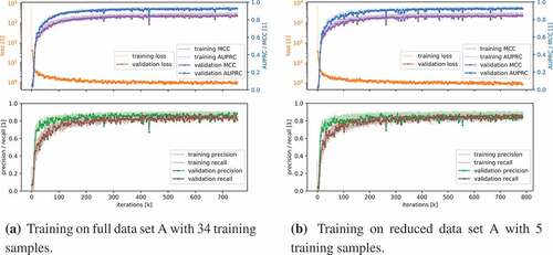
The results for data set A are summarized in Table 1. The corresponding PR and ROC curves are shown in Figure 4. All models of the FCN network (see Figure 3) were trained on 300k to 700k batches with synthetic defects until the AUPRC saturated on the validation data set (see Figure 5). According to the loss and the segmentation AUPRC history for training and validation, neither significant under- nor over-fitting occurred. This also holds true when training is performed on a subset of data set A consisting of only five parts for training. Presumably, this is made possible by the extensive data augmentation both on basis of raw data and with regard to synthesized defects that are used only once.

Table 1. Summary of results.

	Pixel-wise			Defect-wise
	AUPRC	AUROC	MCC	AUPRC	TP	FP	FN
FCN (data set A)	0.78	0.9999	0.65	0.77	64	145	3
FCN (five parts of A)	0.75	0.9998	0.61	0.77	61	127	6
AnoGAN (data set A)	0.08	0.84
FCN (data set B)	0.76	0.9997	0.67	0.87	302	225	30

Figure 4. ROC and PR curves for data set A. The areas under the curves are reported within the parenthesis.

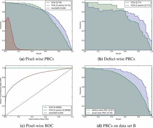
Figure 3. Architecture of the fully convolutional neural network (FCN). The orange cuboids represent convolutional layers (conv.) with kernels of size 3 × 3 with downstreamed batch normalization (BN) and rectified linear units (ReLU) as activation function. The yellow cuboids represent layers that upsample its input by transposed convolution with strides 2 and 4.

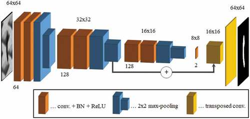
Figure 5. Training history of the fully convolutional neural network on data set A.

Full Training Set A

On data set A, consisting of 34 parts, a segmentation AUPRC of 0.78 was reached on the test set (which includes manually annotated real defects) in comparison to 0.92 on the validation data set (which includes only synthetic defects). Considering the patch-wise AUPRC, a score of 0.77 (test) and 0.97 (validation) was achieved. Examples of surface images of test data set A with superimposed CNN predictions are shown in Figure 6.

It is noteworthy that the AUPRC is much lower on the test data sets than on the validation data sets. This can be explained by fact that the test set has a much higher skew than the validation set. While 50% of the patches in the validation data set contain defects, this holds true for only about 0.5% of the patches in the test data set. On pixel level the situation is similar: 0.4% of the pixels are positive in the validation data set in comparison to only 0.004% in the test data set. This ratio of 100 between the skew of the test data set and the validation data set strongly affects the measured AUPRC, as also demonstrated by Jeni, Cohn, and de La Torre (2013).

Since slightly imperfect structures appear in the raw training data set, which is defined to be fault-free, it is difficult, if not impossible, to draw a sharp line between defect and non-defect. The majority of negatively labeled patches on which at least one pixel was predicted as positive (see Figure 7a), showed structures that could be interpreted as defects.

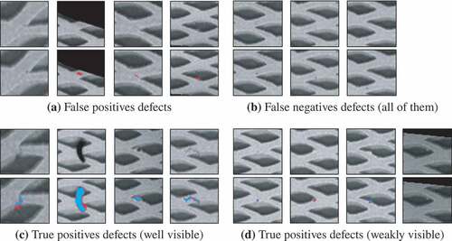
Figure 7. Examples of image patches of data set A (upper row) with merged predictions (lower row). At pixel level, blue pixels indicate true positive predictions, red pixels indicate false positives and purple pixels indicate false negatives. The contrast of undetected defects in (a) resembles the contrast of false positively detected structures in (b). This is a consequence of the problem that no sharp line between a defect and non-defect can be drawn.

Reduced Training Set A (Five Parts Only)

With the repetition of the experiments on the significantly reduced data set, the performance of the models hardly deteriorated. The segmentation PRC scores of 0.75 (test) and 0.94 (validation), as well as the patch-wise PRC scores of 0.77 (test) and 0.93 (validation), were just slightly below the scores of the models trained on the full data set.

Comparison to AnoGANs

As a comparison, an unsupervised anomaly detection method utilizing a generative adversarial network (AnoGAN) (Schlegl et al. 2017) was tested (similar comparison has been performed by Haselmann et al. 2018). For this, the publicly available implementation of Ayad et al. (2017) was used. The GAN was trained on the full training set without the injection of synthetic defects, thus only on fault-free patches. After training, the GAN was used to generate patches that were as similar as possible to the patches of the test data set. As proposed by Schlegl et al. (2017) this was done by mapping the corresponding patches to the latent space of the network by an iterative optimization process. Since this resulted in an inspection time that was 60000 times longer compared to the inspection time of the FCN, AnoGANs were only tested on one data set (data set A).

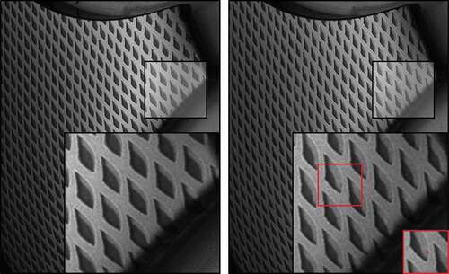
It turned out that the images generated by the GAN did not match the query images very well when trained on patches containing visible edges of the defined regions of interest (ROIs). Therefore, the GAN was retrained (and tested) on patches with no visible mask edges (see Figure 8). Although the majority of generated patches looked quite realistic, only a segmentation AUPRC of 0.08 could be reached. Non-matching reconstructions, such as in Figure 8d, were excluded for reasons of comparability since there were presumably a result of the optimization procedure for the being stuck in a local minimum in the latent space. Nevertheless, only the few most high-contrast defects, such as the one in Figure 8b were reliably detected. Weakly contrasted defects, such as in Figure 8c were often mixed up with normal structures.

Figure 8. Examples of four image patches processed by AnoGANs as a comparison to the proposed method. The top row shows image patches to be inspected (query images). The middle row shows the reconstructions by the AnoGAN. The bottom row shows the absolute value of the difference image between the query and reconstructed image. While column (a) shows a fault-free image patch, (b) and (c) show an image patch with a strongly visible and weakly visible defect, respectively. Failed reconstructions, such as in (d) have been discarded in order to enhance the measured pixel-wise AUPRC and AUROC.

Training Set B

Similarly to the results on data set A, the FCN reached a pixel-wise AUPRC of 0.76 for the test set and 0.97 for the validation set. Defect-wise, the AUPRCs were at 0.87 (test) and 0.99 (validation). Surface images of data set B including highlighted defects are depicted in Figure 9.

Figure 9. Two parts of dataset B with view on the same section. Defect-wise true positives (blue rectangulars) and false positives (red rectangular) detected by the FCN are superimposed. At pixel level, blue pixels indicate true positive predictions, red pixels indicate false positives and purple pixels indicate false negatives.

Discussion

On data set A, the pixel-wise AUPRC of 0.78 – reached by the proposed method – is much higher than the AUPRC of 0.08 of the tested state-of-the-art unsupervised anomaly detection method. One of the reasons for this is that weakly contrasted defects, such as those depicted in Figure 7d, were only detected by the proposed method. This is not surprising, as the sensitivity of the method is significantly influenced by the distribution of the artificial defects. Furthermore, it could be shown that a similarly good performance (pixel-wise AUPRC of 76%) could be reached even when training was performed on five surface samples only. For surface inspection, this means that the effort for teaching a new type of surface to the system is low.

The limitations of the described method are dictated by the injection of synthetic defects. Defects that are not covered by the distribution of artificial ones cannot be reliably detected. Especially anomalies that are only visible when looking at a larger area of the surface can hardly be detected since they are difficult to synthesize. However, in some cases, a multi-scale version of the described method – where the input images are scaled to different sizes in order to cover defects of strongly varying sizes – might work. Another limitation occurs for RGB images. Since the injection of synthetic defects is based on gray levels, the RGB channels cannot be jointly analyzed. They have to be processed independently, either with one model for all channels or with a separate model for each channel.

Conclusion

In this paper, a method is proposed that is capable of detecting locally confined defects on surface images with pixel accuracy. The method uses a fully convolutional neural network for image segmentation that is trained on respective surface images that have been defined as fault-free by the user. For this purpose, image patches are randomly extracted from the high-resolution surface images. In order to enable two-class supervised training on a pixel basis, randomly generated artificial defects are injected into 50% of the extracted patches. Consequently, real defects are not required for training. By these means the common issue in machine learning driven surface inspection of collecting and labeling sufficient amounts of data can be bypassed. Experiments were conducted on two different data sets. On data set A, a pixel-wise AUPRC (area under the precision–recall curve) of 78% was achieved, compared to the AUPRC of 8% of a state-of-the-art unsupervised anomaly detection method. Furthermore, it could be shown that a similarly good performance (pixel-wise PRC score of 76%) could be achieved even when training was performed on five surface samples only.

Acknowledgments

The research work of this paper was performed at the Polymer Competence Center Leoben GmbH (PCCL, Austria) within the framework of the COMET-program of the Federal Ministry for Transport, Innovation and Technology and the Federal Ministry of Digital and Economic Affairs with contributions by Burg Design GmbH, HTP High Tech Plastics GmbH, and Schöfer GmbH. The PCCL is funded by the Austrian Government and the State Governments of Styria, Lower Austria and Upper Austria.

Additional information

Funding

This work was supported by the Austrian Research Promotion Agency (FFG) [grant number 858676].

References

- Alimohamadi, H., A. Ahmadyfard, and E. Shojaee. 2009. Defect detection in textiles using morphological analysis of optimal gabor wavelet filter response. 2009 International Conference on Computer and Automation Engineering, 26–30. IEEE. doi:10.1109/ICCAE.2009.43.
- Ayad, A., M. Shaban, and W. Gabriel. 2017. Unsupervised Anomaly Detection with Generative Adversarial Networks on MIAS dataset. Accessed June 11 , 2018. https://github.com/xtarx/Unsupervised-Anomaly-Detection-with-Generative-Adversarial-Networks.
- Bodnarova, A., J. A. Williams, M. Bennamoun, and K. K. Kubik. 1997. Optimal textural features for flaw detection in textile materials. Proceedings of IEEE TENCON '97 - Brisbane, Australia. IEEE Region 10 Annual Conference. Speech and Image Technologies for Computing and Telecommunications, ed. M. Deriche, M. Moody and M. Bennamoun, 307–10. New York, NY, USA, IEEE. doi:10.1109/TENCON.1997.647318.
- Chandola, V., A. Banerjee, and V. Kumar. 2009. Anomaly detection: A survey. ACM Computing Surveys 41: doi: 10.1145/1541880.1541882.
- Chicco, D. 2017. Ten quick tips for machine learning in computational biology. BioData Mining 10:35. doi:10.1186/s13040-017-0155-3.
- Choudhury, D. K., and S. Dash. 2018. Defect detection of fabrics by grey-level co-occurrence matrix and artificial neural network. In Handbook of research on modeling, analysis, and application of nature-inspired metaheuristic algorithms, 285–97. doi:10.4018/978-1-5225-2857-9.ch014.
- Davis, J., and M. Goadrich. 2006. The relationship between precision-recall and ROC curves. Proceedings of the 23rd international conference on machine learning - ICML ’06, ed. W. Cohen and A. Moore, 233–40. New York, NY: ACM Press. doi:10.1145/1143844.1143874.
- Haselmann, M., and D. Gruber. 2017. Supervised machine learning based surface inspection by synthetizing artificial defects. 2017 16th IEEE international conference on machine learning and applications (ICMLA), 390–95. IEEE. doi:10.1109/ICMLA.2017.0-130.
- Haselmann, M., and D. P. Gruber. 2016. Anomaly detection on arbitrarily distorted 2D patterns by computation of a virtual golden sample. 2016 IEEE international conference on image processing (ICIP), 4398–402. IEEE. doi:10.1109/ICIP.2016.7533191.
- Haselmann, M., D. P. Gruber, and P. Tabatabai. 2018. Anomaly Detection Using Deep Learning Based Image Completion, International Conference on Machine Learning and Applications (ICMLA) - Orlando, Florida, USA. 1237–1242. New York, NY, USA, IEEE. doi:10.1109/ICMLA.2018.00201
- Huang, S.-H., and Y.-C. Pan. 2014. Automated visual inspection in the semiconductor industry: A survey. Computers in Industry 66:1–10. doi:10.1016/j.compind.2014.10.006.
- Iivarinen, J. 2000. Surface defect detection with histogram-based texture features. In Intelligent robots and computer vision XIX: algorithms, techniques and active vision, ed. D. P. Casasent. 140–45. Bellingham, Washington, USA, SPIE. doi:10.1117/12.403757.
- Iivarinen, J., J. Rauhamaa, and A. Visa. 1996. Unsupervised segmentation of surface defects. Proceedings of 13th international conference on pattern recognition, vol. 4, 356–60. IEEE. doi:10.1109/ICPR.1996.547445.
- Jeni, L. A., J. F. Cohn, and F. de La Torre. 2013. Facing imbalanced data: recommendations for the use of performance metrics. International conference on affective computing and intelligent interaction and workshops: [proceedings]. ACII (conference) 2013, 245–51. doi:10.1109/ACII.2013.47.
- Kholief, E. A., S. H. Darwish, and N. Fors. 2017. Detection of steel surface defect based on machine learning using deep auto-encoder network. In Industrial engineering and operations management, ed. A. Ali and I. Kissani. IEOM Society. 218–29.
- Kwon, D., H. Kim, J. Kim, S. C. Suh, I. Kim, and K. J. Kim. 2017. A survey of deep learning-based network anomaly detection. Cluster Computing 9:205. doi:10.1007/s10586-017-1117-8.
- Long, J., E. Shelhamer, and T. Darrell. 2015. Fully convolutional networks for semantic segmentation. Conference of computer vision and pattern recognition (CVPR) - Boston, MA, USA, 1–8. New York, NY, USA, IEEE. doi:10.1109/CVPR.2015.7298965
- Matthews, B. W. 1975. Comparison of the predicted and observed secondary structure of T4 phage lysozyme, Biochimica et Biophysica Acta (BBA). Protein Structure 405:442–51. doi:10.1016/0005-2795(75)90109-9.
- Mei, S., Y. Wang, and G. Wen. 2018. Automatic fabric defect detection with a multi-scale convolutional denoising autoencoder network model. Sensors (Basel, Switzerland) 18:1064. doi:10.3390/s18041064.
- Neogi, N., D. K. Mohanta, and P. K. Dutta. 2014. Review of vision-based steel surface inspection systems. EURASIP Journal on Image and Video Processing 50:3. doi:10.1186/1687-5281-2014-50.
- Ng, H.-F. 2006. Automatic thresholding for defect detection. Pattern Recognition Letters 27:1644–49. doi:10.1016/j.patrec.2006.03.009.
- Pimentel, M. A., D. A. Clifton, L. Clifton, and L. Tarassenko. 2014. A review of novelty detection. Signal Processing 99:215–49. doi:10.1016/j.sigpro.2013.12.026.
- Ralló, M., M. S. Millán, and J. Escofet. 2009. Unsupervised novelty detection using gabor filters for defect segmentation in textures. Journal of the Optical Society of America A 26:1967. doi:10.1364/JOSAA.26.001967.
- Richter, S. R., V. Vineet, S. Roth, and V. Koltun, Playing for data: ground truth from computer games, 2016. Accessed http://arxiv.org/pdf/1608.02192v1.
- Schlegl, T., P. Seeböck, S. M. Waldstein, U. Schmidt-Erfurth, and G. Langs. Unsupervised anomaly detection with generative adversarial networks to guide marker discovery, 2017. Accessed: http://arxiv.org/pdf/1703.05921v1.
- Theiler, J. P., and D. M. Cai. 2003. Resampling approach for anomaly detection in multispectral images. SPIE proceedings, Proc. SPIE 5093, Algorithms and Technologies for Multispectral, Hyperspectral, and Ultraspectral Imagery IX - Orlando, Florida, USA, ed. S. S. Shen and P. E. Lewis, 230. SPIE. doi:10.1117/12.487069.
- Tsai, D.-M., S.-T. Chuang, and Y.-H. Tseng. 2007. One-dimensional-based automatic defect inspection of multiple patterned TFT-LCD panels using Fourier image reconstruction. International Journal of Production Research 45:1297–321. doi:10.1080/00207540600622464.
- Xie, X. 2008. A review of recent advances in surface defect detection using texture analysis techniques. Electronic Letters on Computer Vision and Image Analysis 7:1–22. doi:10.5565/rev/elcvia.268.
- Xu, J., L. Xiang, Q. Liu, H. Gilmore, J. Wu, J. Tang, and A. Madabhushi. 2016. Stacked sparse autoencoder (SSAE) for nuclei detection on breast cancer histopathology images. IEEE Transactions on Medical Imaging 35:119–30. doi:10.1109/TMI.2015.2458702.
- Zhang, M., J. Wu, H. Lin, P. Yuan, and Y. Song. 2017. The application of one-class classifier based on CNN in image defect detection. Procedia Computer Science 114:341–48. doi:10.1016/j.procs.2017.09.040.