Anomaly Detection in Power Generation Plants Using Machine Learning and Neural Networks

ABSTRACT

The availability of constant electricity supply is a crucial factor to the performance of any industry. Nevertheless, the unstable supply of electricity in Cameroon has led to countless periods of electricity load shedding, hence, making the management of the telecom industry to fall on backup power supply such as diesel generators. The fuel consumption of these generators remain a challenge due to some perturbations in the mechanical fuel level gauges and lack of maintenance at the base stations resulting to fuel pilferage. In order to overcome these effects, we detect anomalies in the recorded data by learning the patterns of the fuel consumption using four classification techniques namely; support vector machines (SVM), K-Nearest Neighbors (KNN), Logistic Regression (LR), and MultiLayer Perceptron (MLP) and then compare the performance of these classification techniques on a test data. In this paper, we show the use of supervised machine learning classification based techniques in detecting anomalies associated with the fuel consumed dataset from TeleInfra base stations using the generator as a source of power. Here, we perform the normal feature engineering, selection, and then fit the model classifiers to obtain results and finally, test the performance of these classifiers on a test data. The results of this study show that MLP has the best performance in the evaluation measurement recording a score of $96\mathrm{\%}$ in the K-fold cross validation test. In addition, because of class imbalance in the observation, we use the precision-recall curve instead of the ROC curve and registered the probability of the Area Under Curve (AUC) as $0.98$.

Introduction

The expansion of mobile services of the telecommunication industries has resulted in the installation of cell towers to diverse parts of the world. In developing countries like Cameroon, the supply of the power grid is irregular and the network companies find it difficult to manage their base stations particularly, their data centers and other IT equipments. Due to this, the management of the base stations uses backup power supply such as diesel generators, solar panels, batteries and other secondary source of power to keep their systems in operation. However, these backup sources, particularly, the power generation plants have also created additional complications like external or internal seeps of oil, fuel or coolant, inaccuracies in the mechanical fuel level gauges and poor maintenance leading to fuel pilferage from the various base stations of the network operators. These anomalies directly increase the fuel consumption and affect the operations of the industry in the long run. Therefore, our goal in this work, is to adopt machine learning (ML) scheme, using TeleInfra¹ as a case study to identify the anomaly in fuel consumption of their standby generators.

TeleInfra is a telecommunication company in Cameroon that uses backup generators when the main power grid goes down. The company provides services such as site maintenance and refueling of generators in the base stations. The dataset used in this paper is obtained from base stations under supervision of TeleInfra company. It contains attributes of fuel consumed by the generators and other information such as maintenance details.

Anomaly in a data is considered as an observation which does not conform to the expected standard in the data. Meanwhile, recent works in anomaly detection such as fraud detection analysis (Chouiekh and EL Hassane 2018; Zanin et al. 2018), thermal power plant (Banjanovic-Mehmedovic et al. 2017), medical image analysis (Taboada-Crispi et al. 2009), etc., have shown how well ML techniques can be used to address these challenges.

From the various anomaly detection researches, the algorithms used can outperform each other based on the type of data and the underlying assumptions employed. From the literature, most of the competitive ML techniques used in classification task like in our case, consist of SVM², KNN³, LR⁴, and MLP⁵. In this study, we do a comparative analysis of the performance of these classifiers to determine the best classifier that can accurately detect the anomalies in the fuel consumption dataset. SVM aims at generating an optimal hyperplane (decision plane) that maximizes the margin between two classes, using support vectors. KNN stores the training data and predicts the test instance based on distance measure and the majority votes from the training sample. LR uses probabilities to predict the chance of a sample to belong in a certain class. MLP learns the complexity of the data and optimizes the weights to minimize classification error. A more detailed explanation of these classifiers is given in Section 3.

The rest of the paper is organized as follows: In Section 2 we perform exploratory data analysis to discover patterns in the data. Section 2.1 describes the dataset used for the study as well as preprocessing of the data. Section 2.2 presents a descriptive statistics of the data. We then provide a brief description of ML algorithms on SVM, MLP, KNN and LR classifiers in Section 3. Section 4 presents on the metrics to evaluate the performance of our models. Results and analysis on the performance of the classifiers are reported in Section 5. Section 6 provides the conclusion of the study.

Exploratory Data Analysis

Data Collection

In this study, a secondary source of data is gathered from TeleInfra. The data contains different power types used by the operator and we mainly focus on the base stations powered by the generator. Note that the information recorded here includes the working hours of the generator, the rate of consumption, fuel consumed, the quantity of fuel added in the generator, etc. Table 1 gives a detailed report on the feature parameters used to depict the dataset. Furthermore, the data is defined in both numerical and categorical forms with missing values⁶ of $\sim 1.75\mathrm{\%}$. At the end, we used a sample size of $5905$ inputs of the fuel consumed by the generators within September $2017$ to September $2018$.

Table 1. Variable description: variables associated with fuel consumption.

RUNNING_TIME: The total number of hours the generator worked before the next refueling is done.

RUNNING_TIME_PER_DAY: The number of hours the generator is working in one day.

NUMBER_OF_DAYS: The number of days before the next refueling process of the generator.

CONSUMPTION_HIS: The total fuel consumed between a specific period of time before the next refueling is done.This feature is determined by NUMBER_OF_DAYS, CONSUMPTION_RATE and RUNNING_TIME.

DAILY_CONSUMPTION: The quantity of fuel the generator consumes in a day base on its rate of consumption per hour and working hours in a day.

QTE_FUEL_FOUND: The quantity of fuel found inside the generator tank before refueling is done.

QTE_CONSUMED_BTN_VISIT_PER_DAY: This variable is extracted from division of QTE_CONSUMED_BTN_VISIT and NUMBER_OF_DAYS to obtain the actual consumption of the generator.

CURRENT HOUR METER GE1: The hour meter reading of the generator.

PREVIOUS HOUR METER G1: The previous meter reading of the generator.

MAXIMUM_CONSUMPTION_PER_DAY: The maximum fuel the generator can consume in a day based on its rate of consumption.

CONSUMPTION_RATE: The number of liters the generator consumes per hour.

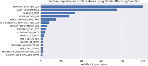
Meanwhile, in order to have a true predictive model of this research, we use the Gradient Boosting Classifier⁷ to classify the strongest feature parameter associated with the recent residual. Thus, we calculate the basic regression coefficient of the residual on the selected feature and then sum it together with the current coefficient for that variable. Figure 1 shows the variable RUNNING_TIME_PER_DAY of the generator is the key important feature which has a great influence on the output. This is followed by the DAILY_CONSUMPTION and the least feature importance parameter is GENERAL_1_CAPACITY_(KVA).

Figure 1. Feature importance ranking fitted using Gradient Boosting classifier.

Descriptive Statistics

Figure 2 displays that the fuel consumed by the generator has a skew value of $0.67$ and a kurtosis (the measure of distribution curve) of $0.40$ (refer to the left plot). The Gaussianity test in the right plot shows that there are some anomalies in the fuel consumed. This is clearly confirmed in Figure 3(left) where the generator working hours exceeded $24$ hours in a day. All these features are highly captured with the Gradient Boosting Classifier. The plot also reported that the average fuel consumed in a day is $\sim 262\mathrm{L}$. In effect, out of an observation size of $5905$, $35.11\mathrm{\%}$ is detected as an anomaly and this is clearly depicted in Figure 3 (right).

Figure 2. The distribution of fuel consumption. LEFT: A histogram showing the fuel consumed is slightly positively skewed. RIGHT: A probability plot showing that the fuel consumed is $\sim 96.29\mathrm{\%}$ Gaussian.

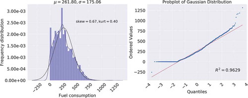
Figure 3. Graph of number of hours the generator function in 1 day (left) and pie chart of the target class labels (right).

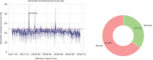
The pie chart in Figure 3 (right) shows that there is a class imbalance in the model data and this can affect the classification base task. This class imbalance is where the number of one class is significantly large compared to the other class. The effect of this would later be seen when we discuss about the performance measure in Section 5.

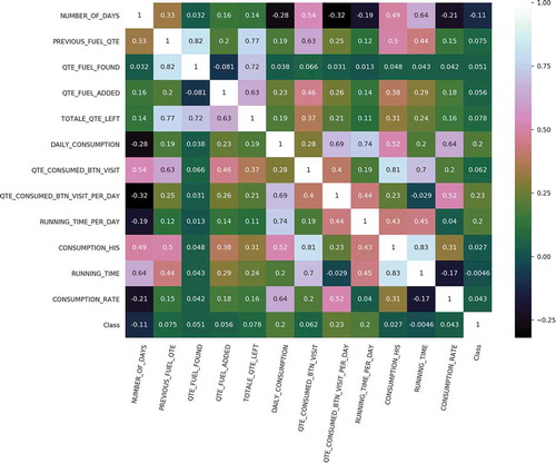
Figure 4 is a correlation matrix displaying the correlation coefficients between the feature parameters in Table 1. Correlation is a normalized covariance with its values ranging from $-1$ to $1$. The matrix measures a linear relationship between variables with $-1$ indicating that the related variables have a strong negative relationship, that is, as one variable increases, the other one decreases and $1$ indicates strong positive relation, that is, an increase in one variable results to increase in the other one. The diagonal values indicate the correlation of a variable with itself (known as auto-correlation). For instance, it can be seen from Figure 4 that the fuel consumed has a strong positive relation of $0.83$ with the number of hours the generator is working. This means that as the generator continues to operate for long hours, the fuel consumption directly increases.

Figure 4. A Correlation matrix measuring the linear dependence between the feature parameters.

The anomalies (also known as outliers) detected in the data include hours the generator was working in 1 day, consumption exceeding what the fuel generator can consume in a day and the case where the fuel consumed and running time are zero. These outliers were used to generate the classification class. In our case, these selected samples are defined as anomaly and the others (refer to Table 1) as normal.

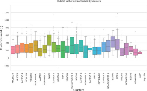
Figure 5 shows box plots of the fuel consumed by the clusters (also known as base stations). For the purpose of this study, the cluster is a group of sites where generators are located and therefore, the fuel consumed by a cluster is the total fuel consumed by different generators in the various sites. Note how most of the base stations have recorded outliers (thus, the dotted points on or below the whiskers) in the fuel consumption. In addition, Agip is the station that recorded the least of fuel consumption ($\sim 100\mathrm{L}$) in a day. On the average, most of the sites such as Kousseri, Guider, Ngaoundal, Waza, etc., consumed $\text{gsim}$ of fuel per day.

Figure 5. Fuel consumed per cluster.

Methods

Support Vector Machine

Support vector classifier is a supervised machine learning technique used to separate two or more classes by finding a hyperplane which maximizes the margin between them. In the case of linearly separable classes, an ideal hyperplane (decision plane) called decision boundary is defined to separate two classes with the widest margin that ensures the distance between the boundary of the two or more classes is maximized (Hastie, 2005). Given a pair of input variables $x\in R$ and corresponding class $d_i$ such that $d_i\in \{1,-1\}$, the classifier find a function that correctly maps each input variable $x_i$ to its corresponding class $d_i$. The decision boundary is defined as;

(1) $f(X)={\mathbf{W}}^{T}X+b$(1)

where $\mathbf{W}$ is the weight vector and $b$ the bias. The support vectors that is, the samples on the boundary of the margin determines the decision boundaries. If $f(X)$ in Equation 1 is greater than zero then the input variable belongs to class $1$, otherwise, it belongs to class $0$. To obtain an ideal hyperplane between the two classes, is the same as minimizing the norm of the weight vector (Hastie, 2005). For two-class classification, the input variable is either on the positive or negative side of the decision variable such that;

(2) $d_i({\mathbf{W}}^T{x}_i+b)\ge 1,\mathrm{\forall }(x_i,d_i),d_i\in \{-1,1\}$(2)

The margin can be maximized by minimizing the weight vector $\mathbf{W}$. In the case of non-separable, penalizing term is introduced to allow misclassification. The slack variable introduced in the case of non-separability measures how far the data deviate from the correct class (Kelleher, Namee, and D’arcy 2015).

(3) $d_i({\mathbf{W}}^T{x}_i+b)\ge 1-{\xi }_i,i=1\cdots N,0\le {\xi }_i\le 1$(3)

When a sample is correctly classified then the slack variable corresponding to that input value is equal to zero. For non-linear classes, the kernel functions transform the input example to a more separable space. A non-linear kernel function transforms the inputs to a more separable space and defines a hyperplane that clearly separates the classes. Commonly used non-linear function includes the hyperbolic tangent, polynomial and radial basic kernel (Aggarwal 2014).

Multilayer Perceptron

MLP is a supervised machine learning neural network inspired by the human brain (Haykin 1994). The classifier consists of input layer, hidden layers, activation function and output layer. The input layer receives the vector $X=\left[x_0,x_1,\cdots x_n\right]$ and assigns a weight vector $w=\left[w_0,w_1,\cdots w_n\right]$. MLP is a forward feed, that is, weighted input table:Variables move from the input layer to the inner hidden layer (Aggarwal 2014). The hidden layers enhance the model capabilities by allowing the network to learn complex problem and give result in the output layer. A nonlinear activation function applied to the weighted linear summation of the input table:Variables to extract a relationship between the output and input variable.

(4) $z=\sum _{i=1}^m{w}_{ji}{x}_i,$(4)

(5) $y=\varphi (z)$(5)

where $w_{ji}$ is the synaptic weight connecting neurons between the layers and $\varphi$ is the activation function which transforms the weighted sum of the input. The weight vector is unknown, therefore, weights in the input layer are randomly initialized based on the feature importance of the input variables. Hidden layers and activation function allow the model to learn non-linear function as a result, low weight value at the input layer allows the model to start as linear and due to increasing hidden layers, the model turns nonlinear with increased weights.

Commonly used nonlinear function is the sigmoid function. The weight adjustment is with respect to the error, that is, computed at each neuron to make sure error minimization. As a result of these connections, each node is penalized as every node contributes to the global error computed at the output layer. The aim is to minimize the error, therefore the error correction with respect to the weight (Haykin 1994) is done using the Gradient descent method and this is given as;

(6) $\mathrm{\Delta }{w}_{ji}^t=-\eta \frac{\mathrm{\partial }\epsilon (n)}{\mathrm{\partial }{w}_{ji}}$(6)

where $\eta$ is the learning rate and $\epsilon (n)$ is the error term. At the output node, the network error is computed. Noting that weights in the hidden layers are updated based on the error computed at the output node. Learning rate regulates the change of the adjusted weight in the direction of weight. A small value of $\eta$ controls the step size toward convergence whereas high value will cause divergence. To ensure the error is minimized, weights are adjusted such that the new weight became;

(7) $w_{kj}^{t+1}=w_{ji}^t-\eta \frac{\mathrm{\partial }\epsilon (n)}{\mathrm{\partial }{w}_{ji}}$(7)

The weight updates are done either in a batch, that is, using batch or the stochastic gradient descent methods.

K-Nearest Neighbors

KNN is a sluggish learning algorithm that depends on the knowledge gained from the training data to predict the test data. In general, the algorithm does not make any assumptions about the data but mainly bases its prediction on the $k$ neighboring terms. Therefore, if we consider to predict for unknown parameter, the KNN scheme will scan through the training data to obtain all the related instances that are close to the unknown points. For quantitative data, the Euclidean formula defined in Equation 8 is used to select the similarity points whilst for other data types like nominal or ordinal, Hamming distance can be applied.

(8) $D=||x_j-x_0||$(8)

Furthermore, in regression analysis, we measure the expectation of the predicted feature and for classification problems like in our case, the most dominant class is returned.

Since KNN depends on the number of $k$ neighbors during its testing phase and the algorithm uses distance measure to determine test class, the algorithm suffers from high computation cost. The choice of the value $k$ influences the performance of the model. A small value of $k$ can result in high accuracy but can results in over-fitting the model whereas for a large value of $k$, although the effect of noise is reduced, KNN is prompt to have lose boundary hence under-fitting the model.

Logistic Regression

LR makes use of conditional probability to map the input variable to a corresponding classification class. Given an input variable, the model predicts the probability of an input variable to belong to classification class. Suppose given an input variable $\mathbf{x}$ such that $\mathbf{x}=\left[x_0,x_1,\cdots x_n\right]$, and the corresponding class $y_i,\mathrm{\forall }i=1,\cdots ,p$ where $p$ represents the number of classes. LR uses non-linear activation, that is, the sigmoid function to give the relation between the input variables and the output class. In the case of binary classification where $y\in \{0,1\}$ is the probability of being in either class $0$ or $1$ is given by;

(9) $p(\mathbf{y}|\mathbf{x})=\frac{1}{1+e^{-\mathbf{z}}},\mathbf{z}=w_0+\sum _{i=1}^n{\mathbf{W}}^T\mathbf{x}$(9)

In this work, we aim to optimize the weighted parameters $\mathbf{W}$ so that the classification error can be minimized. These parameters are either estimated by gradient ascent or stochastic gradient ascent methods (Pedregosa et al. 2011). The log-likelihood and Newton methods are commonly applied to glean optimal parameters (Qi and Sun 1993). In both gradient cases, the hyperparameters are adjusted until the model has a minimum error between the observed value and the predicted. Here, the stochastic gradient ascent updates the weight at every single point depending on the direction of the weight. This distinguishes the two gradient cases.

Performance Evaluation

To evaluate the predictive capabilities of the fitted models, we adopt methods such as train-test split and K-fold cross validation methods. In this work, we evaluate our predicted models discussed in Section 3 using cross tabulation presented in Table 2. Here, the table presents a binary classification confusion matrix. From Table 2, the following information about the classifiers’ performances can be obtained as follows:

Table 2. Performance metrics for classification.

	Positive	Negative
Positive	True Positive (TP)	False Positive (FP)
Negative	False Negative (FN)	True Negative (TN)

• True positive (TP): correct prediction of positive class

• True negative (TN): predictions of negative class when the class is actually negative

• False negative (FN): wrong prediction of positive class as negative.

• False positive (FP): model predicts negative class predicted as positive.

Recall or sensitivity gives the classifier capability to correctly classify the positive class which is given as a ratio of TP and positive in the sample in the dataset. Other measures such as precision compare the true positive in the confusion matrix and the total number of positively predicted by the classifier. Specificity is also known as the true negative rate of the classifier, it is the ratio of true negative and negatives sample. F-measure the Harmonic mean of recall and precision. Equation 10 to 14 gives the formulae of the computation generated from the confusion matrix.

(10) $\mathrm{A}\mathrm{c}\mathrm{c}\mathrm{u}\mathrm{r}\mathrm{a}\mathrm{c}\mathrm{y}=\frac{\mathrm{T}\mathrm{P}+\mathrm{T}\mathrm{N}}{\mathrm{T}\mathrm{P}+\mathrm{F}\mathrm{P}+\mathrm{T}\mathrm{N}+\mathrm{F}\mathrm{N}}$(10)

(11) $\mathrm{R}\mathrm{e}\mathrm{c}\mathrm{a}\mathrm{l}\mathrm{l}(\mathrm{S}\mathrm{e}\mathrm{n}\mathrm{s}\mathrm{i}\mathrm{t}\mathrm{i}\mathrm{v}\mathrm{i}\mathrm{t}\mathrm{y})=\frac{\mathrm{T}\mathrm{P}}{\mathrm{T}\mathrm{P}+\mathrm{F}\mathrm{N}}$(11)

(12) $\mathrm{P}\mathrm{r}\mathrm{e}\mathrm{c}\mathrm{i}\mathrm{s}\mathrm{i}\mathrm{o}\mathrm{n}=\frac{\mathrm{T}\mathrm{P}}{\mathrm{T}\mathrm{P}+\mathrm{F}\mathrm{P}}$(12)

(13) $\mathrm{F}-\mathrm{m}\mathrm{e}\mathrm{a}\mathrm{s}\mathrm{u}\mathrm{r}\mathrm{e}=2\frac{\mathrm{P}\mathrm{r}\mathrm{e}\mathrm{c}\mathrm{i}\mathrm{s}\mathrm{i}\mathrm{o}\mathrm{n}\ast \mathrm{R}\mathrm{e}\mathrm{c}\mathrm{a}\mathrm{l}\mathrm{l}}{\mathrm{P}\mathrm{r}\mathrm{e}\mathrm{c}\mathrm{i}\mathrm{s}\mathrm{i}\mathrm{o}\mathrm{n}+\mathrm{R}\mathrm{e}\mathrm{c}\mathrm{a}\mathrm{l}\mathrm{l}}.$(13)

(14) $\mathrm{S}\mathrm{p}\mathrm{e}\mathrm{c}\mathrm{i}\mathrm{f}\mathrm{i}\mathrm{c}\mathrm{i}\mathrm{t}\mathrm{y}(\mathrm{T}\mathrm{N}\mathrm{R})=\frac{\mathrm{T}\mathrm{N}}{\mathrm{T}\mathrm{N}+\mathrm{F}\mathrm{P}}$(14)

Cross validation is a technique used to check how the model will perform in general. We performed K-fold cross-validation with $10$ folds. The data are split into K folds, that is, for $10$ folds, $9$ folds are used to train the data and the ${10}^{\mathrm{t}h}$ fold is used for testing. This process is repeated until all the folds are trained and tested. The accuracy of the classifier is obtained by taking the average of all accuracies gleaned in the test fold.

Due to the imbalanced nature of the normal and anomaly class in our dataset, ROC⁸ curves are used to measure how the classifier is performing in each class. As we saw earlier, the data is skewed and therefore, class distribution might affect classifier performance. The area under the curve (AUC) visualizes the classifier behavior on how often the model will classify positive class correctly and when the actual classification is negative, how often the model predicts positive. In this study, we want to maximize the true positive rate and minimize the false positive rate. The curve has TPR on the vertical axis and FPR on the horizontal axis. The plot ranges from $0-1$ with position (0,1) indicating a perfect classification model. The TPR and the FPR of the classifier is given by;

(15) $\mathrm{T}\mathrm{P}\mathrm{R}=\frac{\mathrm{T}\mathrm{P}}{\mathrm{T}\mathrm{P}+\mathrm{F}\mathrm{N}}$(15)

(16) $\mathrm{F}\mathrm{P}\mathrm{R}=\frac{\mathrm{F}\mathrm{P}}{\mathrm{F}\mathrm{P}+\mathrm{T}\mathrm{N}}$(16)

Results and Analysis

After accomplishing the normal feature engineering, selection, and as expected, fitting a classifier and obtaining some results in a form of a probability or a class, the next thing we need to do is to evaluate how efficient the classifier is on the metric performance using the validation dataset. In this work, the classification technique is done by splitting⁹ the model data into 80–20 ratio, to obtain the train and test sets, respectively.

Tables 3 and 4 show the performance of the fitted models (SVM, MLP, KNN and LR) on the dataset. For instance, in Table 3, the TPs are $752$ (for SVM), $773$ (for MLP), $696$ (for KNN) and $741$ (for LR). In the case of TNs, we have $369$ (SVM), $362$ (MLP), $310$ (KNN) and $95$ (LR). The lowest FP is recorded by MLP as $9$ and the highest is captured by KNN as $86$. A summary probability of these performances are reported in Table 4. For example, the MLP classifier recorded the highest score of $\sim 96.1\mathrm{\%}$ on the test data. This is followed by the SVM classifier which gave an accuracy score of $94.9\mathrm{\%}$ on the validated data. Moreover, the proportion of the dataset that is classified as an anomaly and actually detected as an anomaly in the positive class [refer to Equation 12] is $\sim 94.3\mathrm{\%}$ (for LR), $\sim 96.2\mathrm{\%}$ (for SVM), $\sim 89.0\mathrm{\%}$ (for KNN) and $\sim 98.8\mathrm{\%}$ (for MLP). Note also that, the model classifier that recorded the highest specificity is the MLP with a percentage value of $\sim 97.6\mathrm{\%}$.

Table 3. Classifier confusion matrix.

	Confusion matrix
	SVM	MLP	KNN	LR
TP	752	773	696	741
FP	30	9	86	41
TN	369	362	310	95
FN	30	37	89	304

Table 4. Classifier evaluation performance.

	Classification performance
Classifier	Accuracy	F1-Measure	Recall	Precision	Specificity
LR	0.708	0.811	0.709	0.943	0.699
SVM	0.949	0.962	0.962	0.962	0.925
KNN	0.851	0.888	0.887	0.890	0.783
MLP	0.961	0.971	0.954	0.988	0.976

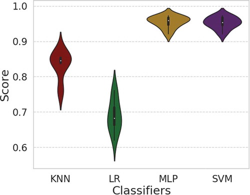
The Violin plots displayed in Figure 6 compare the 10-fold cross validation scores of the model classifiers. The white dot in the middle of the Violin plots denotes the median of each classifier. The thick gray bar in the center denotes the inter-quartile range whilst the thin gray line represents the $95\mathrm{\%}$ confidence interval. The colored regions (red, green, yellow and magenta) on each side of the gray line is a kernel density estimation depicting the distribution shape of the model data. Note how the MLP and SVM classifiers have broader regions around their respective medians. This clearly means that, these classifiers (MLP and SVM) have a higher probability scores than the other two classifiers (LR and KNN).

Figure 6. Violin plots showing the 10-fold cross validation score for LR, KNN, MLP, and SVM.

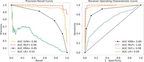
Figure 7 shows the ROC (right panel) and precision-recall (left panel) curves. Due to huge class imbalance in the dataset (refer to Figure 3) (right), the precision-recall curves is approximate for this study. Here, the MLP classifier registered an AUC of $99\mathrm{\%}$ followed by the SVM with an AUC of $96\mathrm{\%}$. These high values show that there is a trade-off between the true positive rate and the positive predictive value for these two classifiers, as relatively compared to KNN and LR. However, if we ignore the fact that there is a class imbalance in the dataset, then we measure the agreement between the true positive rate and false-positive rate for the predictive model. In this case, we consider the right panel curves. Note how the ROC curves overestimated the probabilities of the model classifiers. This is clearly due to the huge skewness in the distribution of the sample data. Hence, for the purpose of this study, we choose the left panel curves as appropriate.

Figure 7. Precision-Recall curves and ROC curves of classifiers.

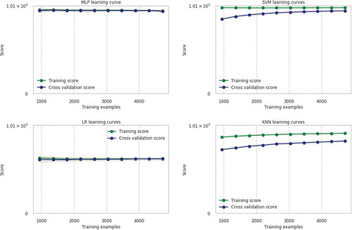
Using cross validation with 10 splits, we can observe the relationship between training score and cross validation score of different classifiers as presented in Figure 8. The variation of cross validation curve results in high variance and that of the training score curve results in high bias. High variance is an indication that the model detects every noise in the data. High bias implies that the model data has less information. Regularization of bias and variance help the model to attain better predictive performance. The graphs presented in Figure 8 show that the cross validation curve tends to converge with increase in the training sample. In this work, the MLP and LR converge just after $1000$ training samples whilst the other two classifiers slowly converge and may require more training samples that is $>5000$.

Figure 8. Training and cross validation score curve of MLP, KNN, SVM, and LR.

Conclusion

In this paper, we aimed at evaluating the classification algorithm by training the model to learn and identify the anomalies in the fuel consumption dataset obtained from a telecommunication base station. Four classification techniques were evaluated namely; SVM, LR, MLP, and KNN. MLP recorded the best performance generally with an accuracy score of $96.1\mathrm{\%}$ on the test data. Although the SVM outperformed the other two classifiers (KNN and LR), using the K-fold cross validation technique, the MLP again slightly performed better than SVM with a score of $96.1\mathrm{\%}$. Furthermore, from the performance measure table, the MLP registered the best predicting power of detecting the anomalies. The LR also performed better than the KNN in the precision score with respective values of $96.1\mathrm{\%}$ and $89.0\mathrm{\%}$. The class imbalance in the dataset resulted in the work to choose the Precision-recall curve over the ROC curve to avoid overestimation. Again, the MLP recorded an AUC of $99.0\mathrm{\%}$ as the highest performance classifier. This is followed by SVM with an AUC of $96.0\mathrm{\%}$. We therefore conclude that the MLP classifier gives the overall best performance over the other classifiers, that is, the classifier best fits the training examples compared to other classifiers in terms of anomaly detection and in evaluation performance such as K-fold cross validation as well as the use of the precision-recall curves.

Acknowledgements

The author would like to thank TeleInfra Company and Group One Holding Company for providing the dataset for this study. We wish to acknowledge Mr. OKALI DIMA Patrick from Group one holding for ensuring the data were available. Grateful for SciKit learn library as this work has been made possible from the use of their library packages. T. Ansah-Narh is very grateful to the Data Science Intensive (DSI) Program, organised by the African Institute for Mathematical Sciences (AIMS) South Africa, in conjunction with SA-DISCNet.

Notes

1. http://www.art.cm/en/node/3111.

2. Support Vector Machine.

3. K-Nearest neighbors.

4. Logistic Regression.

5. MultiLayer Perceptron.

6. Here, the NaN values are removed using the Pandas module dropna.

7. Using the Python module sklearn.ensemble.GradientBoostingClassifier, we can compute the feature import to choose the relevant feature parameters. Note, this classifier uses the forward stagewise algorithm.

8. Receiver Operating Characteristic.

9. Here, we separate the dataset into train and test sets using the Python SciKit module sklearn.model_selection.train_test_split.

References

- Aggarwal, C. C. 2014. Data classification: Algorithms and applications. Boca Raton, Florida, United States: CRC press.
- Banjanovic-Mehmedovic, L., A. Hajdarevic, M. Kantardzic, F. Mehmedovic, I. Dzananovic. 2017. Neural network-based data-driven modelling of anomaly detection in thermal power plant. Automatika. 58(1):69–79. doi:10.1080/00051144.2017.1343328.
- Chouiekh, A., and I. E. L. H. EL Hassane. 2018. Convnets for fraud detection analysis. Procedia Computer Science 127:133–38. doi:10.1016/j.procs.2018.01.107.
- Hastie, T., Tibshirani, R., Friedman, J., and Franklin, J. 2005. The elements of statistical learning: data mining, inference and prediction. The Mathematical Intelligencer 27(2):83-85. Springer. doi:10.1007/BF02985802.
- Haykin, S. 1994. Neural networks: A comprehensive foundation. Upper Saddle River, New Jersey, United States: Prentice Hall PTR.
- Kelleher, J. D., B. M. Namee, and A. D’arcy. 2015. Fundamentals of machine learning for predictive data analytics: Algorithms, worked examples, and case studies. Cambridge, Massachusetts, United States: MIT Press.
- Pedregosa, F., Varoquaux, G., Gramfort, A., Michel, V., Thirion, B., Grisel, O., Blondel, M., Prettenhofer, P., Weiss, R., Dubourg, V., et al. 2011. Scikit-learn: Machine learning in Python. Journal of Machine Learning Research 12 Oct: 2825–30.
- Qi, L., and J. Sun. 1993. A nonsmooth version of Newton’s method. Mathematical Programming 58 (1–3):353–67. doi:10.1007/BF01581275.
- Taboada-Crispi, A., Sahli, H., Hernandez-Pacheco, D., Falcon-Ruiz, A. 2009. Anomaly detection in medical image analysis. In Handbook of research on advanced techniques in diagnostic imaging and biomedical applications, 426–46. Pennsylvania, United States: IGI Global.
- Zanin, M., M. Romance, S. Moral, R. Criado, et al. 2018. Credit card fraud detection through parenclitic network analysis. Complexity 2018. Hindawi. doi:10.1155/2018/5764370.