CNN-VSR: A Deep Learning Architecture with Validation-Based Stopping Rule for Time Series Classication

ABSTRACT

Deep learning methods for univariate time series classification (TSC) are recently gaining attention. Especially, convolutional neural network (CNN) is utilized to solve the problem of predicting class labels of time series obtained through various important applications, such as engineering, biomedical, and finance. In this work, a novel CNN model is proposed with validation-based stopping rule (VSR) named as CNN-VSR, for univariate TSC using 2-D convolution operation, inspired by image processing properties. For this, first, we develop a novel 2-D transformation approach to convert 1-D time series of any length to 2-D matrix automatically without any manual preprocessing. The transformed time series will be given as an input to the proposed architecture. Further, the implicit and explicit regularization is applied, as time series signal is highly chaotic and prone to over-fitting with learning. Specifically, we define a VSR, which provides a set of parameters associated with a low validation set loss. Moreover, we also conduct a comparative empirical performance evaluation of the proposed CNN-VSR with the best available methods for individual benchmark datasets whose information are provided in a repository maintained by UCR and UEA. Our results reveal that proposed CNN-VSR advances the baseline methods by achieving higher performance accuracy. In addition, we demonstrate that the stopping rule considerably contributes to the classifying performance of the proposed CNN-VSR architecture. Furthermore, we also discuss the optimal model selection and study the effects of different factors on the performance of the proposed CNN-VSR.

Introduction

Time series data can be obtained from everywhere in everyday life. It is constantly generated from various human activities and different real world applications, such as biomedical signals, weather recordings, stock exchange rates, and many more. The time series analysis tasks mainly involve trend fitting, forecasting, clustering, and classification. In particular, in this article, we focus on the classification of time series. The time series classification (TSC) (Xing, Pei, and Keogh 2010) have many potential applications in the areas like healthcare (Wiens, Horvitz, and Guttag 2012), finance (Delgado, Cuellar, and Pegalajar 2008), engineering (Chen et al. 2014) and entertainment (Esling and Agon 2013). As univariate time series is the simplest type of time series data, this provides a reasonably good beginning point to analyze such temporal signals. A univariate TSC problem can be defined as, $t{s}_n\to c{l}_c$ so that $n$ number of time series of length $l:t{s}_n=\left(t{s}_{1_l},t{s}_{2_l},...,t{s}_{n_l}\right)$ can be associated with $c$ number of class labels $c{l}_c\in \{c{l}_1,c{l}_2,\cdots ,c{l}_c\}$. An application example of univariate TSC is to identify different heartbeats in electrocardiography data for monitoring the heart activities (Acharya et al. 2017). Moreover, it is also used in identifying household appliance working at a particular time frame (Lines et al. 2011).

The TSC problem has been explored and different types of TSC methods have been proposed in the past few decades due to its wide applicability and increase in time series datasets in various real world domains. The existing methods for TSC can be grouped from different perceptions. On the basis of feature types, it can be categorized as time domain or frequency domain methods. Time domain includes autoregression, cross-correlation, and autocorrelation analysis, while latter one includes wavelet and spectral analysis. It can also be categorized on the basis of strategy used for classification as distance-based methods, feature-based methods and model-based methods. The distance-based methods serve as earliest baseline, which work with raw time series. These methods measured similarity between any two given time series with some pre-defined similarity metrics such as dynamic time warping (DTW) (Li 2015) or Euclidean distance. Based on these similarity measures, the classification can be performed by applying algorithms such as k-nearest neighbors (k-NN). The combination of k-NN and DTW is a very efficient classifier, and it is known as a golden standard for TSC in last decade (Kate 2016) (Rakthanmanon et al. 2013; Jeong, Jeong, and Omitaomu 2011). For feature-based methods, a set of features are extracted for given time series that help in representation of patterns in data. Usually, after quantization, these patterns are represented in the form of bag of words, then fed to the classifiers (Lin et al. 2007). To name some recent benchmarks, bag of features framework (TSBF) (Baydogan, Runger, and Tuv 2013), bag of symbolic Fourier approximation symbols (BOSS) (Schäfer 2015) and BOSS with vector space model (BOSSVS) (Schäfer 2016) are used to extract features. The final classification is done using 1-NN classifier. Moreover, the model-based methods assume that a particular class sequence generated by an underlying model and parameters of the model are determined and fitted by the training set in the class. The simplest proposed model is Naive Bayes sequence classifier (Lewis 1998). However, the assumption of independence among features of different classes often violates for real life problems. The hidden Markov model is able to model the dependency between features of different classes and recently applied to TSC (Antonucci et al. 2015). Further, some ensemble approaches have been proposed for TSC, which combine multiple classifiers together to achieve better accuracy. From all ensemble approaches, to the best authors’ knowledge, the flat collective transform-based ensemble (COTE) provides better accuracy for time series datasets. It is a combination of 35 classifiers, which extract features from both frequency and time domain.

All the above-discussed methods require heavy crafting for pre-processing of data and extraction of features from time series signals. There are also some complexities associated with all of the methods. For distance-based methods, the length of given two time series must be equal and it is also sensitive to volatile nature of real time series data. Although, DTW has always been popular for time series data mining tasks but is computationally expensive and unable to satisfy the triangle inequality. For all the feature-based methods, the performance of classifier highly depends on the designing of features. It is to note that the application of the model-based approaches are limited by the fact that generally the time series obtained from real applications cannot, or very tough to be represented by a generative model.

In recent years, learning through deep neural network has achieved great recognition in fields like speech recognition and computer vision. Convolutional neural network (CNN) becomes one of the most popular among all deep learning architectures. Unlike the conventional feature-based classification methods, CNN does not need hand-crafted features. Both feature extraction and classification parts are unified in one model and are learned jointly. Moreover, CNN produced very impressive results in the field of image and signal processing for face identification, object recognition and masking (Schmidhuber 2015; Bengio, Courville, and Vincent 2013; Längkvist, Karlsson, and Loutfi 2014; Bengio 2013). Further, CNN has also been explored to few non-computer vision domains (Sak, Senior, and Beaufays 2014; Sezer and Ozbayoglu 2018; Ijjina and Mohan 2016; Costa, Oliveira, and Silla 2017). The main reason behind the success of CNN is its capability to learn complex features automatically using its multiple layers. Furthermore, there have been some research efforts in the area of TSC to exploit the abilities of deep learning, especially CNN. In Zheng et al. (2016), the authors proposed a multi channel CNN for multivariate TSC. A sliding window method is applied to enhance the time series data, and the results are presented with only two multivariate datasets and no experiments are performed on benchmark datasets. In Cui, Chen, and Chen (2016), a multi scale CNN approach is proposed for univariate TSC. The authors manually pre-process data for multi-scale settings using skip sampling, down sampling, and sliding window operation. However, due to large set of hyper-parameters and heavy preprocessing, it is difficult to deploy method presented in Cui, Chen, and Chen (2016). In Wang, Yan, and Oates (2017), the authors proposed three frameworks namely multi-layer perceptron (MLP), residual network and fully convolutional network. Their deep architectures perform well on small datasets but still prone to over-fitting. Both Cui, Chen, and Chen (2016) and Wang, Yan, and Oates (2017) provided comparative results on University of California Riverside (UCR) benchmark datasets (Chen et al. 2016). Further, the authors in Zhao et al. (2017) have proposed a shallow network architecture, however, the methods require hyper-parameters fine tuning, which can be tedious tasks in application to different datasets. Moreover, deep networks may be prone to over-fitting and unwanted chaotic behavior and therefore require additional computational cost. There is also a possibility that a shallow network may not be capable to uncover the dynamic behavior of the data.

Motivated by the CNN for image processing applications, we explore deep learning for TSC problem. In this study, we propose a novel CNN model with validation-based stopping rule (VSR) named as CNN-VSR for univariate TSC using two dimensional(2-D) convolution operation. For this, first we develop a novel approach that can transform any one dimensional (1-D) time series signals to 2-D matrices without any manual preprocessing. In order to transform the any time series signal of length $l$, we find out the optimum number of row $r$ and columns $c$ using simple factorization method. This method can be easily generalized to any time series data obtained from different real world problems. To the best of our knowledge, this simple 2-D transformation method is novel approach to convert the 1-D signal to 2-D matrices automatically without any manual pre-processing. The transformed time series will be given as an input to the proposed architecture. Thereafter, we propose a novel CNN architecture with VSR (CNN-VSR) for univariate TSC problem. Here, we introduce the stopping rule to avoid over-fitting, which is simple to apply with any CNN architecture (Prechelt 2012). Moreover, convolution and pooling operations are applied alternatively to extract deep features of the transformed time series data. Thereafter, the extracted features are fed to an MLP as an input to perform classification. In contrast to Cui, Chen, and Chen (2016), Wang, Yan, and Oates (2017) and Zhao et al. (2017), where the performance has been compared with limited number of straw-man methods, in this article, we compare the performance of proposed CNN-VSR architecture with the best available state of art method for individual datasets whose information are provided in the comprehensive repository for TSC maintained by UCR and University of East Anglia (UEA). Our results reveal that the proposed CNN-VSR architecture actually performs remarkably well.

Moreover, subtle fine tuning is needed with CNN architectures to boost the performance of classifier (Uktveris and Jusas 2017; Gurcan et al. 2002). This involves selecting an optimal model of CNN, which includes selection of a architecture and parameter settings. Therefore, these nuances and their effect on performance of classification are well investigated and discussed in this article. Further, it is important to note that, we did not require extensive hyper-parameter tuning as the objective function has been optimized using adaptive gradient descent. This gradient method have per-parameter learning rate, which applies heuristic approach without the need of heavy manual work in tuning hyper-parameters for learning rate schedule.

The structure of the rest of article is organized as follows. Section 2 presents the details of CNN-VSR approach. In Section 3, the experimental setup to evaluate the performance of proposed approach is presented. Section 4 provides the empirical analysis and demonstrates effectiveness of CNN-VSR approach in detail. Finally, the conclusion is presented in Section 5.

The Methodology

In this section, we present a novel CNN architecture to classify the univariate time series data. For this as inspired by image processing properties, we develop a novel 2-D transformation approach to convert 1-D time series of any length to 2-D matrix automatically. The transformed time series will be given as an input to the proposed architecture. Thereafter, we present a novel CNN-VSR architecture. Further, the early stopping rule for the proposed architecture is discussed. Moreover, for fine-tuning of the proposed architecture, we also discuss the optimal architecture and parameter settings.

Transformation of Time Series

Success of traditional CNN for image classification is well known. To utilize the capability of traditional CNN, we transform the 1-D time series signals into 2-D matrices. Therefore, a linear transformation of 1-D (univariate) time series to 2-D matrix is defined (see Figure 1 at the next page). Before transforming a time series, each time series is normalized using centering and whitening process. This is required to compare time series with different amplitudes and offsets (Keogh and Kasetty 2003). Therefore, a time series of length $l$ can be converted into 2-D matrix of row $r$ and column $c$ such that it satisfies the condition $l=r\times c$. Let $l$ is assumed as the product of prime numbers $P$, then the set of prime numbers is divided into two subsets $S_1$ and $S_2$, such that the difference of the sum of members of subsets is minimized. Hence, $r$ and $c$ are the product of the members of subsets $S_1$ and $S_2$, respectively. The term $l,P,r$, and $c$ are mathematically defined as

(1) $l=\prod _{i=1}^n{P}_i,$(1)

(2) $P=S_1\bigcap S_2:\mathrm{m}\mathrm{i}\mathrm{n}\mathrm{i}\mathrm{m}\mathrm{i}\mathrm{z}\mathrm{e}\mathrm{d}\left|\left(\sum S_1\right)-\left(\sum S_2\right)\right|,$(2)

(3) $r=\prod _{i=1}^m{S}_{1i},c=\prod _{i=1}^n{S}_{2i}.$(3)

Algorithm 1 Transformation of training set

1: Let l be the length of time series of a training set and ts is the time series

2: procedure Transform($l,ts$)

3:  p = 2, k = 1, i = 0

4:  while $l\ge p^2$ do

5:   if $lmodp==0$ then

6:    store p into an array pri[]

7:    $l=l/p$

8:   else $p=p+1$

9:   end if

10:  end while

11:  $n=sizeofpri[]$

12:  $\mathrm{C}\mathrm{a}\mathrm{l}\mathrm{l}\mathrm{p}\mathrm{r}\mathrm{o}\mathrm{c}\mathrm{e}\mathrm{d}\mathrm{u}\mathrm{r}\mathrm{e}\mathrm{D}\mathrm{I}\mathrm{M}(pri,n-1,0,0,1,1)$

13:  for each time series $ts$ in training set do

14:   for $i=1torow$ do

15:    for $j=1tocol$ do

16:     $trans[i][j]=ts[k]$

17:     $k=k+1$

18:    end for

19:   end for

20:  end for

21: end procedure

22: procedure dim $(pri[],n,s1,s2,r,c)$

23:  if $n<0$ then

24:   return $\left|s1-s2\right|$

25:  end if

26:  $m=\mathrm{D}\mathrm{I}\mathrm{M}(pri,n-1,s1+pri[n],s2,r\times pri[n],c)$

27:  $n=\mathrm{D}\mathrm{I}\mathrm{M}(pri,n-1,s1,s2+pri[n],r,c\times pri[n])$

28:  if $s1-s2==min(m,n)$ then

29:   $row=r\mathrm{a}\mathrm{n}\mathrm{d}col=c$

30:   $\mathrm{r}\mathrm{e}\mathrm{t}\mathrm{u}\mathrm{r}\mathrm{n}row\mathrm{a}\mathrm{n}\mathrm{d}col$

31:  end if

32: end procedure

Figure 1. Transformation of training set.

The transformed training set (see Figure 1) will be given as an input to the proposed architecture, which is proposed in the next section. Overall, the transformation of training set is summarized in the Algorithm 1.

The Proposed Architecture

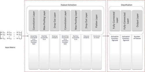
This Section presents the architecture of the proposed CNN model. It consists of multiple layers, which deal with feature extraction and classification of time series datasets. There are two convolutional layers, two max-pooling layers, two dropout layers, one flatten layer, and three fully connected layers (see Figure 2). The specific architecture has been finalized by testing multiple architectures (see Section 2.3.1). Every feature learning layers depict different feature-level, number of filters, activation function, and pooling operators. Each layer receives and produces feature maps as input and output respectively. Moreover, with the help of Eq. (2), the layers are convolved with kernel size of (3,3). The convolutional layer is the heart of any CNN model and reinforces a local connectivity pattern by utilizing spatially local correlation between neurons of adjoining layers. After each convolutional layer, feature maps are connected to max-pooling layer. The main reason for applying max-pooling function is to reduce the size of feature maps. Further, the parameters for neurons are obtained through brute force method and the filter size and stride of convolutional layer is set to 3 and 1, respectively. Furthermore, the Rectified Linear Unit (ReLU) and sigmoid activation function are used in our proposed model. The ReLU activation function is used in convolutional layers to capture interactions and non-linearities in time series data, whereas the sigmoid activation function is used in fully-connected layers to classify the features extracted from previous layers. The sigmoid activation function allows model to learn the complex structures. Finally, at the end of first stage, feature extracted are flattened and sent as an input to fully connected layers to classify the given time series. Fully-connected layers are similar to the traditional MLP as each neuron of one layer is connected to each neuron in another layer. The proposed pipeline of layers of CNN architecture for TSC is shown in Figure 2. The brief description of each layer used in proposed architecture is described below.

Figure 2. Architecture of proposed CNN model.

Convolution

Convolution is a mathematical construct, which is widely applicable in processing of digital signals. These signals are mostly represented in the form of time series. In layman’s terms, convolution can be defined as a method for combining or blending two functions of time in an adhesive form (Weisstein 1999). The 2-D convolution function with two input matrices having dimensions $I(ra,ca)$ and $K(rb,cb)$ can be mathematically described as

(4) $C(i,j)=\sum _{m=0}^{ra}\sum _{n=0}^{ca}I(m,n)K(i-m,j-n),$(4)

where $0\le i<ra+rb-1$ and $0\le j<ca+cb-1$.

Pooling

Pooling operation perform nonlinear down-sampling of the input. This operation divides the input signal into many non-overlapping rectangular regions. For each such region, it produces output as average or maximum value. This helps in reducing the feature size as requisite, and it also provides translation invariance. Moreover, a max-pooling operation computes the maximum value as an output, therefore, mathematically it can be written as

(5) $z_{ij}=\mathrm{m}\mathrm{a}\mathrm{x}\left\{z_{i\prime ,j\prime }:i\le i\prime <i+p,j\le j\prime <j+p\right\},$(5)

where $z$ is the output and $p$ is the padding.

Dropout

The idea of dropout in neural network is to dropout the units of both visible and hidden layers randomly. It can be viewed as a regularization approach to avoid over-fitting in the training phase. This operation diminishes complex co-adaptations among neurons. Therefore, it is helpful in learning more robust features. For implementation, a mask is created of zeros and ones during forward pass in training to deactivate neurons.

Flattening

The final stage of any CNN is a classifier. It is also referred as a dense layer, which is an artificial neural network classifier. The classifier requires a vector of individual features as an input. Therefore, it is needed to transform the output of feature extraction into 1-D feature vector. This mechanism is known as flattening.

Non-linear Gating

Non-linear filters of traditional CNN uses non-linear gating function with a linear functions, which is applied identically to every constituent of a feature map. The most used non-linear gating function is the ReLU function. Such filter can be mathematically expressed as

(6) $z_{ik}=\mathrm{m}\mathrm{a}\mathrm{x}\left\{0,x_{ik}\right\}.$(6)

where $x$ is the input and $z$ is the output.

Adaptive Stochastic Gradient Descent

Adaptive optimization is an extension to stochastic gradient descent algorithm. Unlike stochastic gradient, it maintains the learning rate for every network per-parameter and adapted distinguishably as learning continues from first and second moment computations. It is well suited for convex and non-convex problems for quick convergence (Kingma and Jimmy 2014). Mathematically, its update rule can be represented as

(7) ${\theta }_{t+1}={\theta }_t-\frac{\eta }{\sqrt{\widehat{v_t}}+\epsilon }\widehat{m_t},$(7)

where $\eta$ is the learning rate, $m_t$ is the first moment and $v_t$ is the second moment of the gradients.

Optimal Model Selection

Architecture Selection

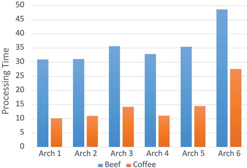
Choosing the best architecture provides greater probability of achieving better results in different neural network applications (Balkin and Keith Ord 2000). CNN supports sequentially connected layers. Due to different types of layers, it is not trivial to get an optimal sequence that closely suits to the given problem. Therefore, in this article, we model the layer selection process as a Markov Decision Process with the assumption that a well-performing layer in one network should also perform well in another network. We make this assumption based on the hierarchical nature of the feature representations learned by neural networks with many different layers (LeCun, Bengio, and Hinton 2015). Mostly, four layers are popular among researchers, which deal with TSC namely; convolutional layer, pooling layer, fully-connected layer (Dense layer), and ReLU layer. In addition, we have added dropout layer to suppress the over-fitting in the data. The multiple combinations of these layers are trained for chosen learning problem using benchmark datasets. In this article, we have tested six different CNN architectures. The configuration of architectures in a simplified notation is presented in Table 1. We selected the best-suited architecture on the basis of testing accuracy and processing time of algorithm. Therefore, architecture five (see Table 1 at the next page) is selected for our learning problem due to its better testing accuracy in comparison to other architectures (see Figure 3 at the next page), and it is also competitive with other architectures in terms of processing time (see Figure 4 at the next page).

Table 1. Notation for different architectures.

#	Architectures	Notations
Arch 1	ICMDoFDDDO	I = Input layer of size
Arch 2	ICMRDoFDO	C = Convolutional Layer
Arch 3	ICMCMODoFDDO	F = Flatten Layer
Arch 4	ICMDoCRFDDDO	Do = Dropout Layer, O = Output Layer
Arch 5	ICMDoCMDoFDDDO	D = Dense Layer, R = ReLU Layer
Arch 6	ICMCRDCMDoFDDO	M = Max-Pooling Layer

Figure 3. CNN architectures accuracy evaluation.

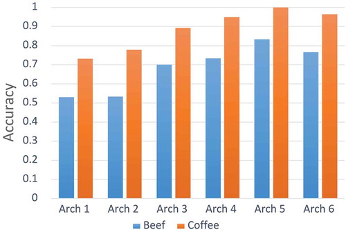
Figure 4. CNN architectures processing time evaluation.

Parameters Selection

Although deep learning has achieved promising results on many tasks, training and fine-tuning of a good model normally require significant efforts. This is because, several important parameters needed to be evaluated, such as learning rate, dropout ratio, and the number of training iterations. For instance, a small learning rate may demand much more iterations to converge, while a large value may accelerate the convergence but can possibly result in oscillation. In addition, a larger dropout ratio may lead to a better model but could probably slow down the convergence. There is no universal rule for parameter selection. With the goal of providing some insights on parameter selection especially for the problem of TSC, we study different sets of parameters using the aforementioned network architecture using benchmark datasets. The final sets of parameters are shown in Figure 2. These parameters have been finalized by reducing the cross-validation error of proposed CNN architecture (Anders and Korn 1999).

Learning

Learning of proposed CNN architecture is analogous to the training of any MLP. Each neuron in the MLP contains an activation function, which maps the weighted inputs to the output. An MLP is said to have a deep architecture when it contains more than one hidden layer. Similarly, a CNN referred as MLP with special architecture. Generally, CNN is composed of two steps. In first step, deep features of raw data are generated using convolution and pooling functions alternatively, whereas in Step 2, an MLP classifies the deep features generated in previous step. Moreover, there are two important aspects for designing any CNN, which are appropriate architecture and best learning algorithm. The learning algorithm and architecture should be compatible with each other and fit to the data appropriately.

Algorithm 2 Learning with VSR

1: let $\theta$ be the initial set of parameters and ${\theta }^{\prime }$ be the best parameters.

2: Let $n$ be the number of folds, $e$ is the number of epochs and $q$ is the patience.

3: procedure VSR($n,e,\alpha ,q$)

4:  $j=0,i=0,L_{lw}=\mathrm{\infty }$

5:  for $1tonfolds$ do

6:    while $j<e$ do

7:     update $\theta$ by running the training algorithm

8:     update $L_{lw}(e),L_{va}\left(e\right)$ using Eqs. (9) and (10)

9:     if $L_{gen}\left(j\right)>\alpha$ then using Eq. (11)

10:       ${\theta }^{\prime }=\theta \mathrm{s}\mathrm{a}\mathrm{v}\mathrm{e}\mathrm{t}\mathrm{h}\mathrm{e}\mathrm{b}\mathrm{e}\mathrm{s}\mathrm{t}\mathrm{p}\mathrm{a}\mathrm{r}\mathrm{a}\mathrm{m}\mathrm{e}\mathrm{t}\mathrm{e}\mathrm{r}\mathrm{s}$

11:       $j=j+1$

12:     else

13:      while $i\le q$ do

14:       if $L_{gen}\left(j\right)>\alpha$ then using Eq. (11)

15:        ${\theta }^{\prime }=\theta \mathrm{s}\mathrm{a}\mathrm{v}\mathrm{e}\mathrm{t}\mathrm{h}\mathrm{e}\mathrm{b}\mathrm{e}\mathrm{s}\mathrm{t}\mathrm{p}\mathrm{a}\mathrm{r}\mathrm{a}\mathrm{m}\mathrm{e}\mathrm{t}\mathrm{e}\mathrm{r}\mathrm{s}$

16:       else

17:        if $i==q$ then

18:         $\mathrm{B}\mathrm{r}\mathrm{e}\mathrm{a}\mathrm{k}(\mathrm{s}\mathrm{t}\mathrm{o}\mathrm{p}\mathrm{t}\mathrm{h}\mathrm{e}\mathrm{l}\mathrm{e}\mathrm{a}\mathrm{r}\mathrm{n}\mathrm{i}\mathrm{n}\mathrm{g}\mathrm{p}\mathrm{r}\mathrm{o}\mathrm{c}\mathrm{e}\mathrm{s}\mathrm{s})$

19:        else$i=i+1$

20:        end if

21:       end if

22:      end while

23:     end if

24:    end while

25:  end for

26:  use the best parameters ${\theta }^{\prime }$ to compute the testing accuracy

27: end procedure

Backpropagation training process is applied for estimation of the parameters of the model (LeCun et al. 1998) (LeCun et al. 2012). Each backpropagation training phase has four main sections, named as: forward pass, loss function, backward pass, and weight update. The goal of this phase is to train a model that provides accurate class predictions for new unlabeled time series data. To fulfil this purpose, we have used a training set $X=\{(t{s}_{1_l},c{l}_1),(t{s}_{2_l},c{l}_2),\cdots ,(t{s}_{n_l},c{l}_n)\}$ of labeled time series of finite length $l$. 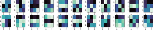In forward pass, we fed the transformed data (see Section III(A)) $X=\{((t{s}_{1_r}\times t{s}_{1_c}),c{l}_1),((t{s}_{2_r}\times t{s}_{2_c}),c{l}_2)$$,\cdots ,((t{s}_{n_r}\times t{s}_{n_c}),c{l}_n)\}$ as an input to pass it through the whole network architecture. Further, during forward pass, the feature maps are determined on input matrix by passing it from one layer to another layer until it reaches the output (from left to right in Figure 2). Moreover, the 22 feature maps obtained from convolutional layer has been presented for one benchmark dataset in the Figure 5. After that, the propagation error is estimated using loss function for the produced output (error propagates from right to left in Figure 2). Further, we have utilized cross-entropy as loss function (objective function) to compute error between targets and predictions. It can be described as

(8) $L_{ts}=-\sum t_{ts,cl}\mathrm{l}\mathrm{o}\mathrm{g}\left(p_{ts,cl}\right),$(8)

Figure 5. Visualization of 21 convolutional kernels of size 3$\times$3 learned by first convolution layer on the Synthetic Control benchmark time series data of input matrix of 10$\times$6.

where $t$ is the target, $p$ is the prediction, $ts$ represents the time series and $cl$ denotes the class label. Computed error on every layer is utilized for gradient (derivative) calculations to find out the direction to change parameters for convolutional and fully-connected layers, and accordingly the weights can be updated. Moreover, the non-linear gating function (see Section 2.2.5) can be adopted into the derivative by limiting the contributions from convolution kernels that have been turned off by the ReLU function. In this article, we have applied the adaptive stochastic gradient descent for optimization of the proposed model. The proposed network architecture is learned iteratively by backpropagation over a number of epochs, where one epoch can be defined as the interval during which each time series from the training set has been used once. In each epoch the training set is divided into mini-batches for batch-wise optimization. The learning rate for the batch-wise optimization is controlled by per-parameter adaptively using the Adam method based on the variance of the gradient. Parameters of Adam are chosen as recommended in (Kingma and Jimmy 2014). The mean loss over all time series samples during validation is calculated in evaluation phase after each epoch. The selected model used for the evaluation is the one, which achieves the lowest validation loss. To fulfil this objective, we required early stopping (Prechelt 2012) of learning and therefore, a VSR is described in next section.

Validation-Based Early Stopping Rule (VSR)

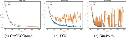
Although, when to stop learning has been always important question in training a supervised classifier, as it may lead to under-fitting or over-fitting of data. However, all traditional neural networks prone to over-fitting such as MLP (Geman, Bienenstock, and Doursat 1992). Generally, validation is applied to understand when over-fitting starts in supervised training set. Previously, plot of error in training and validation over time is utilized to find the optimum number of epochs (see Figure 6a at the next page), but this approach can not be generalized to Figure 6b,c, because the curves shown in these figures have more than one local or global minimum. Hence, it is impossible to determine from these curves that when to stop learning. Therefore, there is a requirement of better validation-based early stopping rule, which can be used to avoid over-fitting of data.

Figure 6. Training and validation loss curves.

Before describing stopping rule, some definitions are needed. Let $L$ be the objective function (loss function) used in the training algorithm, then $L_{tr}\left(e\right)$, the training set loss, is the average loss per example over the training set, measured after epoch $e$. Further, $L_{va}\left(e\right)$ is defined as validation loss, which is the corresponding loss on the validation set, and it is used in stopping rule. $L_{ts}\left(e\right)$, the test loss is the corresponding loss on the test set. $L_{ts}\left(e\right)$ is unknown during training process but it is assumed to use in estimation of generalization loss. In real life, the generalization loss is usually unknown, so that only the validation error can be used to estimate it. The $L_{lw}\left(e\right)$ is defined as lowest validation set loss and can be obtained in epochs upto $e$ as

(9) $L_{lw}(e)=\underset{e^{\prime }\le e}{\mathrm{m}\mathrm{i}\mathrm{n}}{L}_{va}(e^{\prime }).$(9)

Generalization loss is the relative increase of validation set loss obtained in epoch upto $e$ over the minimum value so far. It can be defined as

(10) $L_{gen}\left(e\right)=100\left(\frac{L_{va}\left(e\right)}{L_{lw}\left(e\right)}-1\right).$(10)

Moreover, the training will be stopped as soon as the $L_{gen}\left(e\right)$ stops showing any improvement. In other words, when the $L_{gen}\left(e\right)$ falls below the certain threshold $\alpha$ the training will be stopped. Mathematically, it can be written as

(11) $VSR:L_{gen}\left(e\right)<\alpha .$(11)

High generalization loss has been always a obvious reason for early stopping the learning process but there might be possibility of improving the generalization loss over time, thus, a waiting period of epochs is introduced named as patience $q$. The patience $q$ can be defined as the number of epochs without improvement in $L_{gen}\left(e\right)$, after which training process will be stopped. This stopping rule helps in deciding the stopping instant at some time period $t$ during training, as a result we get the set of weights that exhibited the lowest validation error $L_{lw}\left(e\right)$. In summary, Algorithm 2 shows the required steps for implementing the learning with the VSR.

Experimental Setup

In this section, we discuss the analysis of experiments carried out to investigate the capabilities of CNN classifier for different time series signals.

Datasets

The experiments are carried out on univariate time series signals from multiple real-life domains. Twenty datasets are selected from UCR repository for TSC and clustering. These datasets have been already splitted by UCR into default training and testing sets. Moreover, these time series datasets consist of binary class or multi-class classification, long or short length time series signals, bio-metric data classification, image shape outline classification, sensor reading, and many more. These features inspire us to select different datasets. The information about considered datasets is presented in Table 2.

Table 2. Summary of selected UCR datasets.

Dataset	Train Size	Test Size	Length	No. of Classes	Type
Beef	30	30	470	5	Spectro
CBF	30	900	128	3	Simulated
CinCECGtorso	40	1380	1639	4	ECG
Coffee	28	28	286	2	Spectro
DiatomSizeR	16	306	345	4	Image
ECG	100	100	96	2	ECG
Face All	560	1690	131	14	Image
Face Four	24	88	350	4	Image
FacesUCR	200	2050	131	14	Image
GunPoint	50	150	150	2	Motion
ItalyPower	67	1029	24	2	Sensor
Lighting2	60	61	637	2	Sensor
Lighting7	70	73	319	7	Sensor
StarLightCurves	1000	8236	1024	3	Sensor
SyntheticControl	70	300	60	6	Simulated
Trace	100	100	275	4	Sensor
Two patterns	1000	4000	128	4	Simulated
UWaveX	896	3582	315	8	Motion
UWaveY	896	3582	315	8	Motion
Wafer	1000	6164	152	2	Sensor

Implementation Details

All experiments are implemented with Python using TensorFlow, Keras, Numpy, and Sklearn APIs. These are carried out on a workstation with 3.4 GHz processor and 32 GB RAM memory. CNN architecture was implemented sequentially using Keras layers. For training, a 2-D matrix $r\times c$ of univariate signal is provided as an input. All the parameters for proposed architecture are described in parameter settings of the previous section.

Evaluation Method

To evaluate the efficiency of the proposed CNN-VSR architecture, we have evaluated the accuracy of the classification results obtained through the experiments. The accuracy score is calculated as

(12) $Accuracy=\frac{1}{X_{test}}\sum _{x\epsilon X_{test}}\mathbb{I}\left(argma{x}_{i=1,...,k}\left\{p_{x,i}\right\}=c{l}_x\right).$(12)

Using Eq. (12), the results of proposed CNN-VSR architecture are compared with the best available algorithm for particular dataset provided by TSC repository. All the experiment results are measured and computed using normalized accuracy in range of $[0:1]$. Further, the parameters of CNN architecture were verified and tuned before producing classification output. Final outputs of classification can be referred in result and discussion section.

Results and Discussions

For comparative examination, the proposed architecture is tested on selected 20 datasets (see Table 2). Every dataset in repository has separate files for training and testing tasks. Moreover, in this study, the training file is further divided for validation. The 10-fold cross validation is used to generate the validation and training set data.

Effect of VSR on Accuracy

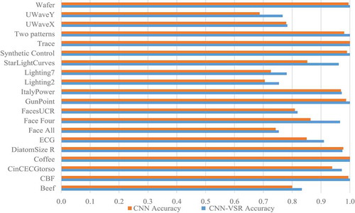
Based on the formulation of VSR, the training is stopped when the minimum error achieved for validation set, thus we expect to achieve the better accuracy for proposed CNN with VSR. To validate this, we plot the best-achieved accuracy on 20 UCR benchmark datasets with VSR and without VSR for the proposed architecture. It can be observed from Figure 7 that the accuracy produced by proposed architecture with VSR is marginally better than the proposed architecture without VSR for each selected dataset.

Figure 7. Comparison of accuracies with VSR and without VSR.

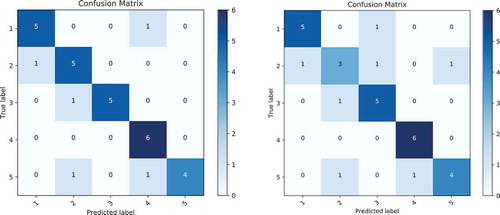
In Figure 8a,b, we present the confusion matrices yielded by the proposed CNN architecture with VSR and without VSR, respectively on Beef dataset. By comparing these confusion matrices in Figure 8a,b, it can be seen that there is bigger occurrence of confusion in Figure 8b. Further it is also evident from these figures that the class-wise classification accuracy for the proposed architecture with VSR is significantly better than the accuracy achieved without VSR. Furthermore, the similar observation can also be made for the other datasets.

Figure 8. Confusion matrices of proposed CNN model on Beef dataset.

Requirement of Early Stopping

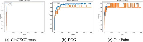
In this section, we discuss the requirement of other regularization method, named as: early stopping to avoid over-fitting. To demonstrate this, we have conducted empirical experiments and shown that the dropout regularization method is only helpful for few datasets such as CinCECGtorso (see Figure 9a). However from the Figure 9b,c, it is clear that this method is unable to tackle all the complexities in the data obtained through different applications such as ECG and GunPoint data, because these datasets are still prone to over-fitting. Moreover from the Figure 9b,c, it can be seen that the training accuracy is almost 100% and testing accuracy is lesser than training accuracy for ECG and GunPoint datasets. Therefore, we still require some other regularization method to tackle over-fitting in a variety of datasets; hence, the early stopping is required.

Figure 9. Training and testing accuracy curves.

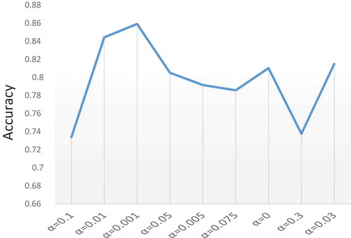
Effect of Modifying $\mathit{\alpha }$

The $\alpha$ defined in VSR is critical in deciding when to stop the learning process. Based on the definition of $\alpha$, large value may lead to too early stopping of learning process, which provides low generalization, and small value may increase the training time of learning process. Due to increase of high computing systems, higher generalization of the results is considered in finding out the optimal value of $\alpha$, which is required to reduce overfitting and underfitting in data. In order to analyze the effects of modifying $\alpha$ in learning process on the test accuracy of datasets, different values of $\alpha$ are used in VSR. The mean value (averaged over all datasets) of the testing set accuracy for different $\alpha$ has been plotted in Figure 10. As it is clearly inferred from the plot, for better generalization of trained results with unknown test set the lower values are achieving better generalization from training to testing process. Specifically, as shown in Figure 10, at $\alpha =0.001$ and $\alpha =0.01$, the best results are obtained for the tested datasets. Thus, these value of $\alpha$ should be taken into account. Moreover, it is worth to note that the selection of the most optimal value of $\alpha$ may depend upon other criteria as well. This optimal value of $\alpha$ heavily relies on the datasets and also on the problem addressed by the user for particular area in terms of accuracy and generalization.

Figure 10. Evolution of accuracy according to $\alpha$.

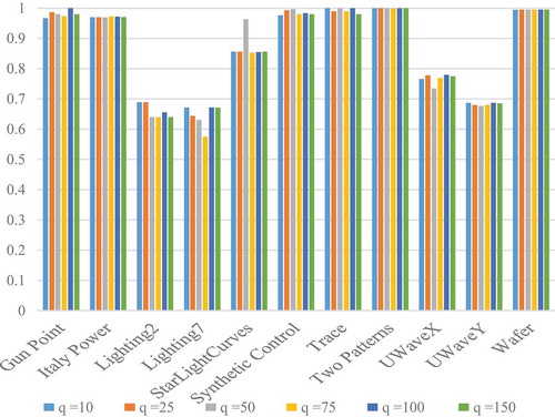
Effect of Modifying Patience $\mathit{q}$

The parameter $q$ denotes the number of epochs without improvement in validation loss, after which learning will not be continued. As such, with the aim of analyzing to what extent the results are affected by this parameter, we have carried out some experiments using different $q$ values based on proposed CNN-VSR architecture at $\alpha =0.001$.

Figure 11 reveals that there are no large difference between the obtained accuracies for different values of $q$. Furthermore, when the patience value is increased, the accuracies obtained on benchmark datasets become better. Moreover, the state of art comparison results clearly show that our proposed model is still competitive with the best available methods. It is also evident from Figure 11, at $q=50$ the accuracies of most datasets are better in comparison to other values of $q$, thus, $q=50$ can be recommended for conducting similar experiments on time series datasets with early stopping.

Figure 11. Accuracy values for the selected datasets, depending on the patience $q$.

Comparison with the State-of-art Methods

Final results after classification are presented in Table 3. As shown in Table 3, in 20 groups of datasets from UCR archive, CNN-VSR computed the best classification accuracies for most of the datasets. The rows of Table 3 are highlighted with three colors namely; Green, Red, and Yellow. These colors depict different meanings such as 1) Green color shows that the accuracy surpasses the best accuracy reported by UEA and UCR repository for particular dataset, 2) Yellow color shows that computed accuracy is competitive with best accuracy, and 3) Red color depicts that proposed architecture unable to achieve best accuracy. It can be easily observed from Table 3, that proposed architecture of CNN-VSR is the very competitive with other state of art algorithms. By using this architecture, we are able to achieve higher accuracy than best reported accuracy for 12 datasets. The main reason for achieving highest accuracy is that the CNN can extract and unwrap desirable internal structure, which is essential for generating deep structures. CNN can automatically generate these features by using a series of convolution and max-pooling operations.

Table 3. Comparison of accuracies of proposed CNN-VSR with the best available methods on UCR benchmark datasets.

Conclusion

In this article, a novel CNN-VSR architecture is proposed for univariate TSC. For this, a novel 2-D transformation approach is developed to convert 1-D time series of any length to 2-D matrix automatically. The implicit (early stopping) and explicit (dropout) regularization are applied, as time series signal is prone to over-fit as learning continues. Further, we have conducted a comparative empirical performance evaluation with the best available methods for individual benchmark datasets whose information are provided by UCR and UEA repository. We have performed the experiments on 20 benchmark datasets from UCR archive. Our results reveal that the proposed CNN-VSR architecture is competitive with the benchmark methods by achieving higher performance accuracy. Furthermore, it is demonstrated through experiments that stopping rule is able to enhance the performance of the proposed classifier. Moreover, we have also discussed the optimal model selection and analyzed the effects of different factors on performance of the proposed CNN-VSR architecture.

Acknowledgments

The authors are very grateful to Indian Institute of Information Technology Allahabad for providing the required resources. We would also like to thank the UCR archive for allowing access to the datasets used in this research.

Disclosure statement

No potential conflict of interest was reported by the authors.

References

- Acharya, U. R., S. L. Oh, Y. Hagiwara, J. H. Tan, M. Adam, A. Gertych, and R. S. Tan. 2017. A deep convolutional neural network model to classify heartbeats. Computers in Biology and Medicine 89:389–96. doi:10.1016/j.compbiomed.2017.08.022.
- Anders, U., and O. Korn. 1999. Model selection in neural networks. Neural Networks 12 (2):309–23. doi:10.1016/S0893-6080(98)00117-8.
- Antonucci, A., R. De Rosa, A. Giusti, and F. Cuzzolin. 2015. Robust classification of multivariate time series by imprecise hidden Markov models. International Journal of Approximate Reasoning 56:249–63. doi:10.1016/j.ijar.2014.07.005.
- Balkin, S. D., and J. Keith Ord. 2000. Automatic neural network modeling for univariate time series. International Journal of Forecasting 16 (4):509–15. doi:10.1016/S0169-2070(00)00072-8.
- Baydogan, M. G., G. Runger, and E. Tuv. 2013. A bag-of-features framework to classify time series. IEEE Transactions on Pattern Analysis and Machine Intelligence 35 (11):2796–802. doi:10.1109/TPAMI.2013.72.
- Bengio, Y. 2013. Deep learning of representations: Looking forward. In International Conference on Statistical Language and Speech Processing, Berlin, Heidelberg, 1–37. Springer.
- Bengio, Y., A. Courville, and P. Vincent. 2013. Representation learning: A review and new perspectives. IEEE Transactions on Pattern Analysis and Machine Intelligence 35 (8):1798–828. doi:10.1109/TPAMI.2013.50.
- Chen, H., P. Tino, A. Rodan, and X. Yao. 2014. Learning in the model space for cognitive fault diagnosis. IEEE Transactions on Neural Networks and Learning Systems 25 (1):124–36. doi:10.1109/TNNLS.2013.2256797.
- Chen, Y., E. Keogh, H. Bing, N. Begum, A. Bagnall, A. Mueen, and G. Batista. 2016. The UCR time series classification archive (2015). www.cs.ucr.edu/eamonn/time_series_data.
- Costa, Y. M. G., L. S. Oliveira, and C. N. Silla Jr. 2017. An evaluation of convolutional neural networks for music classification using spectrograms. Applied Soft Computing 52:28–38. doi:10.1016/j.asoc.2016.12.024.
- Cui, Z., W. Chen, and Y. Chen. 2016. Multi-scale convolutional neural networks for time series classification. arXiv preprint arXiv:1603.06995.
- Delgado, M., M. P. Cuellar, and M. C. Pegalajar. 2008. Multiobjective hybrid optimization and training of recurrent neural networks. IEEE Transactions on Systems, Man, and Cybernetics, Part B (Cybernetics) 38 (2):381–403. doi:10.1109/TSMCB.2007.912937.
- Esling, P., and C. Agon. 2013. Multiobjective time series matching for audio classification and retrieval. IEEE Transactions on Audio, Speech, and Language Processing 21 (10):2057–72. doi:10.1109/TASL.2013.2265086.
- Geman, S., E. Bienenstock, and R. Doursat. 1992. Neural networks and the bias/variance dilemma. Neural Computation 4 (1):1–58. doi:10.1162/neco.1992.4.1.1.
- Gurcan, M. N., H.-P. Chan, B. Sahiner, L. Hadjiiski, N. Petrick, and M. A. Helvie. 2002. Optimal neural network architecture selection: Improvement in computerized detection of microcalcifications. Academic Radiology 9 (4):420–29. doi:10.1016/S1076-6332(03)80187-3.
- Ijjina, E. P., and C. K. Mohan. 2016. Hybrid deep neural network model for human action recognition. Applied Soft Computing 46:936–52. doi:10.1016/j.asoc.2015.08.025.
- Jeong, Y.-S., M. K. Jeong, and O. A. Omitaomu. 2011. Weighted dynamic time warping for time series classification. Pattern Recognition 44 (9):2231–40. doi:10.1016/j.patcog.2010.09.022.
- Kate, R. J. 2016. Using dynamic time warping distances as features for improved time series classification. Data Mining and Knowledge Discovery 30 (2):283–312. doi:10.1007/s10618-015-0418-x.
- Keogh, E., and S. Kasetty. 2003. On the need for time series data mining benchmarks: A survey and empirical demonstration. Data Mining and Knowledge Discovery 7 (4):349–71. doi:10.1023/A:1024988512476.
- Kingma, D. P., and B. Jimmy 2014. Adam: A method for stochastic optimization. arXiv preprint arXiv:1412.6980.
- Längkvist, M., L. Karlsson, and A. Loutfi. 2014. A review of unsupervised feature learning and deep learning for time-series modeling. Pattern Recognition Letters 42:11–24. doi:10.1016/j.patrec.2014.01.008.
- LeCun, Y., Y. Bengio, and G. Hinton. 2015. Deep learning. nature. 521 (7553):436. Google Scholar doi:10.1038/nature14539.
- LeCun, Y., L. Bottou, Y. Bengio, and P. Haffner. 1998. Gradient-based learning applied to document recognition. Proceedings of the IEEE 86 (11):2278–324. doi:10.1109/5.726791.
- LeCun, Y. A., L. Bottou, G. B. Orr, and M. Klaus-Robert. 2012. Efficient backprop. In Neural networks: Tricks of the trade, 9–48. Berlin, Heidelberg: Springer.
- Lewis, D. D. 1998. Naive (Bayes) at forty: The independence assumption in information retrieval. In European conference on machine learning, Berlin, Heidelberg, 4–15. Springer.
- Li, H. 2015. On-line and dynamic time warping for time series data mining. International Journal of Machine Learning and Cybernetics 6 (1):145–53. doi:10.1007/s13042-014-0254-0.
- Lin, J., E. Keogh, L. Wei, and S. Lonardi. 2007. Experiencing SAX: A novel symbolic representation of time series. Data Mining and Knowledge Discovery 15 (2):107–44. doi:10.1007/s10618-007-0064-z.
- Lines, J., A. Bagnall, P. Caiger-Smith, and S. Anderson. 2011. Classification of household devices by electricity usage profiles. In International Conference on Intelligent Data Engineering and Automated Learning, Berlin, Heidelberg, 403–12. Springer.
- Prechelt, L. 2012. Early stoppingbut when?. In Neural networks: Tricks of the trade, 53–67. Berlin, Heidelberg: Springer.
- Rakthanmanon, T., B. Campana, A. Mueen, G. Batista, B. Westover, Q. Zhu, J. Zakaria, and E. Keogh. 2013. Addressing big data time series: Mining trillions of time series subsequences under dynamic time warping. ACM Transactions on Knowledge Discovery from Data (TKDD) 7 (3):10. doi:10.1145/2513092.
- Sak, H., A. Senior, and F. Beaufays. 2014. Long short-term memory based recurrent neural network architectures for large vocabulary speech recognition. arXiv preprint arXiv:1402.1128.
- Schäfer, P. 2015. The BOSS is concerned with time series classification in the presence of noise. Data Mining and Knowledge Discovery 29 (6):1505–30. doi:10.1007/s10618-014-0377-7.
- Schäfer, P. 2016. Scalable time series classification. Data Mining and Knowledge Discovery 30 (5):1273–98. doi:10.1007/s10618-015-0441-y.
- Schmidhuber, J. 2015. Deep learning in neural networks: An overview. Neural Networks 61:85–117. doi:10.1016/j.neunet.2014.09.003.
- Sezer, O. B., and A. M. Ozbayoglu. 2018. Algorithmic Financial Trading with Deep Convolutional Neural Networks: Time Series to Image Conversion Approach. Applied Soft Computing 70:525–38. doi:10.1016/j.asoc.2018.04.024.
- Uktveris, T., and V. Jusas. 2017. Application of convolutional neural networks to four-class motor imagery classification problem. Information Technology And Control 46 (2):260–73. doi:10.5755/j01.itc.46.2.17528.
- Wang, Z., W. Yan, and T. Oates. 2017. Time series classification from scratch with deep neural networks: A strong baseline. In Neural Networks (IJCNN), 2017 International Joint Conference on, 1578–85, Anchorage, Alaska, USA. IEEE.
- Weisstein, E. W. 1999. Convolution. Accessed November 30, 2018. http://mathworld.wolfram.com/Convolution.html.
- Wiens, J., E. Horvitz, and J. V. Guttag. 2012. Patient risk stratification for hospital-associated c. diff as a time-series classification task. In Advances in Neural Information Processing Systems, 467–75. Curran Associates Inc.
- Xing, Z., J. Pei, and E. Keogh. 2010. A brief survey on sequence classification. ACM Sigkdd Explorations Newsletter 12 (1):40–48. doi:10.1145/1882471.
- Zhao, B., L. Huanzhang, S. Chen, J. Liu, and W. Dongya. 2017. Convolutional neural networks for time series classification. Journal of Systems Engineering and Electronics 28 (1):162–69. doi:10.21629/JSEE.2017.01.18.
- Zheng, Y., Q. Liu, E. Chen, G. Yong, and J. Leon Zhao. 2016. Exploiting multi-channels deep convolutional neural networks for multivariate time series classification. Frontiers of Computer Science 10 (1):96–112. doi:10.1007/s11704-015-4478-2.