Handling Sequence-dependent Setup Time Flexible Job Shop Problem with Learning and Deterioration Considerations using Evolutionary Bi-level Optimization

ABSTRACT

Bi-level optimization is a challenging research area that has received significant attention from researchers to model enormous NP-hard optimization problems and real-life applications. In this paper, we propose a new evolutionary bi-level algorithm for Flexible Job Shop Problem with Sequence-Dependent Setup Time (SDST-FJSP) and learning/deterioration effects. There are two main motivations behind this work. On the one hand, learning and deterioration effects might occur simultaneously in real-life production systems. However, there are still ill posed in the scheduling area. On the other hand, bi-level optimization was presented as an interesting resolution scheme easily applied to more complex problems without additional modifications. Motivated by these issues, we attempt in this work to solve the FJSP variant using the bi-level programming framework. We suggest firstly a new bi-level mathematical formulation for the considered FJSP; then we propose a bi-level evolutionary algorithm to solve the problem. The experimental study on well-established benchmarks assesses and validates the advantage of using a bi-level scheme over the compared approaches in this research area to solve such NP-hard problem.

Introduction

Job shop scheduling problem (JSSP) is considered as the most active research field with the area of combinatorial optimization problems (Garey, Johnson, and Stockmeyer 1976). This problem holds a set of $n$ jobs that should be processed on $m$ specified machines. Each job consists of a specific set of operations, which must be processed according to a given order. Introduced by Nuijten and Aarts (1996), the FJSP is a generalization of the above-described definition, where each operation could be processed by a set of resources with a processing time that depends on the used resource. However, most classical FJSPs studied in the literature consider the known job processing times as a constant over time, which is not appropriate for many realistic situations, where the actual processing time of a job might increase or decrease regarding its normal processing time if it is scheduled later. This dynamic nature of job processing time may be the result of two situations: (1) The first one is where employees and machines execute the same job several times. They learn how to perform such operation more efficiently. In other words, the productivity is getting continuously better by performing similar tasks repeatedly. Accordingly, the processing time of a given job will be smaller if it is scheduled later in the sequence. In the literature, this phenomenon is known as learning effects (Wright 1936). Empirical studies in several industries have demonstrated that the learning effects have a significant impact on manufacturing systems. This phenomenon takes place mainly when the workers are able to perform setup, deal with both machine operations and software, such as read data or handle raw materials. The learning theory confirmed that the time needed to produce a single unit is in decreasing at a uniform rate. This latter is restrainedly related to the manufacturing process being observed. In this context, several works were suggested, for instance, the work of Wang and Cheng (2007), and Hosseini and Tavakkoli-Moghaddam (2013), etc. For more details, we refer the readers to the recent survey on scheduling problems with learning effects (Azzouz, Ennigrou, and Ben Said 2018). (2) The dynamic nature of the processing time is the result of a second situation in which it is called deterioration effects. It occurs when machines lose their performance during their execution times. In this case, the job that is processed later consumes more time than another one processed earlier. Scheduling in such environments is known as scheduling with deteriorating jobs, and it is first introduced by Gupta and Gupta (1988). The authors assumed that the processing time of all jobs is a function of their starting time. Since then, deterioration effects have widely studied in connection with scheduling problem.

Besides, bi-level programming problems are a special class of optimization problems with two levels of optimization tasks. These problems have been widely studied in the literature (Colson, Marcotte, and Savard 2007); and often appear in many practical problem solving tasks (Bard 2013). In practice, a bi-level scenario commonly occurs when a set of decision variables in an (upper level) optimization task is considered physically or functionally acceptable, only when it is a stable point or a point in equilibrium or a point satisfying certain conservation principles, etc. The satisfaction of one or more of these conditions is usually posed as another optimization task (lower level). Consequently, the bi-level scheme was presented as a new paradigm able to successfully solve a number of hierarchically NP-hard problems.

The particular structure of these optimization problems facilitates the formulation of several practical problems that involve a nested decision-making process. Motivated by this issue, we present in this paper, a new bi-level approach able to minimize the makespan criteria of the SDST-FJSP with learning/deterioration considerations. So far, we knew no other research was reported till date, where any variant of FJSP was addressed with bi-level optimization algorithm. Most of the researchers solved the problem as a single level optimization task. However, the nature of the problem fits quite well with the bi-level framework. To this end, we present in this work, a hierarchical structure of the problem such as a leader decision focuses on the assignment of jobs to machines, while a follower level is interested by the sequencement of operations. In other words, the leader assigns the jobs to machines and the follower sequences the jobs assigned to each machine. The main contributions of this paper are summarized as follows:

1. Proposing, a new bi-level evolutionary algorithm that we call (Bi-GTS) to solve SDST-FJSP with learning/deterioration effects.

2. Proposing a new mathematical bi-level formulation of the SDST-FJSP with learning/ deterioration effects, which will be evaluated using the bi-level proposed scheme.

3. Demonstrating the out-performance of our Bi-GTS over some of the most representative approaches with this research area which are VNS, TS, GA, and GTS on different commonly used benchmark problems from the literature.

FJSP Related Works

In recent years, FJSP has been highly studied by researchers. The problem could be decomposed into two sub-tasks: a routing sub-problem, which consists of assigning each operation to the available machine, and a scheduling sub-task, which consists in sequencing the assigned operations on all selected machines in order to optimize such considered objective function. Two kinds of approaches have been used to solve the problem: the hierarchical approach and the integrated one. Considering the first category, the routing sub-problem and the scheduling sub-problem are treated separately. The basic idea of this approach is to decomposing the original problem in order to reduce its complexity. Brandimarte (1993) used, for the first time, this approach for solving FJSP. He treated the routing sub-problem using several dispatching rules and then he solved the scheduling sub-problem using a tabu search algorithm. According to Brandimarte, the hierarchical scheme can be further expressed by information flow among the two sub-problems: in a one-way scheme, a routing problem is firstly solved, and then a sequencing problem is solved; alternatively, there is an iteration between the two steps, but the two tasks are evolved separately using then a correction stage. Following this architecture, Zribi, Kacem, and El Kamel (2004) solve the assignment problem using an heuristic algorithm and they apply a Genetic Algorithm (GA) to deal with the sequencing task. Another work in this field was reported by Saidi-Mehrabad and Fattahi (2007). Alternatively, the integrated architecture were used by considering assignment and scheduling at the same time. During the last few years, successful results have been achieved within integrated architecture such as the work of Ziaee (2014) and Azzouz, Ennigrou, and Ben Said (2017), etc.

The majority of researchers on scheduling assume that the setup time is negligible or is a part of the processing time. However, machine setup time is an important factor for production scheduling in several manufacturing systems; it may consume more than 20$\mathrm{\%}$ of available machine time (Pinedo 1995). In this way, there are two types of setup time: sequence-independent and sequence-dependent. In the first case, the setup time depends only on the job itself. However, in the second one, the setup time is not only dependent on the job but also on the previous job that ran on the same machine. Despite the relevance of the flexible job shop in real manufacturing systems, there is not many papers that consider both sequence-dependent setup-times and flexible job shop environments. We cite just the work of Saidi-Mehrabad and Fattahi (2007) which presented a TS for solving the SDST-FJSP to minimize the makespan. Moreover, Bagheri and Zandieh (2011) proposed a variable neighborhood search based on integrated approach to minimize an aggregate objective function (AOF) where $AOF=\alpha F1+(1-\alpha )F2$ and $\alpha$ denote the weight given, respectively, to makespan $(F1)$ and mean tardiness $(F2)$. The most recent comprehensive survey of scheduling problem with setup times is given by Allahverdi (2015).

Bi-level Optimization: Basic Definition

As we mentioned previously, bi-level optimization is an important research area of mathematical programming (Dempe 2002). This type of problem has emerged as an important area for progress in handling many real-life problems in different domains, e.g.,, optimal control, process optimization, game-playing strategy development, transportation problems (Chaabani, Bechikh, and Said 2015b). The first formulation of bi-level programming was proposed in 1973 by Bracken and McGill (1973). After that, Candler and Norton (1977) are the first authors who use the designation of bi-level and multi-level programming with optimization problem. The decision variables of a bi-level optimization problem (BOP) are split into two groups that are controlled by two decision makers called leader (on the upper level) and follower (on the lower level). Both decision makers have an objective function of their own and a set of constraints on their variables. Furthermore, there are coupling constraints that connect the decision variables of leader and follower. The nested structure of the overall problem requires that a solution to the upper level problem may be feasible only if it is an optimal or near-optimal solution to the lower level problem.

Using this description, we present in the following the bi-level SDST-FJSP with learning and deterioration consideration formulation. Then, we describe the bi-level evolutionary algorithm to solve the problem.

A New Bi-level Mathematical Model for SDST-FJSP with Learning and Deterioration Considerations

The SDST-FJSP with learning and deterioration effects consists on performing $n$ jobs on $m$ machines. The set of machines is noted $M$ $(M=M_1,..M_k)$. Each job $i$ consists on a sequence of $n_i$ operations (routing). Each routing has to be performed to complete a job. The execution of each operation $j$ of a job $i$ noted ($O_{ij}$), requires one machine out of a set of a given machines $M_{i,j}$ (i.e., $M_{i,j}$ is the set of machines available to execute $O_{ij}$). The problem is to define a sequence of operations together with the assignment of start times and machines for each operation. It is noteworthy that the following assumptions are considered in this paper:

• Jobs are independent of each other;

• Machines are independent of each other;

• One machine can process at most one operation at a time;

• No preemption is allowed;

• All jobs are available at time zero;

• The applied time deterioration rate is as follows:

(1) $P_{ijk}^{\prime }=P_{ijk}(1+\beta t)$(1)

where $P_{ijk}^{\prime }$ is the actual processing time for $O_{ij}$ on $k^{th}$ machine and $P_{ijk}$ is a normal processing time, $t$ is the starting time of the operation and $\beta$ is a non-negative deterioration index.

• Setup times are dependent on the sequence of jobs. When one of the operations of a job $t$ is processed before one of those of job $i$$(t$$\ne i)$ on machine $M_k$, the sequence depend setup time is $S_{t,i,k}$$>$$0$.

• The applied position based learning effect is defined as follows:

(2) $S_{t,i,k,r}^{\prime }=S_{t,i,k}{r}^a$(2)

where $S_{i,k,r}^{\prime }$ corresponds to the actual SDST for $i^{th}$ jobs on $K^{th}$ machine and $S_{i,k}$ is the normal SDST. We should mention here that the standard FJSP can be classified into two main categories: (1) the Total-FJSP (T-FJSP), and (2) the Partial-FJSP (P-FJSP) (Kacem, Hammadi, and Borne 2002). In T-FJSP, each operation can be processed by all machines. However, in P-FJSP, at least one operation may not be processed on all machines. Several researches pointed out that the P-FJSP is more general and complex as compared to T-FJSP on the same scale. In this paper, we consider the P-FJSP.

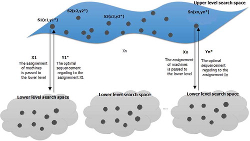
According to this description, we present in the following a hierarchical structure of the SDST-FJSP problem with learning/deterioration effects taking into account the presented assumptions and constraints. In fact, a leader decision level focuses on the assignment of jobs to machines, while a follower is interested by the sequencement of operations. In this regard, the leader’s objective depends only on its’ variables. (cf. Figure 1). However, the feasibility of a solution depends on the follower’s response as well. It is important to note that the main motivation behind the design of SDST-FJSP as a bi-level model is the possibility to well accelerate the diversity and the convergence of the search by exploring more job assignments in the upper level search space and then concentrates on one fixed assignment at each way, in order to found the corresponding optimal job sequencement. We seek then to enhance the search ability on the SDST-FJSP decision space in order to improve the quality of solutions. We give in the following, the used parameters and the decision variables used in our formulation:

$n$ the number of jobs,

$m$ the number of machines,

$i,i^{\prime }$ index for jobs where $i\in \{1,2,..n\}$,$i^{\prime }\in \{0,\mathrm{1...},n\}$,

$j,j^{\prime }$ index for operations of job$$$i$,

$k$ index of machines where $k\in \{1,2,..n\}$,

$J$ the set of jobs,

$M$ the set of machines,

$O_i$ the set of operations of a job $i$,

$O_{ij}$ the $j^{th}$ operation of job $i$,

$e_{ijk}$ takes value 1 if machine i is eligible for $O_{ij}$ and 0 otherwise,

$M_{ij}$ the set of alternative machines in which operation $ij$ can be processed, ($M_{ij}$$\subseteq$$M$),

$M_{ij}\cap M_{i^{\prime }{j}^{\prime }}$ the set of machines by which operations $O_{ij}$ and $O_{i^{\prime }{j}^{\prime }}$ can be processed,

$S_{ijk}$ the normal sequence-dependent setup time (SDST) of operation $O_{ij}$ on machine $k$,

$S_{ijk}^{\prime }$ the actual SDST of operation $O_{ij}$$$on machine $k$,

$C_i$ the completion time of a job $i$,

$C_{ijk}$ the completion time of an operation $O_{ij}$ on machine $k$,

$C_{max}$ maximum completion time over all jobs (makespan),

$r$ the position of operation in the sequence,

$\alpha$ learning index where $\alpha <0$,

$p_{ijk}$ the normal processing time of operation $O_{ij}$ on machine $k$,

$p_{ijk}^{\prime }$ the actual processing time of operation $O_{ij}$$$on machine $k$,

$\beta$ the deterioration rate

$L,$ a large number.

The proposed mathematical model is defined as follows:

Decision variables

$X_{ijk}=\left\{\begin{array}{c}1if>machine>k>is>selected>for>operation>O_{ij},\\ 0otherwise\end{array}\right.$

$Y_{ij{i}^{\prime }{j}^{\prime }k}=\left\{\begin{array}{c}1if>operation>O_{ij}>precedes>operation>O{i}^{\prime }{j}^{\prime }>\\ on>machine>k,\\ 0otherwise\end{array}\right.$

The upper level constraints are defined as follows: constraint (1) describes that each operation $O_{ij}$ should be assigned to only one machine. Secondly, they specify that each operation is assigned to one of its eligible machines (on constraint (2)). Regarding to the lower level part, we consider eight constraints related to the sequencement of jobs on the different machines. Constraint (3) ensures that every operation could have at most one succeeding operation. Constraint (4) ensures that the dummy operation is the first one on machines. Constraint (5) assures that each operation has exactly one preceding operation on the same machine. Constraints (6) and (7) define the learning and deterioration formulas taken into consideration in this model. Constraint (8) guarantees that one machine cannot process two different operations simultaneously. In other words, the difference between the completion times of two consecutive operations on one machine should be greater than the setup time plus the processing time of the operation processed later. In fact, the constraint (9) ensures that the precedence relationships between operation $O_{ij}$ and $O_{i{j}^{\prime }}$ of a job should be satisfied. Thus, operation $O_{ij}$ cannot start before the operation $O_{ij-1}$ terminates its processing. The constraint (10) defines the completion times of the jobs, and finally, constraint (11) establishes the makespan parameter.

Figure 1. SDST-FJSP problem with learning effect formulated as bi-level optimization problem.

Bi-GTS Basic Scheme

As we have mentioned previously, the two main goals of this work are: (1) modeling SDST-FJSP with learning/deterioration effects problem using the bi-level optimization programming and, (2) designing a bi-level evolutionary strategy able to improve the resolution efficiently of this problem. In this work, we handle two types of meta-heuristics: a local optimization method based on Tabu Search (TS) with a global optimization approach based on GA, at both levels. The GA was applied in the upper level in order to better explore the whole search space and then to direct the algorithm into the region representing the best assignment vector. Our choice of the GA relies on the fact that this latter represents an evolutionary based algorithm, simple and powerful, able to solve complex combinatorial problem such as scheduling problem. In fact, the lower level problem was handling using the TS method, accentuating then the convergence rate of the procedure in the lower level space. The TS determines the optimal scheduling of the $n$ jobs on the $M$ machines according to the upper decision variables (i.e., optimized assignment). To this end, the bi-level decision-making process is performed as follows. First, the GA process makes his decision and fixes the values of his upper variables (i.e., by applying selection, recombination, and mutation operators which are presented in the following subsections). After that, the follower reacts by setting his variables according to the ones fixed by the GA in the upper level. The leader has perfect knowledge of the follower’s scenario (objective function and constraints) and also of the follower’s behavior. The follower observes the leader’s action (the generated assignment), and then optimizes his own objective function subject to the decisions made by the leader (and subject to the imposed constraints). As the leader’s objective function depends on the follower’s decision, the leader must take the follower’s reaction into account (cf. Figure 2). To more understand the bi-level process, we present in the following the step-by-step procedure of our proposed algorithm.

Figure 2. Bi-GLS basic scheme.

Upper Level Optimization Procedure

Step 1 (Initialization Scheme): We generate an initial parent population of $N$ assignments randomly. Then, the lower level optimization procedure is executed to identify the optimal sequencements according to such generated affectation. In fact, the upper level fitness is assigned based on both upper level function value and constraints since the lower level problem appears as a constraint to the upper level one. In this paper, the upper solution is coded using a binary matrix proposed by Azzouz, Ennigrou, and Jlifi (2015) where the rows represent the job operations and the columns correspond to the used machines as described in Figure 3.

Step 2 (Upper level parent selection): We choose $(N/2)$ members from the parent population using tournament selection operator.

Step 3 (Variation at the upper level): We perform crossover and mutation operators in order to create the upper offspring population. In this way, we use the crossover operator order 1 (Davis 1985) which consists on selecting randomly two positions $X{P}_1$ and $X{P}_2$ in the parent 1. Subsequently, the middle part is copied to the first offspring. The rest of this child is filled from the parent 2 starting with position $X{P}_2+1$, and jumping elements that are already presented in the offspring 1. The same steps are repeated for the second offspring by starting with the parents 2. Figure 4 shows an example of this technique. Till now to the mutation operator, we use the mutation technique proposed by Pezzella, Morganti, and Ciaschetti (2008) in which, we select one operation with the maximum workload (i.e. the maximum amount of work that a machine produces in a specified time period). Then we assign to the machine the minimum workload it if possible.

Step 4 (Lower level optimization): We solve the lower level optimization problem for each generated offspring using the tabu search algorithm (cf. the following subsection).

Step 5 (Offspring evaluation): We combine both upper level parents (the assignments in our case) and the upper level children into an $R_t$ population and we evaluate them based on the upper level objective function and the constraints.

Step 6 (Environmental selection): We fill the new upper level population using a replacement strategy. The new upper level population is formed with the $N$ best solutions of $R_t$ set. If the stopping criterion is met then return the best upper level solution; otherwise, return to Step 2.

Lower Level Optimization Procedure

The tabu search strategy is considered as an intensification procedure able to guide the search in order to explore the solution space beyond local optimality. It has achieved widespread success in solving practical optimization problem. In this paper, we opt to use such algorithm in order to optimize the sequencement of operation jobs according to the passed assignment upper solution. The step-by-step procedure of the lower level TS algorithm is described as follows:

Step 1 (Initial solution): We need to generate firstly an initial solution. This latter is created based on the passed upper level solution structure. In this way, we conserve the same upper solution representation, while considering now the operation order in the matrix as the scheduling of operation on the $M$ machines.

Step 2 (Generate neighborhood): In this step, we determine the neighborhood of the current solution. Then, we define two types of moves: (1) the swap of two critical operations, and (2) the reassignment of an operation. Denote that a critical path is the longest path in the schedule composed of operations related either by precedence or disjunctive constraints. We determine then, the neighborhood of the current solution and we evaluate it to be able to choose the best non-tabu neighbor satisfying the aspiration criterion. It is important to note here that the best solution will be stored in an elite list. Then, any solution belongs to the neighborhood of the current one that obeys the following condition (if the difference costs between the current and the best one is less than or equal to $\epsilon$ such as $\epsilon >0$), will be stored in a secondary elite list.

Figure 3. A sample chromosome encoding by our representation.

Figure 4. Order 1 crossover operator with $X{P}_1=3$ and $X{P}_2=7$.

Step 3 (Neighborhood evaluation): In a tabu search method, the best non-tabu neighbor belonging to the current solution neighborhood will be selected for the next iteration. Hence, all neighbors must be evaluated in order to determine the best one. However, a global evaluation, i.e. computation of all start times of all operations, of each neighbor will need a considerable time. For this reason, we propose an estimation method in which only a subset of operations will be taken into account and to which start times will be recalculated. These operations are the ones effectively concerned by the move executed. Once the current neighbor was chosen, the move will be stored in the tabu list. Thereafter, the corresponding selected move is applied to the offspring solution that will be stored as elite solution. Subsequently, the lower level fitness is assigned based on the lower level objective function and constraints.

Step 4 (Diversification technique): In order to avoid that a large region of the search space remains completely unexplored, it is important to diversify the search during the optimization process. For this reason, we use three diversification techniques as follows:

• Select randomly a solution among the elite solution list,

• Select randomly a solution from the secondary elite solution list, or

• Create a new solution by re-sequencing the operations of one job selected randomly.

Each of them is executed when the number of iterations performed after the last diversification phase or the last improving iteration exceeds a predefined threshold (the diversification probability).

Step 6 (Stop criterion): If the stopping criterion is met then we send the best found lower level solution to the upper level problem; otherwise, return to Step 2.

Experimental Study

The main motivation of this paper is to investigate the performance of the bi-level scheme with both problems (1) the SDST-FJSP with the learning effects and (2) the SDST-FJSP with learning/deterioration effects. Thus, two parts are considered in this experimental study. In the first one, we will try to evaluate the performance and the superiority of our Bi-GTS regarding four different schemes within this research area that are:

1. Variable Neighborhood Search (VNS) which explores distant neighborhoods based on a variable neighborhood changes proposed by Bagheri and Zandieh (2011);

2. Tabu search (TS) algorithm which is a based-intensification technique proposed by Ennigrou and Ghedira (2008);

3. Genetic algorithm which is an evolutionary method proposed by Azzouz, Ennigrou, and Said (2016);

4. Hybrid genetic algorithm coupled with VNS algorithm (GTS) (Azzouz, Ennigrou, and Ben Said 2017).

The second part of this experimental study focus on evaluating our Bi-GTS on the SDST-FJSP with learning and deterioration effects. We should mention here that only the work of Tayebi Araghi and Rabiee (2014) was reported to solve this problem. For this reason, we will use the same experimental framework presented in this latter to access the performance of our proposal. To this end, the second part focus mainly on a comparative study of the Bi-GTS algorithm to the following methods:

1. GA version adapted to the SDST-FJSP with learning and deterioration effects proposed by Pezzella, Morganti, and Ciaschetti (2008),

2. VNS which version adapted to the SDST-FJSP with learning and deterioration effects proposed by Amiri et al. (2010), and

3. GVNSWAF which is an hybrid algorithm based on GA coupled with VNS search strategy with affinity function proposed by Tayebi Araghi and Rabiee (2014).

We note that all simulations are performed on the same machine (Intel Core i5-3230 CPU 2.6 GHz and 6 GB RAM). The remaining of this section is organized as follows: Subsection 5.1 presents the used benchmarks and metrics used in this study. The second subsection devoted the parameter tuning and settings. Then, we report the comparative results with (1) SDST-FJSP with learning effects, and (2) SDST-FJSP with learning and deterioration effects.

Used Benchmarks and Metrics

In this subsection, we describe the different benchmark problems used in our experimental study. In fact, we choose commonly used test problems within the community that allow assessing the performance of any used algorithm with respect to different kinds of difficulties. Thus, two kinds of benchmarks are adopted: The first one is adopted to evaluate the SDST-FJSP with learning effects which is denoted $SDST-HUdata$ (González, Rodriguez Vela, and Varela 2013). It contains $20$ instances derived from the first $20$ instances of the FJSP benchmarks proposed by Hurink, Jurisch, and Thole (1994). Each instance was created by adding to the original instance one setup time matrix $S_{t,k}$ for each machine $k$. The same setup time matrix was considered for all benchmark instances. Each matrix has a size of $n\times n$, and the $S_{t,i,k}$ value indicates the setup time needed to reconfigure the machine $k$ when it switched from job $t$ to job $i$. These setup times are sequence dependent and they fulfill the inequality triangle. The second set of benchmarks consists on $18$ instances proposed by Tayebi Araghi and Rabiee (2014). For each job, three combinations of maximum operation ($OpMax$) and machines are considered. Table 1 summarizes the characteristics of the used benchmarks. To evaluate now the generated results and to compare the performance of the used algorithms, we use two kinds of metrics: (1) the first one is the makespan parameter which denotes the completion time of the last operation and (2) the second performance measure is the relative percentage deviation (RPD) which is calculated as follows:

(3) $RPD=\frac{so{l}_{algo}-so{l}_{min}}{so{l}_{min}}\times 100$(3)

Table 1. Description of Tayebi Araghi et al., instances (Tayebi Araghi and Rabiee 2014).

Factors	Values
Number of Jobs ($N$)	small: $5$, $10$, $15$, $20$, $25$
	large: $40$
Combination of number of maximum operation per job and number of machines	small: $5\times 2,10\times 315\times 4$
	large: $20\times 6,30\times 840\times 10$
Processing time ($P_{ijk}$)	U($1$, $50$)
Setup times($S_{ijk}$)	U($1$, $25$)

where $So{l}_{algo}$ is the makespan of each algorithm and $so{l}_{min}$ is the best solutions obtained for each instance after ten iterations.

Parameter Tuning and Settings

It is well known that the performance of an algorithm is heavily dependent on the setting of control parameters. Most research use fixed parameter values after some preliminary experiment or with reference to values of the previous similar literature. In this context, the most popular-used approach is the full factorial experiment (Ruiz, Maroto, and Alcaraz 2006). This later is usually used when the number of factors and their levels are small. Consequently, the major inconvenient of this method exists when the number of factors and their level are large. In such situation, it’s well difficult to calculate all possible combinations. Thus, the Taguchi's design of experiment (TDOE) approach was represented as an interesting alternative able to reduce the number of required tests. TDOE suggests the use of orthogonal arrays to organize the parameters affecting the process and the levels at which they should be varying. Orthogonal arrays can be used to accomplish optimal experimental designs by considering a number of experimental situations (Roy 2001). Moreover, the Taguchi method uses the signal-to-noise ratio (SNR), instead of the average value to interpret the data (experimental results). SNR can reflect both the average and the variation of the quality characteristic. In this way, the Taguchi’s method classifies the objective functions into three groups: (1) the smaller-the-better type, (2) the larger-the-better type and (3) the nominal-is-the best type. Since almost all objective functions in scheduling are categorized in the smaller the-better type, its corresponding SNR is expressed as follows:

(4) $SNR=-{log}_{10}(\frac{1}{n}\sum _{i=10}^n(objectivefunction{)}_i^2)$(4)

Before the calibration of the Bi-GTS, the algorithm is subjected to some preliminary tests to obtain the proper parameter levels to be tested in the fine-tuning process. In order to achieve more accurate and stable results for our proposed algorithm, we considered five parameters for tuning. These parameters are $P_{cross}$, $P_{mut}$, $po{p}_{size}$, $MaxI{t}_{GA}$ and $MaxI{t}_{TS}$. These parameters with their levels are shown in Table 2. The corresponding orthogonal array with five factors and three levels in Taguchi method is $L_{27}$. By analyzing all of experimental results using Taguchi method, the average SNR and average maximum completion time were obtained for the considered experiments. Figure 5 displays the obtained results. In this way, the optimal levels are A(2), B(3), C(3), D(3) and E(2) (cf.Figure 5). Furthermore, results computed in terms of mean makespan in Taguchi experimental analysis confirmed the optimal levels obtained using SNR values (see Figure 6). Table 3 exhibits the effectiveness rank of parameters in minimizing makespan.

Figure 5. The SNR plot for experiments in Taguchi methodology.

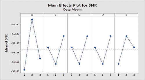
Figure 6. The plot of means of makespan for experiments in Taguchi methodology.

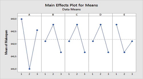
Table 2. Parameters and their levels.

	A$P_{cross}$	B$P_{mut}$	C$po{p}_{size}$	D$MaxI{t}_{GA}$	E$MaxI{t}_{TS}$
High(1)	0.8	0.8	150	120	200
Medium (2)	0.5	0.5	80	80	150
Low(3)	0.2	0.2	60	50	100

Table 3. SNR table for experiments.

level	A	B	C	D	E
1	−56,16	−56,15	−56,15	−56,15	−56,16
2	−56,14	−56,16	−56,16	−56,16	−56,15
3	−56,16	−56,15	−56,15	−56,15	−56,15
Delta	0,03	0,01	0,01	0,01	0,01
Rank	1	3,5	3,5	3,5	3,5

Table 4. Makespan values of Bi-GTS, VNS, TS, GA and GTS on SDST-HUdata benchmarks. The symbol ” + ” means that $H_0$ is rejected while the symbol ” – ” means the opposite. The best values are highlighted in bold.

Instance Problem	Size$(n\times m)$	flexibility	Bi-GTS	GTS	GA	TS	VNS
La1	$10\times 5$	$1.15$	641 (++++)	641 (++++)	721 (++++)	814 (+++ -)	721 (+++ -)
La2			734 (++++)	780 (++++)	871 (+++ -)	854 (++++)	908 (++-+)
La3			606 (++++)	643 (++++)	768 (++++)	686 (++++)	818 (++++)
La4			620 (++++)	694 (++++)	794 (+++ -)	732 (++++)	774 (++ – +)
La5			540 (++++)	560 (++++)	613 (++ – +)	623 (++ – +)	726 (++++)
La6	$15\times 5$	$1.15$	885 (- +++)	927 (- + – +)	1055 (++++)	934 (++ – +)	1069 (++++)
La7			815 (++++)	855 (++++)	1034 (++++)	891 (++++)	1080 (++++)
La8			870 (++++)	969 (++ – +)	1132 (++++)	988 (+ – ++)	1102 (++++)
La9			932 (- +++)	932 (- +++)	1053 (++++)	1015 (++++)	1106 (++++)
La10			891 (- +++)	907 (- +++)	1052 (++++)	947 (++++)	1077 (++++)
La11	$20\times 5$	$1.15$	1157 (++++)	1159 (++++)	1388 (++++)	1241 (++++)	1446 (++++)
La12			1006 (++++)	1024 (++++)	1267 (++++)	1089 (++++)	1409 (++++)
La13			1083 (++++)	1092 (++++)	1300 (++++)	1118 (++++)	1354 (++++)
La14			1167 (- +++)	1183 (- +++)	1340 (++++)	1245 (++++)	1402 (++++)
La15			1283 (- +++)	1286 (- +++)	1626 (+++ -)	1401 (++++)	1629 (++ – +)
La16	$10\times 10$	$1.15$	1018 (++++)	1051 (++++)	1282 (++++)	1099 (++++)	1310 (++++)
La17			802 (++++)	843 (++ – +)	999 (++++)	846 (+ – ++)	1046 (++++)
La18			913 (++++)	949 (++++)	1192 (++++)	1000 (++++)	1160 (++++)
La19			928 (++++)	1004 (++++)	1174 (++++)	1089 (++++)	1224 (++++)
La20			926 (++++)	1006 (++++)	1190 (++++)	1074 (++++)	1224 (++++)

Adopted Statistical Methodology

In order to compare between the algorithms, we choose to use the Wilcoxon rank sum test in a pairwise fashion (Derrac, García, Molina, and Herrera 2011). It allows to verify whether the results are statistically different or not between samples. Thus, we perform $30$ runs for each couple (algorithm, problem) with different random seeds (i.e., $30$ different randomly generated populations). Once the results are obtained, we use the MATLAB ranksum function in order to compute the p-value of the following hypothesis: (1) $H_0$: median (Algorithm1) = median (Algorithm2) and (2) $H_1$: median (Algorithm 1) $\ne$ median (Algorithm 2) for a confidence level of 95%, if the p-value is found to be less or equal than $0.05$, we reject $H_0$ and we accept $H_1$. In this way, we can say that the medians of the two algorithms are different from each other and that one algorithm outperforms the other viewpoint the used metric. However, if the p-value is found to be greater than $0.05$, then we accept $H_0$ and we cannot say that one algorithm is better than the other nor the opposite.

Comparative Results of the SDST-FJSP with Learning Effects

In order to validate the advantage of the bi-level scheme in solving the SDST-FJSP with learning effects, we compared our model regarding four mono-level different schemes. The simulation results are summarized in Table 5. The instance names are listed in the first column, the second column shows the size $(n\times m)$ of each instance. The remaining columns report the obtained results of the used algorithms. We observe from Table 5 that Bi-GTS presents the best performance on the majority of test problems. It outperforms GTS, GA, TS, and VNS on $19$ benchmark problems. This fact can be explained by the driving force of Bi-GTS in manipulating both diversity and convergence under the search space. In this way, the bi-level scheme was able at first to explore more possible assignments in the upper level search space. Then, the algorithm accentuates the search in the lower level regarding all possible generated assignments in the other level to be able to generate good bi-level solution qualities.

Table 5. RPD values of Bi-GTS, VNS, TS, GA and GTS on SDST-HUdata benchmarks.

Instance Problem	BI-GTS	GTS	GA	TS	VNS
La01	0	0.02	1.55	7.36	2.11
La02	0.15	0.61	0.96	8.53	1.98
La03	0.39	1.06	1.64	5.33	2.31
La04	0.41	4.43	0.85	3.66	3.25
La05	0.75	0.11	1.89	3.58	2.11
La06	0.55	2	0.51	2.79	3.46
La07	0.40	1.63	0.62	2.99	2.01
La08	0	0.46	0.57	2.41	1.91
La09	0	2.26	1.41	3.21	3.48
La10	0	5.15	1.68	4.02	0.93
La11	0.26	2.92	1.01	2.08	1.80
La12	0.11	2.73	0.82	2.71	3.12
La13	0	2.18	0.93	3.14	3.08
La14	1.37	1.93	2.10	1.76	3.81
La15	1.08	7.23	1.41	1.18	1.88
La16	0.14	0.73	0.54	4.04	1.83
La17	1.02	1.94	3.31	2.39	1.89
La18	0.2	1.56	0.99	5.81	2.95
La19	0.1	1.4	2.94	6.67	1.47
La20	0.2	3.5	0.75	9.36	1.88
Average	0.35	2.19	1.32	4.15	2.36

In addition to the empirical simulation presented to access the performance of the different approaches, we use Relative Percentage Deviation (RPD) as a common performance metric to measure the algorithm stability. Table 6 reports the generated results of the algorithms. In fact, we deduce that the proposed Bi-GTS outperforms the other algorithms in $18$ instances with an average RPD value of $0.35$. 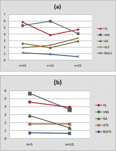The worst performance is then observed with the TS algorithm which presents an average RPD value of $\mathrm{4.15.}$ To further evaluate the performance of our algorithm, we study the interaction between the performance of the algorithm regarding the problem dimension. Figure 7 presents a plot describing the average RPD trace of the used approaches regarding to the number of jobs and machines, respectively. According to this Figure, we remark that Bi-GTS seems competitive regarding to other approaches. In fact, it generates the better RPD values on small, average, and large-scale problems. As well, we observe from these figures that the other approaches are sensitive to the number of machines. They represent a bad RPD values regarding to a variation on the machine numbers. Thus, we can deduce that the Bi-GTS keeps its robust performance in different problem sizes and especially with large-scale problem instances.

Table 6. Makespan values of Bi-GTS, GTS, GAVNS, GA and VNS on Tayebi benchmarks. The best values are highlighted in bold.

Instance problem	Bi-GTS	GTS	GVNSWAF	GA	VNS
5-5-2	213	236	262	281	331
5-10-3	247	264	279	339	350
5-15-4	316	377	323	524	696
10-5-2	371	409	472	491	576
10-10-3	570	649	681	843	1031
10-15-4	633	691	365	781	689
15-5-2	727	740	749	812	916
15-10-3	784	851	859	1203	1273
15-15-4	941	1110	661	1140	1151
20-5-2	1243	1294	1281	1439	1604
20-10-3	1453	1572	1464	2014	2157
20-15-4	1502	1790	1611	2063	2329
25-5-2	1185	1310	1288	1547	1533
25-10-3	2022	2306	1922	2515	2500
25-15-4	2253	2501	1813	2694	2576
40-20-6	3675	3712	3802	4304	4736
40-30-8	4172	4246	4781	5466	5765
40-40-10	5330	5535	6408	7688	8126

Comparative Results of SDST-FJSP with Learning and Deterioration Effects

In this second part, we are interesting to compare our bi-level algorithm mainly to the GVNSWAF work since it is the only one that is proposed to handle the same problem interest. Table 4 shows the obtained results in terms of makespan values. In particular, we indicate that the instance problem names follow the $(n-OpMax-m)$ formula in which $n$ represents job number, $OpMax$ is the maximum operation number considered for each jobs and the $m$ value defines the number of machines detained by the problem. We observe from this Table that our Bi-GTS outperforms also the other algorithms on fourteen/eighteen instances. The second best value is observed by the GVNSWAF and GTS which they outperform the other algorithms (GA and VNS) in nine instances. Thus, we can properly say that the hierarchical scheme allows to generate good solutions which confirms that this scheme is more adapted to solve the SDST-FJSP with learning and deterioration considerations than the other compared approaches.

Figure 7. The average RPD vaues of the used algorithms regarding to (a) the number of jobs and (b) the number of machines respectively.

Conclusion and Future Works

In this paper, we consider two realistic assumptions with the flexible job shop problem (FJSP), namely, the sequence-dependent setup times (SDST) and the learning/deterioration effects. We have suggested, for the first time, a bi-level evolutionary algorithm to solve this problem. The experimental results revealed that Bi-GLS is very competitive with respect to the considered algorithms. As part of our future work, we plan firstly to improve the proposed bi-level scheme by testing other meta-heuristic approaches. Secondly, the obtained results are promising, thus it would be a challenging perspective to investigate the dynamic SDST-FJSP with learning/deterioration effects, in order to reflect as closely as possible the reality of the actual flexible manufacturing systems.

References

- Allahverdi, A. 2015. The third comprehensive survey on scheduling problems with setup times/costs. European Journal of Operational Research 246:345–78. doi:10.1016/j.ejor.2015.04.004.
- Amiri, M., M. Zandieh, M. Yazdani, and A. Bagheri. 2010. A variable neighbourhood search algorithm for the flexible job-shop scheduling problem. International Journal of Production Research 48 (19):5671–89. doi:10.1080/00207540903055743.
- Azzouz, A., M. Ennigrou, and L. Ben Said. 2017. A hybrid algorithm for flexible job-shop scheduling problem with setup times. International Journal of Production Management and Engineering 5 (1):23–30. doi:10.4995/ijpme.2017.6618.
- Azzouz, A., M. Ennigrou, and L. Ben Said. 2018. Scheduling problems under learning effects: Classification and cartography. International Journal of Production Research 56 (4):1642–61. doi:10.1080/00207543.2017.1355576.
- Azzouz, A., M. Ennigrou, and B. Jlifi. 2015. Diversifying ts using ga in multi-agent system for solving flexible job shop problem. Proceedings of the 12th International Conference on Informatics in Control, Automation and Robotics (ICINCO), France, vol. 1, 94–101.
- Azzouz, A., M. Ennigrou, and L. B. Said. 2016. Flexible job-shop scheduling problem with sequence-dependent setup times using genetic algorithm. 18th International Conference on Enterprise Information Systems (ICEIS), Italy, vol. 2, 47–53.
- Bagheri, A., and M. Zandieh. 2011. Bi-criteria flexible job-shop scheduling with sequence-dependent setup times—variable neighborhood search approach. Journal of Manufacturing Systems 30 (1):8–15. doi:10.1016/j.jmsy.2011.02.004.
- Bard, J. F. 2013. Practical bilevel optimization: Algorithms and applications, vol. 30. Springer Science & Business Media.
- Bracken, J., and J. T. McGill. 1973. Mathematical programs with optimization problems in the constraints. Operations Research 21 (1):37–44. doi:10.1287/opre.21.1.37.
- Brandimarte, P. 1993. Routing and scheduling in a flexible job shop by tabu search. Annals of Operations Research 41 (3):157–83. doi:10.1007/BF02023073.
- Candler, W., and R. Norton. 1977. Multilevel programming. Technical Report 20, World Bank Development Research, Washington, D. C.
- Chaabani, A., S. Bechikh, and L. B. Said. 2015b. A co-evolutionary decomposition-based algorithm for bi-level combinatorial optimization. 2015 IEEE Congress on Evolutionary Computation (CEC), IEEE, Japan, 1659–66.
- Colson, B., P. Marcotte, and G. Savard. 2007. An overview of bilevel optimization. Annals of Operations Research 153 (1):235–56. doi:10.1007/s10479-007-0176-2.
- Davis, L. D. 1985. Applying adaptive algorithms to epistatic domains. In Proc. International Joint Conference on Artificial Intelligence, USA. 162–64.
- Dempe, S. 2002. Foundations of bilevel programming. Springer Science & Business Media.
- Derrac, J., S. Garca, D. Molina, and F. Herrera. 2011. A practical tutorial on the use of nonparametric statistical tests as a methodology for comparing evolutionary and swarm intelligence algorithms. Swarm and Evolutionary Computation 1 (1):3–18. doi:10.1016/j.swevo.2011.02.002.
- Ennigrou, M., and K. Ghedira. 2008. New local diversification techniques for flexible job shop scheduling problem with a multi-agent approach. In Autonomous Agents and Multi-Agent Systems 17 (2):270–87. doi:10.1007/s10458-008-9031-3.
- Garey, M. R., D. S. Johnson, and L. Stockmeyer. 1976. Some simplified np-complete graph problems. Theoretical Computer Science 1 (3):237–67. doi:10.1016/0304-3975(76)90059-1.
- González, M. A., C. Rodriguez Vela, and R. Varela. 2013. An efficient memetic algorithm for the flexible job shop with setup times. InTwenty-Third International Conference on Au-tomated Planning and Scheduling, Italy. 91–99.
- Gupta, J. N., and S. K. Gupta. 1988. Single facility scheduling with nonlinear processing times. Computers & Industrial Engineering 14 (4):387–93. doi:10.1016/0360-8352(88)90041-1.
- Hosseini, N., and R. Tavakkoli-Moghaddam. 2013. Two meta-heuristics for solving a new two-machine flowshop scheduling problem with the learning effect and dynamic arrivals. The International Journal of Advanced Manufacturing Technology 65:771–86. doi:10.1007/s00170-012-4216-y.
- Hurink, J., B. Jurisch, and M. Thole. 1994. Tabu search for the job shop scheduling problem with multi-purpose machines. Operations-Research-Spektrum 15 (4):205–15. doi:10.1007/BF01719451.
- Kacem, S., I. Hammadi, and P. Borne. 2002. Approach by localization and multiobjective evolutionary optimization for flexible job-shop scheduling problems. Syst IEEE Syst Man Cybern 32 (1):1–13.
- Nuijten, W. P., and E. H. Aarts. 1996. A computational study of constraint satisfaction for multiple capacitated job shop scheduling. European Journal of Operational Research 90 (2):269–84. doi:10.1016/0377-2217(95)00354-1.
- Pezzella, F., G. Morganti, and G. Ciaschetti. 2008. A genetic algorithm for the flexible job-shop scheduling problem. Computers & Operations Research 35 (10):3202–12. doi:10.1016/j.cor.2007.02.014.
- Pinedo, M. 1995. Scheduling theory, algorithms, and systems. New York: Springer-Verlag.
- Roy, R. K. 2001. Design of experiments using the Taguchi approach: 16 steps to product and process improvement. John Wiley & Sons.
- Ruiz, R., C. Maroto, and J. Alcaraz. 2006. Two new robust genetic algorithms for the flowshop scheduling problem. Omega 34 (5):461–76. doi:10.1016/j.omega.2004.12.006.
- Saidi-Mehrabad, M., and P. Fattahi. 2007. Flexible job shop scheduling with tabu search algorithms. The International Journal of Advanced Manufacturing Technology 32 (5–6):563–70. doi:10.1007/s00170-005-0375-4.
- Tayebi Araghi, M. F., . J., and M. Rabiee. 2014. Incorporating learning effect and deterioration for solving a sdst flexible job-shop scheduling problem with a hybrid meta-heuristic approach. International Journal of Computer Integrated Manufacturing 27 (Iss):8. doi:10.1080/0951192X.2013.834465.
- Wang, X., and T. Cheng. 2007. Single-machine scheduing with deteriorating jobs and learning effects to minimize the makespan. European Journal of Operational Research 178:57–70. doi:10.1016/j.ejor.2006.01.017.
- Wright, T. P. 1936. Factors affecting the cost of airplanes. Journal of the Aeronautical Science 3 (2):122–28. doi:10.2514/8.155.
- Ziaee, M. 2014. A heuristic algorithm for solving flexible job shop scheduling problem. The International Journal of Advanced Manufacturing Technology 71:519. doi:10.1007/s00170-013-5510-z.
- Zribi, N., I. Kacem, and A. El Kamel. 2004. Hierarchical optimization for the flexible job shop scheduling problem. IFAC Proceedings Volumes 37 (4):479–84. doi:10.1016/S1474-6670(17)36160-8.