Improving Naive Bayes for Regression with Optimized Artificial Surrogate Data

ABSTRACT

Can we evolve better training data for machine learning algorithms? To investigate this question we use population-based optimization algorithms to generate artificial surrogate training data for naive Bayes for regression. We demonstrate that the generalization performance of naive Bayes for regression models is enhanced by training them on the artificial data as opposed to the real data. These results are important for two reasons. Firstly, naive Bayes models are simple and interpretable but frequently underperform compared to more complex “black box” models, and therefore new methods of enhancing accuracy are called for. Secondly, the idea of using the real training data indirectly in the construction of the artificial training data, as opposed to directly for model training, is a novel twist on the usual machine learning paradigm.

Introduction

The typical pipeline for a supervised machine learning project involves firstly the collection of a significant sample of labeled examples typically referred to as training data. Depending on whether the labels are continuous or categorical, the supervised learning task is known as regression or classification, respectively. Next, once the training data is sufficiently clean and complete, it is used to directly build a predictive model using the machine learning algorithm of choice. The predictive model is then used to label new unlabeled examples, and if the labels of the new examples are known a priori by the user (but not used by the learning algorithm) then the predictive accuracy of the model can be evaluated. Different models can, therefore, be directly compared.

In the usual case, the training data is “real,” i.e., the model is learned directly from labeled examples that were collected specifically for that purpose. However, quite frequently, modifications are made to the training data after it has been collected. For example, it is a standard practice to remove outlier examples and normalize numeric values. Moreover, the machine learning algorithm itself may specify modifications to the training data. For example, the widely known bagging algorithm (Breiman 1996) repeatedly resamples the training data with replacement, with each resample being used to train one of the multiple models. Similarly, the random forest algorithm (Breiman 2001) repeatedly “projects” the training data in a random fashion in order to produce diverse decision trees. Data augmentation strategies in which artificial data are a transformed version of the original data also falls into this category.

In our own previous work (Mayo and Sun 2014) we introduced the idea of creating entirely new training data for a predictive model using an evolutionary algorithm. In that paper, we performed a very preliminary evaluation in the context of classification. In this paper, we focus specifically on the problem of regression using the naive Bayes for regression (NBR) model (Frank et al. 2000) and perform a much stronger evaluation.

The primary motivation for this line of research is to find methods to improve interpretable machine learning models. Interpretable models are simple models easily understood by users wanting to know, for example, why certain predictions are made, or what knowledge the model has uncovered from the data. A well-known drawback of such models, however, is that they often lack accuracy compared to non-interpretable models (e.g., deep neural networks). Can we, therefore, improve their accuracy somehow?

One approach to solving this problem is to create better interpretable learning algorithms. This is certainly a valid line of inquiry. A second approach, mentioned above, is to preprocess the data somehow to improve the model. How to do that most effectively is also an open question.

The third approach, and the one we focus on here, is to keep the model and its training algorithm, along with the training data, fixed, and instead manipulate the inputs to the learning algorithm. The real training data can be used to measure the quality of the results. In other words, the basic idea is to treat the confluence of the model, its training algorithm, and its training data as a black box and then try to optimize the entire system by treating the inputs to the system (i.e., some training data) as “knobs” that can be tweaked to obtain new behaviors.

An advantage of this approach is that no new algorithms need to be created: instead, existing algorithms and models can be wrapped inside the optimizer and, as we shall see, the potential exists for the models to actually improve in terms of accuracy.

In order to create the artificial training data in an efficient way, the recently proposed competitive swarm optimization (CSO) algorithm (Cheng and Jin 2015) is applied. This algorithm optimizes a fixed-length numeric vector – a “particle” – such that a given fitness function is minimized. In our approach, particles correspond to artificial training datasets and the fitness function is the error that an NBR model achieves after being trained on the artificial data and tested against the real training data.

When the optimization process is complete, the resulting NBR model – trained on the best artificial dataset – is tested accordingly against held-out test data. We also evaluate an NBR model trained directly on the real training data (i.e., using the “normal” machine learning process) and evaluate it against the same test data.

Our results show that for many benchmark machine learning problems, training an NBR model indirectly on optimized artificial training data significantly improves generalization performance compared to direct training. Furthermore, the artificial training datasets themselves can be quite small, e.g., containing only three or 10 examples, compared to the original training datasets, which may have hundreds or thousands of examples.

The remainder of this paper is structured as follows. In the next section, we briefly survey the two main algorithms used in the research, specifically NBR and CSO. We also briefly touch on previous work in artificial data generation. In the section following that, we describe our new approach more formally, and then we present results from two rounds of experimentation. The final sections of the paper concern firstly an analysis of an artificial dataset produced by our approach on a small 2D problem, followed by a conclusion.

Background

Naive Bayes for Regression

Naive Bayes is a popular approach to classification because it is fast and often surprisingly accurate. The naive Bayes approach employs Bayes’ rule by assuming conditional independence. Given a set of $m$ categorical random variables $\{X_1,X_2,...,X_m\}$ and another categorical random variable $Y$ whose value we want to predict, Bayes’ rule is given by

$\begin{array}{rl}& P(Y=y|X_1=x_1,X_2=x_2,\cdots ,X_m=x_m)\\ & =\frac{P(X_1=x_1,X_2=x_2,\cdots ,X_m=x_m|Y=y)P(Y=y)}{{\sum }_{y}P(X_1=x_1,X_2=x_2,\cdots ,X_m=x_m|Y=y)P(Y=y)}\end{array}$

Assuming that the $X_i$ are conditionally independent given $Y$, this yields the naive Bayes model:

$\begin{array}{c}P(Y=y|X_1=x_1,X_2=x_2,\cdots ,X_m=x_m)=\frac{{\prod }_{i=1}^{m}P(X_i=x_i|Y=y)P(Y=y)}{{\sum }_y{\prod }_{i=1}^{m}P(X_i=x_i|Y=y)P(Y=y)}\end{array}$

With categorical data, it is trivial to estimate the conditional probabilities $P(X_i=x_i|Y=y)$. The prior class probability $P(Y=y)$ is based on relative frequencies of corresponding events in the training data. If a predictor variable $X_i$ is continuous rather than categorical, it is common to discretize it. Alternatively, one can compute a normal density estimate or a kernel density estimate for $X_i$ for each different value of the categorical target variable $Y$.

The assumption of conditional independence is rarely correct in practical applications of this model on real-world data. However, accurate classification does not necessarily require accurate posterior probability estimates $P(Y|X_1,X_2,...,X_m)$: to achieve high classification accuracy, it is sufficient for the correct class value $Y$ to receive maximum probability; the absolute value of this probability is irrelevant as long as it is larger than the probability for any of the other (incorrect) class values.

In this paper, we consider the NBR algorithm (Frank et al. 2000), which applies to situations with a continuous target variable $Y$. The basic model in the regression case remains the same as the classification case described above. However, estimation of the required conditional densities $f(X_i=x_i|Y=y)$, as opposed to the conditional probabilities $P(X_i=x_i|Y=y)$, is more challenging. We provide a brief explanation here. Further details can be found in (Frank et al. 2000).

Assume that $X_i$ as well as $Y$ is continuous. We can apply the definition of conditional density to yield

$f(X_i=x_i|Y=y)=\frac{f(X_i=x_i,Y=y)}{f(Y=y)}$

Both $f(X_i=x_i,Y=y)$ and $f(Y=y)$ can then be estimated using a kernel density estimator. In (Frank et al. 2000), a Gaussian kernel is used in the kernel density estimates and the bandwidths of the kernels are estimated by minimizing leave-one-out-cross-validated cross-entropy on a grid of possible bandwidth values. The bandwidths for $X_i$ and $Y$ are optimized jointly for $f(X_i=x_i,Y=y)$. The obtained bandwidth for $Y$ is used to estimate both $f(X_i=x_i,Y=y)$ and $f(Y=y)$.

When $X_i$ is categorical rather than continuous, we can apply Bayes’ rule to obtain

$P(X_i=x_i|Y=y)=\frac{f(Y=y|X_i=x_i)P(X_i=x_i)}{{\sum }_{x_i}f(Y=y|X_i=x_i)P(X_j=x_i)}$

Here, $f(Y=y|X_i=x_i)$ can be estimated using a different kernel density estimator for each value $x_i$ of the categorical variable $X_i$. The bandwidth for each of these estimators $f(Y=y|X_i=x_i)$ is again obtained using leave-one-out-cross-validated cross-entropy. The probability $P(X_i=x_i)$ can be estimated by counting events in the training set.

The ultimate goal of naive Bayes for regression is prediction based on the posterior density $f(Y=y|X_1=x_1,X_2=x_2,...,X_m=x_m)$, which is given by

$\begin{array}{rl}& f(Y=y|X_1=x_1,X_2=x_2,\cdots ,X_m=x_m)=\frac{{\prod }_{i=1}^{m}q(X_i=x_i|Y=y)f(Y=y)}{{\int }_y{\prod }_{i=1}^{m}q(X_i=x_i|Y=y)f(Y=y)}\end{array}$

where

$q(X_i=x_i|Y=y)=\left\{\begin{array}{cc}P(X_i=x_i|Y=y)& \mathrm{i}\mathrm{f}{X}_i\mathrm{i}\mathrm{s}\mathrm{c}\mathrm{a}\mathrm{t}\mathrm{e}\mathrm{g}\mathrm{o}\mathrm{r}\mathrm{i}\mathrm{c}\mathrm{a}\mathrm{l}\\ f(X_i=x_i|Y=y)& \mathrm{i}\mathrm{f}{X}_i\mathrm{i}\mathrm{s}\mathrm{c}\mathrm{o}\mathrm{n}\mathrm{t}\mathrm{i}\mathrm{n}\mathrm{u}\mathrm{o}\mathrm{u}\mathrm{s}\end{array}\right.$

The integral in the denominator can be obtained using a discrete approximation. In this paper, we use the mode of the density as the predicted value, found using a recursive grid search. Note that the location of the mode can be determined without computing the denominator because its value does not depend on $Y$.

Competitive Swarm Optimization

Competitive swarm optimization (CSO) is a recently proposed (Cheng and Jin 2015) metaheuristic optimization algorithm derived from particle swarm optimization (PSO; Kennedy et al. 2001; Cheng & Yin 2015). The PSO family of algorithms are distinguished from other optimization algorithms by (i) not requiring a gradient function, which enables them to tackle ill-defined problems that are otherwise challenging; and (ii) by performing a goal-directed mutation on solutions (or “particles”), in which several components from the search process (such as various best solutions found so far) contribute to the search procedure.

Similar to traditional PSO, CSO represents solution vectors as particles. For each particle in CSO, the following information is stored: (i) a position vector $X(t)$ representing a potential solution to the current problem and (ii) a velocity vector $V(t)$ storing $X(t)$‘s trajectory through the solution space. Parameter $t$ is the iteration index and corresponds to time. Both algorithms maintain a single set of particles $P(t)$ comprising $s$ particles in memory. This set is called the swarm.

CSO varies from traditional PSO in several important ways. Firstly, CSO does not maintain a “personal best” memory per particle. Nor does it maintain an explicit “global best” memory for the entire swarm. Instead, the algorithm takes an elitist approach and runs a series of $s/2$ fitness competitions between random pairs of particles in the swarm. Whichever particle in each competition has the best fitness wins the competition. Winners are not updated for the next iteration. Conversely, the losing particle’s velocity and position are updated. Since the global best particle will never lose a fitness competition (at least until it is improved upon), the algorithm will always maintain the global best particle in $P(t)$.

A second key distinction between CSO and PSO is its convergence behavior. Standard PSO algorithms potentially suffer from unbounded particle velocity increases, i.e., particles may travel off “to infinity” along one or more dimensions and therefore the algorithm will not reach an equilibrium. Practical workarounds for this problem are either to limit particle velocities to some maximum magnitude or to carefully select PSO’s parameters such that the algorithm converges (Bonyadi and Michalewicz 2017). CSO requires neither of these workarounds: (Cheng and Jin 2015) proved that as long as the key parameter $\phi$ is non-negative, then the particles will eventually converge on some solution $y^{\ast }$, which may not be the global optimum but is none-the-less an equilibrium state for the algorithm.

Algorithm 1: Competitive Swarm Optimiser (CSO) for large scale optimisation.

1 initialize $P(0)$ with $s$ particles, each particle having a random initial position vector $X_i(0)$ and a zero initial velocity vector $V_i(0)$;

2 $t=0$;

3 while $\underset{\_}{t<t_{max}}$ do

4 calculate the fitness of new or updated particles in $P(t)$;

5 $U=P(t),P(t+1)=\varphi$;

6 while $\underset{\_}{U\ne \varphi }$ do

7 randomly remove two particles $X_1(t)$, $X_2(t)$ from U;

8 calculate the cost function $f(X(t))$ for $X_1(t)$ and $X_2(t)$;

9 if $\underset{\_}{f(X_1(t))\le f(X_2(t))}$ then

10 $X_w(t)=X_1(t),X_l(t)=X_2(t);$

11 else

12 $X_w(t)=X_2(t),X_l(t)=X_1(t);$

13 end

14 set $X_w(t+1)=X_w(t)$ and add $X_w(t+1)$ to $P(t+1)$;

15 create three random vectors, $R_1(t)$, $R_2(t)$ and $R_3(t)$, with values drawn uniformly from $[0,1]$;

16 set $V_l(t+1)=R_1(t)V_l(t)+R_2(t)(X_w(t)-X_l(t))+\phi R_3(t)(\bar{X}(t)-X_l(t))$;

17 set $X_l(t+1)=X_l(t)+V_l(t+1)$;

18 add $X_l(t+1)$ to $P(t+1)$;

19 end

20 $t=t+1$;

21 end

Complete pseudocode for CSO, adapted from (Cheng and Jin 2015), is given in Algorithm 1. The pseudocode assumes that a fitness function $f$ over particles, to be minimized, is provided. Essentially, CSO consists of two loops: an outer loop over iterations defined at line 3, and an inner loop over fitness competitions per iteration defined at line 6. The fitness values are computed on line 8. Line 14 shows how the winner of the current competition passes through to the next iteration unchanged.

The rules for updating the velocity and position of each losing particle are specified in lines 15–17. The first of these lines creates three random vectors. These are used to mix three different components together in order to compute a new velocity for the particle being updated. The three components are (i) the particle’s original velocity which provides an element of inertia to the velocity updates; (ii) the difference between the particle’s current position and the position of the particle that it just lost to; and (iii) the difference between the particle and the swarm mean $\bar{X}(t)$. The updated velocity is then added to the losing particle’s position so that the particle moves to a new position in search space.

A key aspect of the algorithm is that the influence of the swarm mean is controlled by the parameter $\phi$. When $\phi =0$, the swarm mean does not need to be computed and is effectively ignored; when $\phi >0$; however, the swarm mean has an increasingly attractive effect on the particles. Overall, the algorithm has fewer parameters than other similar algorithms. Besides $\phi$, the only other critical parameters are $s$, the number of particles in the swarm, and $t_{max}$, the number of iterations to perform. In the general case, $t_{max}$ can be changed to an alternative stopping criterion.

Prior evaluations (Cheng and Jin 2015) have shown that CSO outperforms other population-based metaheuristic algorithms on standard high-dimensional benchmark optimization functions. Therefore, due to its simplicity and excellent performance, we adopt CSO for this research.

Prior Work on Artificial Example Generation

The creation of artificial training data for testing new machine learning algorithms (as opposed to training the models) has a long history. The basic idea is to create training data that has known patterns or properties, and then observe the algorithm’s performance. For example, does the algorithm correctly detect known patterns that exist in the artificial data? Answering these questions can lead to insight about how well the algorithm will perform with real datasets. A well-known example of an artificial dataset generator is the “people” data generator described by (Agrawal, Imielinski, and Swami 1993).

Another class of artificial training data generation is used for speeding up nearest neighbor classifiers. Nearest neighbor classification can be computationally expensive if the number and/or dimensionality of the examples is high. A suite of algorithms for optimizing the set of possible neighbors, therefore, exists in the literature: see (Triguero et al. 2011) for a comprehensive survey. In most cases, these algorithms focus on example selection from the real data rather than the generation of new examples. However, algorithms have been proposed for both modifying existing examples (e.g., via compression as performed by (Zhong et al. 2017)) and also for creating entirely new examples, such as in the work by (Impedovo, Mangini, and Barbuzzi 2014) which describes a method for digit prototype generation. (Escalante et al. 2013) also describe a method of example generation in which genetic programming is applied.

Artificial data generation techniques can be used to address the class imbalance problem. Many machine learning algorithms for classification fail to work effectively when the classes are severely imbalanced. In the classic machine learning literature, (Chawla et al. 2002) developed the synthetic minority over-sampling technique (SMOTE) to artificially increase the size of the minority class (producing better class balance in the data) while correspondingly preserving the examples in the majority class. Similarly, (Lòpez et al. 2014) developed a new technique based on evolutionary algorithms for generating minority class examples.

It is worth mentioning here the significant number of works in the literature showing that corrupting training data with noise improves the resulting generalization performance of models. This idea is common in the neural network literature. For example, (Guozhong 1996) found that input data corruption improved neural network generalization for both classification and regression tasks. More recently, stacked denoising autoencoders (Vincent et al. 2008), which are based on the idea of corrupting inputs to learn more robust features in deep networks, have seen considerable success. Likewise, in the evolutionary machine learning literature, dataset corruption has been demonstrated to be an effective strategy for learning both classifier systems (Urbanowicz, Sinnot-Armstrong, and Moore 2011) and symbolic discriminant analysis models (Greene, Hill, and Moore 2009). These approaches do not strictly generate artificial examples; rather, they are based on perturbing the real training data.

Finally, we briefly mention generative adversarial nets (GANs) proposed by (Goodfellow et al. 2014). These are a type of paired neural network in which one network “generates” artificial data examples by passing random noise through the network, and the other network “discriminates” between the examples in order to determine if the examples are from the real training dataset or are fakes. The purpose of this process is to construct better generative models from the data.

In contrast, the work we present in this paper extends and builds on work originally reported in (Mayo and Sun 2014). Rather than aiming to generate fake data that is indistinguishable from real data, we aim to produce artificial data maximizing the performance of the resulting classifier when it is trained on the artificial data. Therefore, the artificial data may (or may not) be easily distinguishable from the real data. In fact, in some cases the artificial data is easily distinguishable from the real data. For example, an artificial dataset discussed shortly has negative values for the prediction target: such values do not occur in the corresponding real data. The approach proposed in this paper is therefore quite different in nature to the GAN approach.

To summarize, prior work has explored many variations on the theme of perturbing the training data in different ways in order to improve model performance, or focussed on example generation strategies for specific purposes (such as balancing the data). (Mayo and Sun 2014) are the only prior work investigating the generation of completely new artificial training datasets. In that work, naive Bayes for classification was shown to perform well with the optimized artificial data. In this paper, we significantly extend that work by (i) applying the same basic approach to naive Bayes for regression; (ii) updating the metaheuristic algorithm used for the optimization to CSO, a more modern algorithm designed specifically for high-dimensional problems; and (iii) testing against a wide range of varied regression problems.

Evolving Artificial Data for Regression

In this section, we precisely outline our approach to constructing artificial training data for regression problems using CSO.

The classical approach to machine learning is to start with some tabular training data $D_{train}$, comprising $r$ rows or examples, and $d$ attributes. One of the attributes, typically the first or last one, is the target to predict and the other attributes are predictor variables.

Given this training data, we can think of a machine learning algorithm such as NBR as a function of the training data, i.e.,

$m_1=m_{NBR}(D_{train})$

where $m_1$ is a predictive model and $m_{NBR}$ is a function encapsulating a machine learning algorithm that trains an NBR model given some training dataset. The performance of the model on a test dataset can similarly be stated as a function

$e_1=eval(m_1,D_{test})$

with $e_1$ being a standard metric for regression error such as root mean squared error (RMSE).

Our approach is based on defining a corresponding fitness function $f(X(t))$ for CSO. In order to evaluate $f(X(t))$, we must first convert particle $X(t)$ into a tabular dataset with $n$ examples where $n$ is small and fixed. This we will refer to as $D_{X(t)}$. Typically, we will have $n\ll r$ unless $r$ itself is very small. Since the entire dataset $D_{X(t)}$ has $dn$ unique values, the dimensionality of the particles $X(t)$ is $dn$.

The process of converting $X(t)$ to $D_{X(t)}$ is fairly straightforward: for numeric attributes, the values are copied directly from the particle into the correct position in $D_{X(t)}$ without modification. For categorical (i.e., discrete) attributes, the process is complicated by the fact that CSO optimizes continuous values only. We correct for this by rounding individual values from $X(t)$ to the nearest legal discrete value when they are copied across to $D_{X(t)}$. The original values in $X(t)$ remain unmodified.

Random particle initialization (line 1 of Algorithm 1) is performed by an examination of $D_{train}$: each variable is initialized to a random uniform value between the minimum and maximum values of the corresponding attribute in $D_{train}$.

Thus, we can define the fitness function to minimize as the error some model $m_2$ yields on the training data:

$f(X(t))=eval(m_2,D_{train})$

where $m_2$ is not trained on the original training data, but instead on the artificial dataset that is derived from the current particle $X(t)$ being evaluated, i.e.,

$m_2=m_{NBR}(g(X(t)))=m_{NBR}(D_{X(t)})$

where the function $g$ converts the one-dimensional particle $X(t)$ into a tabular dataset $D_{X(t)}$ using the procedure outlined above.

After the optimization process is complete, we can evaluate $m_2$ against the test data to get the test error

$e_2=eval(m_2,D_{test})$

This will enable us to perform a direct comparison with $e_1$, the test error achieved using the traditional machine learning approach.

In terms of computational time complexity, the significant cost of this algorithm is the fitness function evaluation. Evaluating the fitness of a particle involves firstly converting the particle to a dataset; secondly, training a regression model using the dataset; and thirdly, evaluating that model against the real dataset. The training and testing steps clearly have the most significant complexity in this operation. Since CSO needs at least a few hundred iterations to find good solutions, this implies that our approach may not be feasible with models that are very time consuming to train or test, which may be due to either the specific learning algorithm’s own complexity or the real dataset being very large in size. Measures may, therefore, need to be taken (e.g., replacing the algorithm with a more efficient one, or only using a subset of the real data for fitness evaluations) in these cases.

As mentioned, we have chosen a direct representation in which variables being optimized map directly to attribute values in the artificial dataset. A consequence of this is that different particles (the equivalent of “genotypes” in evolutionary computing) may result in identical models (i.e., the equivalent of “phenotypes”) if the learning algorithm ignores the order of the examples in the data. For example, the datasets $\{x_1,x_2,x_3\}$ and $\{x_2,x_3,x_1\}$, where $x_i$ is an example, produce the same NBR model. This observation is not necessarily a drawback of our approach. In fact, in many other approaches, multiple genotypes mapping onto a single phenotype is a deliberate feature as it enables neutral mutations. For example, linear genetic programming (LGP), proposed by (Brameier and Banzhaf 2007), evolves sequential programs. Since the order of any two instructions is often not dependent (e.g., initializing two different variables), the same issue arises: different programs map to the same behaviors. However, this does suggest that future research could investigate alternative particle/dataset mapping functions to determine if efficiencies are possible over the approach we use here.

Initial Evaluation

We conducted an initial evaluation of our proposed algorithm on benchmark regression datasets used in (Frank et al. 2000).¹ Although small, these datasets do represent a diverse range of prediction problems and have been acquired from several different sources.

To illustrate the diversity, the “fruit fly” dataset consists of observations describing male fruit fly sexual behavior and is used to build a model predicting fly longevity. Conversely, the “CPU” dataset is used to construct a predictive model for CPU performance given various technical features of a CPU. Finally, the “pollution” dataset is used to predict the age-adjusted mortality rate of a neighborhood given various metrics such as the amount of rainfall and the degree of presence of various pollutants. Overall, there are 35 distinct regression datasets in the collection, with between 38 and 2178 examples per dataset. The dimensionality of the datasets ranges from 2 to 25. Table 1 gives the exact properties of each dataset.

Table 1. Dataset characteristics used in the experiments. The third column shows the total number of features, with the total number of numeric features in parentheses.

Dataset	#Examples	#Features
Auto93	93	22(16)
AutoHorse	205	25(17)
AutoMpg	398	7(4)
AutoPrice	159	15(15)
Baskball	96	4(4)
Bodyfat	252	14(14)
Bolts	40	7(7)
Cholesterol	303	13(6)
Cleveland	303	13(6)
Cloud	108	6(4)
Cpu	209	7(6)
Detroit	13	13(13)
EchoMonths	130	9(6)
Elusage	55	2(1)
Fishcatch	158	7(5)
Fruitfly	125	4(2)
Gascons	27	4(4)
Housing	506	13(12)
Hungarian	294	13(6)
Longley	16	6(6)
Lowbwt	189	9(2)
Mbagrade	61	2(1)
Meta	528	21(19)
Pbc	418	18(10)
Pharynx	195	11(1)
Pollution	60	15(15)
PwLinear	200	10(10)
Quake	2178	3(3)
Schlvote	38	5(4)
Sensory	576	11(0)
Servo	167	4(0)
Sleep	62	7(7)
Strike	625	6(5)
Veteran	137	7(3)
Vineyard	52	3(3)

Certainly, the datasets themselves are not “high dimensional” datasets by any standard. However, when the proposed optimization algorithm is applied to evolve artificial datasets with, e.g., 10 examples, then the dimensionality for the optimization problem ranges between 30 and 260 depending on the dataset. Thus, the dimensionality of the optimization problem high-dimensional.

To prepare the datasets for our evaluation, we split each dataset into a training portion (consisting of a randomly selected 66% of the examples) and a held-out test portion (consisting of the remaining examples). Maintaining a fixed test set was necessary so that the variability in the results produced by our stochastic search method could be assessed properly.

The key parameters for CSO, specifically $\phi$, $t_{max}$ and $s$ were set of 0.1, 1000, and 100, respectively. For evaluating the models, the fitness function to be minimized was RMSE, and we fixed the size of the artificial datasets to $n=10$. These initial parameter values were chosen after some initial exploratory tests on one of the datasets.

Because CSO is a heavily randomized search algorithm and will, therefore, give different results each time it is run, we ran our algorithm 10 times for each train/test split. Thus, we executed a total of 350 runs of our algorithm overall.

Table 2 gives the results by dataset. The column “NBR” in the table gives the baseline testing performance of NBR trained using the traditional process. We further include in the table the results achieved using linear regression (LR) and Gaussian process regression with radial basis function kernels (GPR) as implemented in WEKA 3.8.0 (Frank, Hall, and Witten 2016). The implementation of LR performs attribute selection using the M5ʹ method (Wang and Witten 1997), which usually outperforms standard LR. We tuned the kernel parameter and the noise parameter of GPR using a grid search that optimized parameters based on internal cross-validation of the root mean squared error on the training set. We used the range ${10}^0..{.10}^{-5}$ for the noise parameter and the range ${10}^5..{.10}^{-5}$ for the kernel parameter. Note that GPR is a state-of-the-art black box regression method and therefore it is expected that it will outperform methods that produce simple models.

Table 2. Initial experiment results on the small datasets.

Dataset	GPR	LR	NBR	CSO-NBR(mean)	$p$ value	CSO-NBR(best)
Auto93	5.00	11.08	*5.41	5.91 ± 1.89	0.7880	3.92
AutoHorse	11.19	13.87	*12.92	13.00 ± 2.59	0.5401	9.26
AutoMpg	3.02	*3.15	3.43	3.55 ± 0.12	0.9926	3.32
AutoPrice	2503.06	2640.96	2375.45	*2261.03 ± 218.19	0.0658	1894.58
Baskball	0.08	*0.08	0.11	0.09 ± 0.01	0.0007	0.08
Bodyfat	0.64	0.72	1.68	*0.53 ± 0.09	0.0000	0.41
Bolts	13.93	11.29	*7.92	11.46 ± 8.35	0.8938	7.52
Cholesterol	51.17	*50.95	61.76	56.92 ± 3.81	0.0015	51.63
Cleveland	0.77	*0.79	1.05	0.80 ± 0.04	0.0000	0.74
Cloud	0.32	*0.31	0.43	0.37 ± 0.12	0.0881	0.31
Cpu	31.68	93.75	114.65	*43.70 ± 6.85	0.0000	28.37
Detroit	27.8	*48.24	89.18	52.24 ± 20.06	0.0001	21.79
EchoMonths	11.22	*11.21	12.67	12.89 ± 1.70	0.6526	11.32
Elusage	14.81	*12.94	17.73	17.52 ± 1.26	0.3002	16.12
Fishcatch	61.61	104.76	209.45	*63.68 ± 18.68	0.0000	45.83
Fruitfly	14.94	*14.32	19.80	16.94 ± 0.70	0.0000	15.67
Gascons	11.18	40.27	17.63	*3.23 ± 0.76	0.0000	2.17
Housing	3.64	5.20	6.32	*3.92 ± 0.14	0.0000	3.70
Hungarian	0.31	*0.30	0.36	0.33 ± 0.02	0.0001	0.30
Longley	425.42	803.03	${ }^{\ast }$552.15	755.90 ± 428.00	0.9168	282.72
Lowbwt	491.03	${ }^{\ast }$496.61	559.99	550.26 ± 47.09	0.2649	501.34
Mbagrade	0.30	${ }^{\ast }$0.30	${ }^{\ast }$0.30	0.34 ± 0.02	1.0000	0.33
Meta	321.00	398.92	378.52	*365.57 ± 121.54	0.3719	217.87
Pbc	947.50	*970.26	1049.74	1016.99 ± 49.78	0.0336	922.27
PHARYNX	288.27	429.51	354.80	*327.16 ± 15.86	0.0002	301.58
pollution	46.36	*46.29	62.31	55.84 ± 8.78	0.0224	42.64
PwLinear	1.85	2.45	2.49	*2.04 ± 0.05	0.0000	1.96
Quake	0.20	0.20	0.27	*0.19 ± 0.00	0.0000	0.19
Schlvote	1855748.32	1795017.06	1956688.47	*1096037.48 ± 67480.04	0.0000	1023308.85
Sensory	0.75	*0.79	0.94	0.82 ± 0.02	0.0000	0.79
Servo	0.74	*0.84	1.04	0.88 ± 0.05	0.0000	0.82
Sleep	2.77	*2.79	4.09	3.49 ± 0.55	0.0038	2.81
Strike	657.92	*662.13	696.60	680.04 ± 29.17	0.0531	663.30
Veteran	157.83	*155.44	164.17	181.64 ± 31.27	0.9444	155.39
Vineyard	2.52	1.80	*1.33	2.72 ± 0.56	1.0000	2.16

Shown are the test errors. To enhance readability, an asterisk (*) indicates the best result in an LR vs. NBR vs. CSO-NBR(mean) comparison, while bold indicates the best result in a NBR vs. CSO-NBR(mean) comparison. We also include the results achived by parameter-optimised GPR as a reference.

The error metrics on the test splits achieved by our experimental algorithm are given in the columns “CSO-NBR(mean)” and “CSO-NBR(best),” which give the average ($\pm$ the standard deviation) and best errors achieved, respectively, over the 10 repetitions.

Finally, we also performed a single-sample, one-sided $t$-test comparing the results of our experimental algorithm with the single result achieved by traditional NBR. The $p$ value for the test is given as well in Table 2.

Overall, we can see NBR accuracy performance is improved significantly in most cases when CSO-NBR is used to train the model. If we consider the strong condition that $p<0.01$ (i.e., 99% confidence), then NBR’s performance is improved in $1835$ cases. If the condition is weakened to $p<0.05$ (95% confidence), then a further two more significant improvements can be added to that total.

Also, interesting is the comparison of NBR, LR, and our experimental algorithm. NBR in its original form tends to underperform LR on most of the problems; in fact, on $25/35$ LR has a lower error than NBR. However, when we compare the mean performance of CSO-NBR to LR, the number of wins for LR decreases to $21/35$. If we furthermore consider the error of the best single run of our experimental algorithm, then the number of LR wins drops to only $8/35$ datasets.

We note that considering the best-of-ten-runs result (i.e., the “CSO-NBR(best)” column) is an optimistic strategy, and it has consequently been de-emphasized in Table 2. However, it is worth including these results because in practice, if only one model is required but CSO-NBR is run multiple times (which it should be), then only the best single model during testing is likely to be used for subsequent analysis (e.g., for inspecting model, or for use in live production).

In terms of individual dataset performance, the difference between NBR and CSO-NBR is quite variable. For example, the “gascons” dataset appears to be very difficult to model for both NBR and LR, which achieve test set errors of 17.63 and 40.27, respectively. CSO-NBR, on the other hand, generalizes quite well, achieving a mean testing error of only 3.23. A similar example is the “bodyfat” problem, in which test errors of 1.68 and 0.72 for NBR and LR, respectively, can be compared to the 0.53 mean test error that CSO-NBR achieves.

Conversely, there are also datasets where CSO-NBR performs extremely poorly: for example, the “longley” dataset is modeled well by NBR but poorly by both LR and CSO-NBR. Similarly for the “vineyard” dataset. There appears to be no clear-cut single best algorithm overall.

Also, interesting is a pattern that is clearly evident in the table of results. If one considers the cases where CSO-NBR is statistically significantly better than NBR, it appears to also be the case (in all but one instance) that LR also shows a large reduction in error compared to NBR. This suggests that those datasets have properties that NBR cannot model well by itself, without being embedded inside CSO. This certainly warrants future investigation, perhaps in the context of using synthetic data to determine which patterns NBR and CSO-NBR can and cannot detect.

In terms of a comparison between the methods that produce simple and interpretable models and the parameter-optimized black box method GPR, as expected, GPR achieves significant performance improvements on average. However, in five cases (namely “autoPrice,” “bodyfat,” “gascons,” “quake,” and “schlvote”), CSO-NBR outperforms GBR, sometimes by a wide margin.

Finally, we were also interested in a comparison of CSO to a more traditional PSO variant. This was to determine if CSO was really a suitable optimizer for this problem. To that end, we selected the standard PSO algorithm (SPSO) described by (Bonyadi and Michalewicz 2017). SPSO has three main parameters: an inertia parameter, a cognitive constant, and a social constant. Following the recommendation by (Bonyadi and Michalewicz 2017, 11) we set these parameters to 0.6, 1.7, and 1.7, respectively.

A fundamental difference between the CSO and SPSO is that SPSO updates all particles in the swarm at each iteration whereas CSO updates only half of the particles (the losers) per iteration. Similarly, particles in CSO have no personal memory; particles in SPSO, on the other hand, each have a memory for their “personal best” position additional to their current position. Therefore, it is unfair to directly compare SPSO and CSO with the same swarm size and same number of iterations, as SPSO would be performing approximately twice the number of function evaluations, and furthermore, it would use twice the amount of memory as CSO.

To make comparisons fairer, we gave each algorithm approximately the same number of fitness function evaluations, since the fitness function is the main contributor to the algorithm complexity. There are two ways of making the number of fitness evaluations performed by SPSO approximately equal to those performed by CSO: halving the swarm size or halving the number of iterations. We tested both variants, i.e., we defined one version of SPSO-NBR with a $s=50$ and $t_{max}=1000$, and another with $s=100$ and $t_{max}=500$. The latter version of SPSO uses the twice the amount of memory as the other two algorithms.

The SPSO results are given in Tables A1 and A2 of the Appendix. A comparison of these tables with the CSO-NBR results in Table 2 shows that in most cases, CSO-NBR outperforms SPSO-NBR. Specifically, the $s=50,t_{max}=1000$ variant of SPSO-NBR outperforms CSO-NBR on only six of the datasets while the $s=100,t_{max}=500$ variant (using twice as much memory) outperforms CSO-NBR on 12 of the datasets.

We continue in the next section using CSO only, as (i) it has been shown that CSO generally outperforms SPSO on the same problems, or is at least in the same ballpark; and (ii) CSO requires less parameter tuning compared to SPSO. To summarize, our initial experiments indicate that our experimental algorithm – training an NBR model on artificial training data optimized in a supervised fashion using CSO – is an effective approach for constructing more robust naive Bayes regression models for certain machine learning problems. We, therefore, proceed to a more challenging set of problems in the next round of experiments.

Parameter Study with Modern Datasets

In this set of experimental runs, we consider the effect of various key parameters on the artificial data optimization process, in particular, CSO’s $\phi$ parameter, and $n$, the size of the artificial dataset.

We ran experiments with $\phi \in \{0.0,0.1,0.5,1.0\}$ and $n\in \{3,10,20\}$ to evaluate the effect on the generalization error of the resulting NBR model. The remaining parameters, specifically $s$, the swarm size, and $t_{max}$, the number of iterations, were held at constant values (100 and 1000, respectively) so that the total number of function evaluations was a constant. Recall that each function evaluation consists of one run of NBR on the artificial data to train the model followed by a testing procedure to measure the RMSE on the real training data.

We chose eight new regression problems for this round of experiments. These datasets are larger than those used in the previous round of experiments, and also much more recently published. Table 3 summarizes the datasets, giving their name and the overall dimensionality of the data in terms of number of examples and number of predictive features excluding the target value.

Table 3. Datasets used in the experiment.

Dataset	#Examples	#Features
Wine Quality – Red (Cortez et al. 2009)	1,599	11
Wine Quality – White (Cortez et al. 2009)	4,898	11
Energy Efficiency – Heating (Tsanas and Xifara 2012)	768	8
Energy Efficiency – Cooling (Tsanas and Xifara 2012)	768	8
Parkinson’s – Motor (Tsanas et al. 2010)	5,875	18
Parkinson’s – Total (Tsanas et al. 2010)	5,875	18
Appliance Energy (Candanedo, Feldheim, and Deramix 2017)	19,373	26
Survival (Lenz et al. 2008,Wang 2015)	181 (train)/233 (test)	3,833

In brief, the wine quality datasets (Cortez et al. 2009) contain data about various Portuguese “Vinho Verde” wines. The features are physiochemical statistics about each wine (e.g., the pH value) and the target to predict is the subjective quality of the wine, which ranges on a scale from 0 to 10. The data is divided into two separate prediction problems, one for red wine and one for white wine with the white wine dataset being considerably larger in size.

The building energy efficiency datasets (Tsanas and Xifara 2012), in contrast, concerns predicting the heating and/or cooling load of a building, given various properties of the building’s design. The buildings are simulated, and while each building has the same volume, the surface areas, dimensions, and the materials used to construct the buildings vary. There are eight predictive features in total, and for each example, there are two separate prediction targets: (i) the total heating load and (ii) the total cooling load. Accurately predicting the loads of the buildings without running full (and highly computationally complex) building simulations is an important problem in the optimization of energy efficient buildings.

The fifth and sixth problems deal with the remote diagnosis of Parkinson’s disease (Tsanas et al. 2010). The aim of this data is to learn a model that can predict the Unified Parkinson’s Disease Rating Scale (UPDRS) for a patient. Normally, the UPDRS score is determined by trained medical personnel in the clinic using a costly physical exam. In contrast, the dataset constructed for this problem uses statistical features extracted via the signal processing of recorded speech alone. Thus, UPDRS assessment can be performed remotely instead of in-person if the predictions are accurate enough. Similar to the previous problem, this prediction problem has two predictive targets per example: the total UPDRS score, ranging from 0 (healthy) to 176 (total disability); and the motor UPDRS score, which has a smaller range of 0 to 108.

The seventh problem, like the building energy prediction problems, is concerned with energy usage (Candanedo, Feldheim, and Deramix 2017). Unlike those problems, however, this dataset is derived from real data rather than a simulation and is much larger: there are nearly twenty thousand examples in total, and the dimensionality is higher as well. The problem is to predict the energy usage of appliances in a real house given features related to the environment, such as weather data and temperature/humidity readings from wireless sensors. The data is arranged into a time series with each example corresponding to data about the weather and household/appliance usage activity over a 10-min period.

Finally, the eighth dataset we considered concerns about building a regression model to predict survival time for cancer patients given gene expression data. The data was originally acquired by (Lenz et al. 2008) and subsequently further processed and re-published by (Wang 2015). The features in the dataset are measurements from probe sets obtained using a microarray device. Each measurement is an estimate of one particular gene’s degree of expression in a patient. The prediction target is the survival time of the patient. Because of the high dimensionality of the data, we performed our experiments on this data using a random subset of one hundred of the gene expressions measurements. Such an approach is commonly used elsewhere. For example, (Kapur, Marwah, and Alterovitz 2016) used the same strategy when learning Bayesian network models for gene expression class prediction.

In terms of the experimental setup, our experiments followed the same basic procedure that we applied previously: i.e., the data was split into training and test portions, and then both standard NBR and LR served as baselines. We ran CSO-NBR 10 times to assess its average and best performance on each problem.

With respect to splitting the data into training and test subsets, for the first six datasets, the ordering of the examples was randomized and the split sizes were two-thirds and one-third for the training and test sets, respectively. The Appliance Energy data, however, forms a time series. Therefore, we did not randomize the examples but instead preserved their order, which resulted in the training examples preceding the test examples in time. The split sizes were the same as before however. For the Survival data, the examples are already arranged into training and test subsets by (Wang 2015), and we did not alter this.

Tables 4–11 summarize the results. The column names have the same interpretation as previously, and for each table, the best achieved test set errors (both averaged over 10 runs and for a single run) have been bolded.

Table 4. Experiment results (test errors) on the Wine Quality – Red dataset.

$\phi$	$n$	NBR	CSO-NBR(mean)	CSO-NBR(best)
0.0	3	0.8522	0.6735 ± 0.0037	0.6670
0.0	10	0.8522	0.6745 ± 0.0079	0.6651
0.0	20	0.8522	0.6885 ± 0.0164	0.6656
0.1	3	0.8522	0.6703 ± 0.0066	0.6613
0.1	10	0.8522	0.6751 ± 0.0098	0.6591
0.1	20	0.8522	0.6756 ± 0.0072	0.6630
0.5	3	0.8522	0.6757 ± 0.0066	0.6641
0.5	10	0.8522	0.6668 ± 0.0090	0.6543
0.5	20	0.8522	0.6711 ± 0.0072	0.6579
1.0	3	0.8522	0.6775 ± 0.0090	0.6620
1.0	10	0.8522	0.6705 ± 0.0122	0.6534
1.0	20	0.8522	0.6664 ± 0.0099	0.6519

The bolded result indicates the best result.

Table 5. Experiment results (test errors) on the Wine Quality – White dataset.

$\phi$	$n$	NBR	CSO-NBR(mean)	CSO-NBR(best)
0.0	3	1.2724	0.8270 ± 0.0095	0.8107
0.0	10	1.2724	0.8285 ± 0.0101	0.8144
0.0	20	1.2724	0.8624 ± 0.0734	0.8266
0.1	3	1.2724	0.8272 ± 0.0105	0.8138
0.1	10	1.2724	0.8202 ± 0.0069	0.8133
0.1	20	1.2724	0.8200 ± 0.0113	0.8042
0.5	3	1.2724	0.8319 ± 0.0098	0.8171
0.5	10	1.2724	0.8285 ± 0.0068	0.8202
0.5	20	1.2724	0.8246 ± 0.0093	0.8134
1.0	3	1.2724	0.8361 ± 0.0094	0.8210
1.0	10	1.2724	0.8256 ± 0.0083	0.8109
1.0	20	1.2724	0.8237 ± 0.0056	0.8152

The bolded result indicates the best result.

Table 6. Experiment results (test errors) on the Energy Efficiency – Heating dataset.

$\phi$	$n$	NBR	CSO-NBR(mean)	CSO-NBR(best)
0.0	3	6.2906	3.9545 ± 0.4241	3.4115
0.0	10	6.2906	4.4217 ± 0.8192	3.1010
0.0	20	6.2906	4.9732 ± 0.9185	3.5728
0.1	3	6.2906	3.7849 ± 0.6211	2.5752
0.1	10	6.2906	3.9914 ± 0.4370	2.9801
0.1	20	6.2906	4.5730 ± 1.6502	2.8295
0.5	3	6.2906	4.3207 ± 0.8469	3.5456
0.5	10	6.2906	4.6647 ± 0.4799	3.6592
0.5	20	6.2906	4.4657 ± 1.0296	2.9383
1.0	3	6.2906	4.0320 ± 0.5351	3.3858
1.0	10	6.2906	5.0931 ± 0.9932	3.5922
1.0	20	6.2906	4.7041 ± 0.6888	3.8492

The bolded result indicates the best result.

Table 7. Experiment results (test errors) on the Energy Efficiency – Cooling dataset.

$\phi$	$n$	NBR	CSO-NBR(mean)	CSO-NBR(best)
0.0	3	5.5104	3.5554 ± 0.4713	2.8654
0.0	10	5.5104	4.0276 ± 0.5111	3.3790
0.0	20	5.5104	4.9107 ±0.4092	4.1077
0.1	3	5.5104	3.5219 ± 0.3873	2.8390
0.1	10	5.5104	3.2015 ± 0.3916	2.5128
0.1	20	5.5104	4.4863 ± 2.4956	2.9844
0.5	3	5.5104	3.4576 ± 0.3586	2.9568
0.5	10	5.5104	3.4896 ± 0.5219	2.5689
0.5	20	5.5104	4.0933 ± 0.8163	3.1503
1.0	3	5.5104	3.4930 ± 0.2802	3.0616
1.0	10	5.5104	4.2263 ± 1.1971	3.1754
1.0	20	5.5104	3.7196 ± 0.4081	3.0461

The bolded result indicates the best result.

Table 8. Experiment results (test errors) on the Parkinson’s – Motor dataset.

$\phi$	$n$	NBR	CSO-NBR(mean)	CSO-NBR(best)
0.0	3	10.8869	7.8192 ± 0.1168	7.6027
0.0	10	10.8869	8.2723 ± 0.5394	7.4407
0.0	20	10.8869	7.6298 ± 0.8589	6.5968
0.1	3	10.8869	8.2869 ± 0.3250	7.8042
0.1	10	10.8869	8.4412 ± 0.3450	8.0629
0.1	20	10.8869	8.4356 ± 0.4726	7.9741
0.5	3	10.8869	7.9885 ± 0.2380	7.5894
0.5	10	10.8869	7.8277 ± 0.2719	7.2337
0.5	20	10.8869	8.0523 ± 0.4004	7.5780
1.0	3	10.8869	7.8931 ± 0.3850	7.3222
1.0	10	10.8869	7.7304 ± 0.3464	7.2379
1.0	20	10.8869	8.0553 ± 0.2759	7.6781

The bolded result indicates the best result.

Table 9. Experiment results (test errors) on the Parkinson’s – total dataset.

$\phi$	$n$	NBR	CSO-NBR(mean)	CSO-NBR(best)
0.0	3	18.9802	9.6309 ± 0.1369	9.4488
0.0	10	18.9802	9.6215 ± 0.2970	9.1104
0.0	20	18.9802	9.6947 ± 0.3364	9.2157
0.1	3	18.9802	9.5537 ± 0.1006	9.3631
0.1	10	18.9802	9.9890 ± 0.1606	9.7112
0.1	20	18.9802	9.9324 ± 0.1307	9.7260
0.5	3	18.9802	9.5729 ± 0.1130	9.4543
0.5	10	18.9802	9.7709 ± 0.2050	9.4648
0.5	20	18.9802	9.8207 ± 0.1653	9.6467
1.0	3	18.9802	9.5969 ± 0.1199	9.4083
1.0	10	18.9802	9.6908 ± 0.2172	9.2791
1.0	20	18.9802	9.8576 ± 0.2160	9.3910

The bolded result indicates the best result.

Table 10. Experiment results (test errors) on the appliance energy dataset.

$\phi$	$n$	NBR	CSO-NBR(mean)	$p$ value	CSO-NBR(best)
0.0	3	96.1397	95.6540 ± 5.1323	0.3858	91.0486
0.0	10	96.1397	98.6674 ± 10.4532	0.7680	90.2488
0.0	20	96.1397	94.1240 ± 2.0230	0.0059	91.7284
0.1	3	96.1397	92.5080 ± 2.3186	0.0004	88.9964
0.1	10	96.1397	110.8083 ± 15.0077	0.9935	91.6589
0.1	20	96.1397	119.6089 ± 26.7894	0.9891	92.8323
0.5	3	96.1397	91.2650 ± 0.7496	0.0000	89.9534
0.5	10	96.1397	116.4989 ± 20.3208	0.9943	95.5893
0.5	20	96.1397	118.0088 ± 17.2667	0.9985	93.1136
1.0	3	96.1397	90.9198 ± 1.1368	0.0000	89.9421
1.0	10	96.1397	118.5223 ± 8.2297	1.0000	102.9101
1.0	20	96.1397	123.2761 ± 11.2777	1.0000	109.8786

The bolded result indicates the best result.

Table 11. Experiment results (test errors) on the survival dataset.

$\phi$	$n$	NBR	CSO-NBR(mean)	$p$ value	CSO-NBR(best)
0.0	3	3.2272	3.0148 ± 0.2732	0.0181	2.6715
0.0	10	3.2272	2.9216 ± 0.3084	0.0060	2.2261
0.0	20	3.2272	2.7333 ± 0.2110	0.0000	2.3555
0.1	3	3.2272	4.0539 ± 0.9391	0.9894	3.5272
0.1	10	3.2272	3.7990 ± 0.4212	0.9990	2.9585
0.1	20	3.2272	3.5180 ± 0.5446	0.9372	2.8164
0.5	3	3.2272	2.7568 ± 0.4411	0.0041	2.1783
0.5	10	3.2272	3.7682 ± 0.7155	0.9798	2.5391
0.5	20	3.2272	3.1950 ± 0.2570	0.3505	2.8708
1.0	3	3.2272	2.7909 ± 0.3210	0.0010	2.3641
1.0	10	3.2272	3.6973 ± 0.7256	0.9646	2.7918
1.0	20	3.2272	3.4808 ± 0.4700	0.9389	2.6984

The bolded result indicates the best result.

Firstly we examined the results in respect of the parameter values we were varying. The results show that in most cases, a low value of $\phi$ (either 0.0 or 0.1) achieves the lowest mean test error. The only exceptions to this are the Red Wine dataset and the Appliance Energy dataset for which a higher $\phi$ of 1.0 leads to the best overall results. However, runs with lower $\phi$ still significantly outperform the baseline on the Appliance Energy dataset.

The results are not as clear-cut with the dataset size parameter $n$ however. There is no consistent pattern of optimal artificial dataset size across the problems. For example, the Survival dataset appears to require a large artificial dataset with $n=20$. When $n$ is reduced, performance degrades significantly. Conversely, for the Energy Efficiency – Heating dataset, a very small number of artificial examples (i.e., $n=3$) is preferred and increasing this reduces accuracy.

The takeaway from the analysis is that while there is no clear optimal artificial dataset size, a low value of $\phi$ (either 0.0 or 0.1) appears to be a good default in most cases. Specific problems may benefit from gradually increasing $\phi$ if performance is not ideal.

The next step in our examination was to perform statistical significance tests comparing NBR and CSO-NBR for a more rigorous comparison. Similar to the previous section, we performed single sample $t$-tests comparing the test set errors of CSO-NBR against the single result obtained by the deterministic NBR algorithm, for each set of 10 runs. For the first six problems, the results of the tests unanimously showed CSO-NBR significantly outperforming NBR with exceptionally low $p$ values (i.e., $p\ll 0.0001$), but higher $p$ values were exhibited in the cases of the latter two (Appliance Energy and Survival) problems. We, therefore, include $p$ values in the tables of results only for the latter two regression problems, since these are the interesting results where the significance varies considerably.

Finally, we also ran standard with default parameters and parameter optimized GPR on the same datasets. The test set errors are shown in Table 12, and are mainly provided for context: the main focus of our comparison is between NBR and CSO-NBR in this section. To summarize, CSO-NBR significantly improves NBR’s performance, to the point that it is at competitive with, and sometimes better than, LR, and occasionally better than state-of-the-art black box methods such as GPR.

Table 12. Test error of linear regression (LR) and parameter-optimized Gaussian process regression (GPR) on the datasets used in the experiment.

Dataset	GPR	LR
Wine Quality – Red	0.66	0.68
Wine Quality – White	0.84	0.83
Energy Efficiency – Heating	2.08	3.78
Energy Efficiency – Cooling	2.44	3.54
Parkinson’s – Motor	16.20	7.07
Parkinson’s – Total	11.97	9.33
Appliance Energy	177.20	92.55
Survival	2.47	5.16

Analysis

In this section, we explore the performance of CSO-NBR on a very simple two-dimensional dataset with known properties, in an attempt to understand the interaction between the original NBR algorithm and our enhanced version.

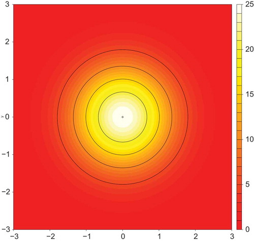
The artificial dataset we employ in this section is generated using the “peak” algorithm in the R package MLBench (Leisch and Dimitriadou 2010). Figure 1 depicts the ground truth from which the data is generated. The data is drawn from a two-dimensional normal distribution centered on the origin and scaled to a maximum height of 25. Points are sampled uniformly from the distribution within a circle of radius three about the origin. To generate a training dataset, we sampled 100 such points. A test set was then generated from further 100 random samples. Each example in the dataset is a tuple of the form $(x,y,z)$ where $z$ is the target to predict.

Figure 1. Contour plot showing a two-dimensional distribution from which artificial data points were sampled. The distribution is defined by the equation $z=25e^{-\frac{1}{2}{r}^2}$ where $r$ is the distance of each sample point $(x,y)$ from the origin.

We note the following points about this artificial regression problem:

1. The target variable $z$ is a non-linear function of the two predictors $x$ and $y$. This property of the data makes the problem difficult for simple linear model learners such as LR. This fact is demonstrated by the performance achieved using the LR algorithm to predict the $z$ values on both the training and test datasets after model learning using the training data: LR achieves a very poor RMSE score of 8.4 on the training data and 8.7 on the test data.

2. The predictive features $x$ and $y$ are not conditionally independent given the predictive target $z$, which violates naive Bayes’ conditional independence assumption. Once $z$ is known, the potential values for $(x,y)$ are distributed around the perimeter of a circle centered on the origin. Thus, knowing the value of $x$ limits the locations for $y$ to two possible values. In contrast to LR, NBR achieves RMSE scores of 1.4 and 2.1 on the two data splits, respectively, which is a major improvement but still not ideal.

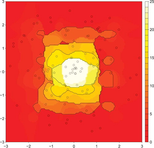
To visualize the model that NBR learns from the training data, we constructed the contour plot depicted in Figure 2. Data from the plot was generated by dividing the $[-3\dots 3]\times [-3\dots 3]$ square centered on the origin into a $120\times 120$ grid. At each grid point, we used the NBR model to make a prediction. Thus, $121\times 121$ predictions were made in total, and the contour plot shows the predicted values. Figure 2 also depicts the 100 randomly sampled training data points used to construct the model as points on the contour plot.

Figure 2. Predicted distribution using the NBR algorithm trained using the 100 training examples. The examples are depicted in the figure as points, and were generated using the R package MLBench (Leisch and Dimitriadou 2010).

Next, we ran the CSO-NBR algorithm 10 times with the same settings as before ($s=100$, $\phi =0.1$, $t_{max}=1000$, $n=10$) and selected the resulting single best artificial training dataset from across the 10 runs. The average model achieved an RMSE of $0.7\pm 0.12$ on the test data. The best model, on the other hand, achieved an RMSE score of 0.4 on the training data and 0.5 on the test data – both the average and best results are a substantial improvement on both LR and standard NBR.

Figure 3 depicts the predictions made by the CSO-NBR model along with the $(x,y)$ coordinates of the ten artificial data points in the best artificial datasets used to build the model. Table 13 further shows the actual artificial data points themselves. We can make several observations from the contour plots of the predictions and the table. Firstly, as Figure 2 clearly shows, the NBR algorithm by itself models the ground truth to a reasonable degree. The predicted $z$ values are higher the closer that $(x,y)$ is to the origin, which is what is expected. However, the circular symmetricity of the distribution in Figure 2 is not preserved well, as the contours have an obvious “squarish” appearance. There also appears to be a high degree of noise in the contours, suggesting that the model is not generalizing well and instead overfitting the training data noise.

Table 13. Artificial data (rounded to 2 d.p.) used to train the model whose predictions are depicted in Figure 3.

$x$	$y$	$z$
1.75	−1.60	0.72
0.08	−0.09	30.89
1.02	−0.94	9.87
0.02	−0.06	−2.81
2.26	−2.15	−5.22
−0.88	0.87	11.73
0.37	−0.48	17.51
1.76	1.82	1.58
−2.06	2.01	−2.91

Figure 3. Predicted distribution using the CSO-NBR algorithm trained using 10 optimized artificial training examples. The examples are depicted in the figure as points.

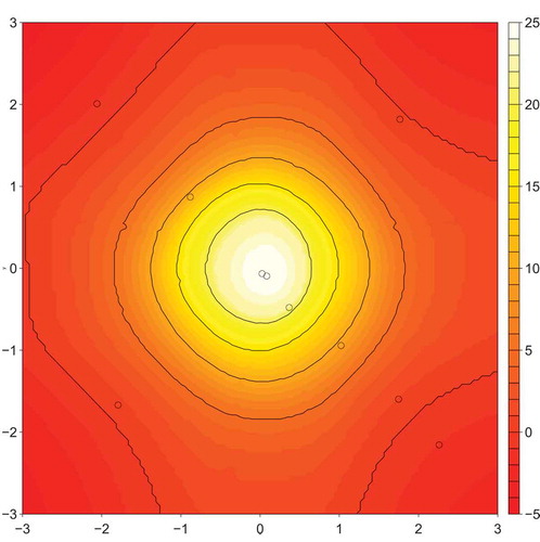
In contrast, the CSO-NBR predictions as depicted in Figure 3 produce a much cleaner, more symmetric, and less noisy predicted distribution. The prediction agrees well with the ground truth distribution in Figure 1, which in turn explains the low RMSE scores achieved in the experiments we performed. Of interest is the layout of the artificial data points across the distribution of predictions. Clearly, the positions of the artificial points have been highly optimized with the majority of the points lying approximately on the negative diagonal $y=-x$ and the remaining two points lying on the opposite diagonal. This configuration of points, when used as training data for the NBR algorithm, produces superior predictions and indicates that only a small amount of training data is required to effectively model this problem.

We additionally performed some time experiments with NBR and CSO-NBR on the artificial data. Over 10 runs on an Intel Core i7-6700K CPU running at 4.00 GHz with 64GB of RAM and using the same settings as above, the mean training time for NBR was 0.017 s, compared to 98.97 s for CSO-NBR. CSO-NBR made use of six cores while our NBR implementation is single-threaded. When we increased the dimensionality of problem from two to ten dimensions (by creating a new artificial dataset with the same number of examples), the mean runtimes of both algorithms were 0.097 s vs. 428.23 s. For the 30-dimensional peak problem, the runtimes were 0.28 s and 1241.99 s.

Clearly, the training time for CSO-NBR is much higher than NBR (which is to be expected, since each run of CSO-NBR builds approximately 500,000 NBR models), and moreover, the training time increases at a rate that is worse than linear with the dimensionality of the regression problem. We expect that the training for CSO-NBR, in practice, would be even worse, since in these experiments we have held the number of iterations constant. With an increase in dimensionality, however, comes a corresponding increase in the size of the search space for CSO, and therefore to properly solve the problem CSO will need significantly more iterations. Mitigating this, however, is the fact that CSO is an “embarrassingly parallel” algorithm: i.e., doubling the number of cores available should effectively halve the runtime.

Conclusion

In summary, we have described a method for enhancing the predictive accuracy of naive Bayes for regression. The approach employs “real” training data only indirectly in the machine learning pipeline, as part of a fitness function that in turn is used to optimize a small artificial surrogate training dataset. The naive Bayes model is constructed using the artificial data instead of the real training data. Our evaluation has demonstrated that the method often produces superior regression models in terms of generalization error.

The primary advantages of this idea are twofold. In its original formulation, naive Bayes typically underperforms other regression models. However, the algorithm does have certain specific advantages such as being simple and interpretable, and interpretable models are important in many areas (e.g., medicine) where understanding the rules used for prediction is important. Finding new methods to enhance the accuracy of naive Bayesian models is therefore important, and we have described one means of doing so.

Several interesting questions are raised by this research, which may form a basis for future work. For example, how hard is this problem when framed as an optimization problem, from a fitness landscape perspective? “Easy” problems in evolutionary computation are usually those with a high correlation between the fitness of solutions and their distance to the global optima. “Hard” problems, on the other hand, have a much lower or even negative (in the case of deception) correlation.

Another question concerns the behavior of our proposed algorithm when a base algorithm quite different to NBR is employed. How exactly does CSO’s behavior change with the base model? Can we replace NBR with a full Bayesian network or a decision tree ensemble and still get generalization improvements? Do we need to use larger or smaller artificial datasets to make our approach work with other base algorithms?

There is also the issue of how to select the optimal artificial dataset size for the problem at hand. Our results indicate that there is no single value of $n$ that is a good default in most cases. Some problems require a larger $n$, and others a smaller $n$. How, then, can the correct $n$ be chosen? A potential but expensive answer to this question is to run the algorithm multiple times with different artificial dataset sizes and attempt to hone in on the best one. However, other more intelligent approaches (for example, greedily adding one optimized example to the artificial dataset at a time until no more improvements are possible) are certainly possible and may work.

Understanding how and why the algorithm works theoretically is a vital next step. Recently, efficient algorithms for computing influence functions have been proposed in the literature (Koh and Liang 2017). Influence functions relate the change in weight of a training example to training loss, and are therefore a means of assessing the impact of each individual example on predictive performance. Are these ideas applicable here? If so, we could use them to understand the relationship between real and fake training data, and model predictions.

Research involving surrogate models for evolutionary algorithms may also yield improvements. If the fitness of a model trained from a dataset can be estimated approximately using a different model, then the optimization speed could potentially speed up significantly. Again, influence functions may be useful other; other surrogate model approaches could also be explored.

Finally, is it possible that useful information might be discovered in these small highly optimized artificial datasets, in the same way that rules and other knowledge can be typically discovered by inspecting normal machine learning models? Figure 3 shows that the optimized artificial data points are uniformly distributed across the space of examples. Would it be possible to take an artificial dataset like this and use a different type of analysis to extract useful knowledge about the problem domain?

Notes

1. Original datasets available from http://prdownloads.sourceforge.net/weka/datasets-numeric.jar.

Appendix A

Table A1. Results of running SPSO and SPSO-NBR on the datasets used in the first experiment with $s=50$ and $t_{max}=1000$.

Dataset	NBR	SPSO-NBR(mean)	SPSO-NBR(best)
Auto93	5.41	7.28 ± 2.53	4.46
AutoHorse	12.92	19.53 ± 2.84	16.56
AutoMpg	3.43	3.56 ± 0.28	3.04
AutoPrice	2375.45	2418.18 ± 217.03	2171.16
Baskball	0.11	0.10 ± 0.01	0.08
Bodyfat	1.68	1.33 ± 1.24	0.70
Bolts	7.92	9.48 ± 2.22	5.82
Cholesterol	61.76	52.80 ± 2.04	49.40
Cleveland	1.05	0.86 ± 0.07	0.79
Cloud	0.43	0.55 ± 0.20	0.37
Cpu	114.65	56.95 ± 32.54	19.48
Detroit	89.18	63.51 ± 21.85	38.91
EchoMonths	12.67	12.20 ± 1.14	10.74
Elusage	17.73	17.84 ± 2.32	14.93
Fishcatch	209.45	80.08 ± 16.97	53.79
Fruitfly	19.80	16.89 ± 0.93	15.40
Gascons	17.63	5.54 ± 2.63	3.04
Housing	6.32	4.53 ± 0.87	3.95
Hungarian	0.36	0.34 ± 0.02	0.32
Longley	552.15	910.21 ± 504.25	408.73
Lowbwt	559.99	479.54 ± 30.36	455.66
Mbagrade	0.30	0.33 ± 0.02	0.31
Meta	378.52	511.75 ± 243.39	184.12
Pbc	1049.74	1026.42 ± 46.36	964.19
Pharynx	354.80	330.98 ± 31.81	303.07
Pollution	62.31	66.89 ± 26.40	43.90
PwLinear	2.49	2.24 ± 0.17	2.04
Quake	0.27	0.20 ± 0.00	0.19
Schlvote	1956688.47	1222473.32 ± 297248.95	1028636.70
Sensory	0.94	0.82 ± 0.02	0.78
Servo	1.04	0.88 ± 0.18	0.67
Sleep	4.09	11.43 ± 20.98	2.43
Strike	696.60	672.86 ± 10.21	656.73
Veteran	164.17	191.26 ± 45.31	145.96
Vineyard	1.33	2.35 ± 0.25	1.91

Shown are the test errors. Bolded figures in the SPSO-NBR(mean) column indicate a better result than the corresponding CSO-NBR(mean) result.

Table A2. Results of running SPSO and SPSO-NBR on the datasets used in the first experiment with $s=100$ and $t_{max}=500$.

Dataset	NBR	SPSO-NBR(mean)	SPSO-NBR(best)
Auto93	5.41	6.58 ± 1.23	5.07
AutoHorse	12.92	17.08 ± 2.74	12.61
AutoMpg	3.43	3.55 ± 0.22	3.19
AutoPrice	2375.45	2524.65 ± 536.17	2217.93
Baskball	0.11	0.10 ± 0.04	0.08
Bodyfat	1.68	0.70 ± 0.10	0.53
Bolts	7.92	9.11 ± 3.41	5.12
Cholesterol	61.76	54.37 ± 2.47	50.80
Cleveland	1.05	0.84 ± 0.08	0.75
Cloud	0.43	0.55 ± 0.16	0.34
Cpu	114.65	77.61 ± 36.68	25.26
Detroit	89.18	45.27 ± 11.89	28.58
EchoMonths	12.67	11.89 ± 0.75	11.25
Elusage	17.73	17.35 ± 2.30	13.38
Fishcatch	209.45	92.72 ± 66.22	55.98
Fruitfly	19.80	18.02 ± 1.25	16.48
Gascons	17.63	5.93 ± 2.48	2.39
Housing	6.32	4.10 ± 0.13	3.92
Hungarian	0.36	0.34 ± 0.02	0.31
Longley	552.15	1061.36 ± 1367.85	372.86
Lowbwt	559.99	522.28 ± 59.45	466.73
Mbagrade	0.30	0.34 ± 0.03	0.32
Meta	378.52	566.25 ± 316.02	97.00
Pbc	1049.74	1009.47 ± 57.85	919.29
Pharynx	354.80	325.70 ± 44.74	272.44
Pollution	62.31	57.13 ± 15.40	44.13
PwLinear	2.49	2.26 ± 0.27	2.01
Quake	0.27	0.20 ± 0.00	0.19
Schlvote	1956688.47	1157391.48 ± 201257.39	1023514.27
Sensory	0.94	0.83 ± 0.02	0.80
Servo	1.04	0.76 ± 0.12	0.60
Sleep	4.09	4.79 ± 3.24	2.55
Strike	696.60	668.92 ± 13.44	655.56
Veteran	164.17	173.83 ± 30.15	140.91
Vineyard	1.33	2.61 ± 0.72	2.11

Shown are the test errors. Bolded figures in the SPSO-NBR(mean) column indicate a better result than the corresponding CSO-NBR(mean) result.

References

- Agrawal, R., T. Imielinski, and A. Swami. 1993. Database mining: A performance perspective. IEEE Transactions on Knowledge and Data Engineering 5 (6):914–25. doi:10.1109/TKDE.69.
- Bonyadi, M., and Z. Michalewicz. 2017. Particle swarm optimization for single objective continuous space problems: A review. Evolutionary Computation 25 (1):1–54. doi:10.1162/EVCO_r_00180.
- Brameier, M., and W. Banzhaf. 2007. Linear genetic programming. Springer US.
- Breiman, L. 1996. Bagging predictors. Machine Learning 24 (2):123–40. doi:10.1007/BF00058655.
- Breiman, L. 2001. Random forests. Machine Learning 45 (1):5–32. doi:10.1023/A:1010933404324.
- Candanedo, L., V. Feldheim, and D. Deramix. 2017. Data driven prediction models of energy use of applicances in a low energy house. Energy and Buildings 140:81–97. doi:10.1016/j.enbuild.2017.01.083.
- Chawla, N., K. Bowyer, L. Hall, and W. Kegelmeyer. 2002. Synthetic minority over-sampling technique. Journal of Artificial Intelligence Research 16:321–57. doi:10.1613/jair.953.
- Cheng, R., and Y. Jin. 2015. A competitive swarm optimizer for large scale optimization. IEEE Transactions on Cybernetics 45 (2):191–204. doi:10.1109/TCYB.2014.2322602.
- Cortez, P., A. Cerdeira, F. Almeida, T. Matos, and J. Reis. 2009. Modeling wine preferences by data mining from physicochemical properties. Decision Support Systems 47 (4):547–53. doi:10.1016/j.dss.2009.05.016.
- Escalante, H., K. Mendoza, M. Graff, and A. Morales-Reyes. 2013. Genetic programming of prototypes for pattern classification, 100–07. Berlin, Heidelberg: Springer Berlin Heidelberg.
- Frank, E., M. Hall, and I. Witten. 2016. The WEKA workbench. Online Appendix for “Data Mining: Practical Machine Learning Tools and Techniques”. Morgan Kaufmann US, 4th edition.
- Frank, E., L. Trigg, G. Holmes, and I. Witten. 2000. Naive Bayes for regression. Machine Learning 41:5–25. doi:10.1023/A:1007670802811.
- Goodfellow, I., J. Pouget-Abadie, M. Mirza, B. Xu, D. Warde-Farley, S. Ozair, A. Courville, and Y. Bengio. 2014. Generative adversarial nets. In Ghahramani Z. et al. (Eds.) Advances in Neural Information Processing (NIPS) 27, pp. 2672-2680, Current Associates Inc.
- Greene, C., D. Hill, and J. Moore. 2009. Environmental noise improves epistasis models of genetic data discovered using a computational evolution system. Proc. GECCO’09, 1785–86, Montreal, Canada.
- Guozhong, A. 1996. The effects of adding noise during backpropagation training on generalisation perfor- mance. Neural Computation 8 (3):643–74. doi:10.1162/neco.1996.8.3.643.
- Impedovo, S., F. Mangini, and D. Barbuzzi. 2014. A novel prototype generation technique for handwriting digit recognition. Pattern Recognition 47 (3):1002–10. doi:10.1016/j.patcog.2013.04.016.
- Kapur, A., K. Marwah, and G. Alterovitz. 2016. Gene expression prediction using low-rank matrix completion. BMC Bioinformatics 17:243. doi:10.1186/s12859-016-1106-6.
- Kennedy, J., R. Eberhart, and Y. Shi. 2001. Swarm intelligence. The Morgan Kaufmann Series in Artificial Intelligence. Morgan Kauffman, US.
- Koh, P. W., and P. Liang. 2017. Understanding black-box predictions via influence functions. In Proceedings of the 34th International Conference on Machine Learning, volume 70 of Proceedings of Machine Learning Research, ed. D. Precup and Y. W. Teh, 1885–94. Sydney, Australia: International Convention Centre, August 06–11. PMLR. http://proceedings.mlr.press/v70/koh17a.html.
- Leisch, F., and E. Dimitriadou. 2010. MLbench: Machine learning benchmark problems, v. 2.1-1 edition.
- Lenz, G., G. Wright, S. S. Dave, W. Xiao, J. Powell, H. Zhao, W. Xu, B. Tan, N. Goldschmidt, J. Iqbal, et al. 2008. Stromal gene signatures in large-b-cell lymphomas. New England Journal of Medicine 359 (22):2313–23. PMID: 19038878. doi:10.1056/NEJMoa0802885.
- Lòpez, V., I. Triguero, C. Carmona, S. Garcia, and F. Herrara. 2014. Addressing imbalanced classification with instance generation techniques: IPADE-ID. Neurocomputing 126 (15–28):15–28. doi:10.1016/j.neucom.2013.01.050.
- Mayo, M., and Q. Sun. 2014. Evolving artificial datasets to improve interpretable classifiers. 2014 IEEE Congress on Evolutionary Computation (CEC), Beijing, China, 2367–74.
- Triguero, I., J. Derrac, S. Garcia, and F. Herrera. 2011. A taxonomy and experimental study on prototype generation for nearest neighbor classification. IEEE Trans. On Systems, Man and Cybernetics – Part C: Applications and Reviews 42 (1):86–100. doi:10.1109/TSMCC.2010.2103939.
- Tsanas, A., M. A. Little, P. E. McSharry, and L. O. Ramig. 2010. Accurate telemonitoring of Parkinson’s disease progression by non-invasive speech tests. IEEE Transactions on Biomedical Engineering 57:884–93. doi:10.1109/TBME.2009.2036000.
- Tsanas, A., and A. Xifara. 2012. Accurate quantitative estimation of energy performance of residential buildings using statistical machine learning tools. Energy and Buildings 49:560–67. doi:10.1016/j.enbuild.2012.03.003.
- Urbanowicz, R., N. Sinnot-Armstrong, and J. Moore. 2011. Random artificial incorporation of noise in a learning classifier system environment. Proc. GECCO’11, 369–74, Helsinki, Finland.
- Vincent, P., H. Larochelle, Y. Bengio, and P. Manzagol. 2008. Extracting and composing robust features with denoising autoencoders. Proc. 25th International Conference on Machine Learning (ICML’08), Helsinki, Finland.
- Wang, Y., and I. Witten. 1997. Induction of model trees for predicting continuous classes. In Poster papers of the 9th European Conference on Machine Learning, Springer, Prague, Czech Republic
- Wang, Z. bujar: Buckly-James regression for survival data with high dimensional covariates. Technical report, 2015. doi:10.1094/PDIS-09-14-0954-PDN.
- Zhong, K., R. Guo, S. Kumar, B. Yan, D. Simcha, and I. Dhillon. 2017. Fast classification with binary prototypes. Proceedings of the 20th International Conference on Artificial Intelligence and Statistics, vol 54, 1255–63, Florida, US. PMLR.