An Analysis of Fast Learning Methods for Classifying Forest Cover Types

ABSTRACT

Proper mapping and classification of Forest cover types are integral in understanding the processes governing the interaction mechanism of the surface with the atmosphere. In the presence of massive satellite and aerial measurements, a proper manual categorization has become a tedious job. In this study, we implement three different modest machine learning classifiers along with three statistical feature selectors to classify different cover types from cartographic variables. Our results showed that, among the chosen classifiers, the standard Random Forest Classifier together with Principal Components performs exceptionally well, not only in overall assessment but across all seven categories. Our results are found to be significantly better than existing studies involving more complex Deep Learning models.

Introduction

Classifying non-urban or nature’s environment has always been in the interest of many, whether they are landowners, foresters, environmental scientists, governments, or land management agencies. The scientific importance of classifying forest cover types involves maintaining or reconstructing pre-settlement vegetation, documenting the change in vegetation, observe the impact of climate on nature, mapping of usable fuel and note the water viability in the soil, among others.

Methods involving land-cover classification requires field studies or land-based remote sensing and are therefore costly, time-consuming, and prone to errors. The advancement of satellite and aerial imagery together with recent developments in the field of machine learning has broadened the scope of research. It has also allowed for fast and reliable ways of classifying large territories (Mahesh 2008; Okori and Obua 2011).

The purpose of this study is to calibrate, analyze, and compare the accuracy of selected machine learning methods for classification of forest cover types, but at the same time comparing the results of this study to other articles targeting the same data. The methods chosen for this purpose are Support Vector Machine (SVM), Naive Bayes’ Classifier (NBC), and the Classification Trees’ (CT) extension Random Forest (RF). We further aim to compare and evaluate these methods while also giving an insight to the differences between them.

Related Work

The problem of classifying forest cover type is not new in agricultural data analysis. It has been previously discussed in various studies and through various domains. However, within the scope of machine learning-based methods, the first study of this sort was done by Blackard and Dean (Blackard and Dean 1999) where the authors compared two techniques (Artificial Neural Network (ANN) and Gaussian Driven Discriminant Analysis (DA)) for predicting forest cover types from cartographic variables. In this study, the predictions produced by the ANN model were evaluated based on how well they corresponded with true cover types (absolute accuracy), and on their relative accuracy compared to predictions made by DA, which is a more conventional statistical model. It has been observed that the overall prediction accuracy for the ANN was obtained at 70.51%, with a 95% confidence interval of 70.26–70.80% while the Linear DA (LDA) model was capable of correctly predicting the cover types with almost 58.38% predictive accuracy.

In several articles, this data has been used as a case study where the idea remained to test the proposed algorithm against the existing ones. In one such study, the authors implement their proposed mixture of Linear SVM (LSVM) algorithm to classify forest cover types (Sug 2010). Here, the whole classification problem was converted into a binary classification problem with emphasis on cover type 2 (spruce/fir), which is the largest cover type, containing 283,301 instances, and covers approximately half the dataset. The algorithm was able to correctly predict 80.0% whether each instance belongs to cover type 2. In another study, the author implemented the bagged CART algorithm for classification and obtained 74.0% predictive accuracy of correct classification (Ridgeway 2002).

More recent attempts for land-cover classification of remote sensing data are methods within the field of deep learning (Chen et al., 2014; Karalas et al. 2015; Längkvist et al. 2016). These methods often involve a complex hierarchical structure that requires a large amount of labeled data to be properly trained and also have many hyperparameters that need to be tuned in order to achieve good results.

Our work deviates from the existing literature in a number of ways. First, we aim to apply well-known classification algorithms that are easy to implement and does not require extensive hyperparameter-tuning. We demonstrate the possibility to achieve an effective prediction accuracy with the use of various variable selection methods. Second, we not only focus on getting the overall classification accuracy of the cover types but also analyze the predictive capabilities for each of the individual cover type to show and discuss how our approaches are capable (or not capable) of dealing with an unbalanced data set.

Material and Methods

This section presents a brief summary of the data and the methods that are used in this work.

Data

The Cover type dataset is used in this work and was obtained from the University of California, Irvine, School of Information and Computer Sciences database.¹ It contains 581,012 observations of cover types from four wilderness areas (Rawah: 29,628 hectares; Comanche Peak: 27,389 hectares; Neota: 3,904 hectares; and Cache la Poudre: 3,817 hectares) located in the Roosevelt National Forest of northern Colorado, with no missing values. The data includes 7 categories of different cover types, which is followed by 12 attributes defined below (Blackard and Dean 1999):

1. The elevation (in meters),

2. The aspect (in degrees azimuth),

3. The slope (in degrees),

4. The horizontal distance to the nearest surface of a water feature in meters (HDTH),

5. The vertical distance to nearest surface water feature in meters (VDTR),

6. The horizontal distance to nearest roadway in meters (HDTR),

7. A relative measure of incident sunlight at 09:00 h on the summer solstice (from a 0-255 index),

8. A relative measure of incident sunlight at noon on the summer solstice (from a 0-255 index),

9. A relative measure of incident sunlight at 15:00 h on the summer solstice (from a 0-255 index),

10. The horizontal distance to nearest historic wildfire ignition point in meters (HDTFP),

11. The soil type designation (40 binary values, one for each soil type)

    and

12. The wilderness area designation (four binary values, one for each wilderness area).

Using Digital Elevation Model (DEM) data from USGS, elevation could be obtained by 30 × 30 m raster cells (in a 1:24,000 scale) Elevation (1) was recorded. By standardizing the DEM data within their 30 × 30 cells, one also obtained Aspect (2), Slope (3) and the three relative measures of sunlight (7–9). Applying the Euclidean distance analyses to the USGS hydrologic and transportation data, one was able to measure the horizontal distance to the nearest water source (4) and roadway (6). The Euclidean analysis was also used on the USFS data, to find the nearest historical wildfire ignition point distance (10), since the last 20 years. To find the nearest vertical distance to a water feature (5), a mix between the DEM, hydrologic data, and a spatial analysis program was used. The USFS database obtained the soil type (11), and the wilderness area designation (12).

As summarized in Table 1, the different forest cover types presented in the data are; 1 lodgepole pine (Pinus contorta), 2 spruce/fir (Picea engelmannii and Abies lasiocarpa), 3 ponderosa pine (Pinus ponderosa), 4 Douglas-fir (Pseudotsuga menziesii), 5 aspen (Populus tremuloides), 6 cottonwood/willow (Populus angustifolia, Populus deltoides, Salix bebbiana and Salix amygdaloides), and 7 krummholz. The krummholz forest cover type class is composed primarily of Engelmann spruce (Picea engelmannii), subalpine fir (Abies lasiocarpa), and Rocky Mountain bristlecone pine (Pinus aristata). Other, minor cover types existed in the areas but were ignored due to their insignificance in regards to their size (Blackard and Dean 1999).

Table 1. Number of observations in each cover type category.

Cover type	Type 1	Type 2	Type 3	Type 4	Type 5	Type 6	Type 7	Overall
Observations	211,840	283,301	35,754	2,747	9,493	17,367	20,510	581,012
Percentage	36.5	48.9	6.15	0.47	1.63	2.99	3.53	100.0

Having 10 continuous variables, 4 wilderness areas and 40 binary soil types, it produced in total 54 different variables available for the used models.

It can be seen from Table 1 that there exists quite a bit of imbalance between the categorical outcomes. This will be kept in consideration when analyzing the results since different methods perform differently depending on how balanced the dataset is. The correlation matrix between the continuous variables is reported in Table 2. Some of the variables are found to be correlated, most notably the variables associated with the relative measure of incident sunlight recorded at different time points shows levels of associations among one another.

Table 2. Table of correlation for the continuous variables. Notable correlations are marked bold.

Variables	1	2	3	4	5	6	7	8	9	10
(1) elevation	1.00
(2) aspect	0.02	1.00
(3) slope	−0.24	0.08	1.00
(4) HDTH	0.31	0.02	−0.01	1.00
(5) VDTR	0.09	0.07	0.28	0.61	1.00
(6) HDTR	0.37	0.03	−0.22	0.07	−0.05	1.00
(7) hillshade9am	0.11	−0.58	−0.33	−0.03	−0.17	0.03	1.00
(8) hillshadenoon	0.21	0.33	−0.53	0.05	−0.11	0.19	0.01	1.00
(9) hillshade3pm	0.06	0.65	−0.18	0.05	0.04	0.11	−0.78	0.59	1.00
(10) HDTFP	0.15	−0.11	−0.19	0.05	−0.07	0.33	0.13	0.06	−0.05	1.00

Methods

The evaluation of the different classification models is going to be based not only on the overall prediction accuracy but also on the accuracy of correctly predicting each of the cover types’ classes. To avoid overfitting to the training data we use k-fold cross-validation technique, which is generally used when estimating how accurate results a method can be assumed to achieve when evaluated on data that is independent of the training data. The overall accuracy was calculated by taking the average of each correctly predicted type divided by the total number of observations of all fivefold cross-validation sets. There are approximately 464,800 observations in the training sets and 116,200 in the test sets.

Learning Algorithms

The most common and relatively simpler machine learning algorithms are used in this article. The goal remains at observing predictive accuracy of these algorithms compared to the more complicated ones, such as deep learning which is computationally expensive and involve huge number of parameters to be estimated and tuned. For our purpose, we rely on known sets of algorithms, which include, the Support Vector Machine (SVM), Naive Bayes’ Classifier (NBC), and Decision Trees (DT). A brief account on the working mechanism of these methods is given in Appendix.

Feature Selection

Besides the choice of algorithms, an equally important aspect is the dimension of the model. The term parsimony refers to when maximum information can be obtained with minimum use of resources. In statistical modeling, it can be translated as finding a simple model with fewer variables that have a high explanatory power. A general aim is to not use more variables in the model than necessary without losing too much information. Most data sets contain a notable amount of variables or attributes and it is therefore essential to find a right combination of variables contributing to better describe the overall structure of the data. Feature selection methods have been developed to extract such useful variables which are necessary to be included in the model. In this work we implemented a number of known feature selection methods, namely, the Random Forest selection, Lasso, and Principal Component Analysis, to find the right combination of the total 54 attributes to be then used in the model, and compared their performances with the respect to prediction accuracy.

Results

Evaluation of Variable Selection

This section summarizes the findings when the variable selection methods are implemented to the data. To assess the performance of Random Forest for variable selection, we obtain the Variable Importance (VI) factor presented in Figure 1. A general criterion is to exclude variables which are deemed to have the lowest VI. The rule of thumb, however, is to remove variables having an importance proportion under 5%, but since we only have 12 variables (or 54 attributes, due to categorical variables), excluding 5 (VI below 5%) out of 12 variables might not be a good choice. Therefore, we set our own criterion to exclude the variables that has the smallest VI value out of all the variables, which in our case is the slope variable. Therefore, we build a model without incorporating the slope variable as per suggested by the RF.

Figure 1. A bar plot over the proportional variable importances for Random Forest Variable selection in the same order as Section 2.1.

The Lasso proposed a different set of variables against each of the seven categorical outcomes. The result yielded the exclusion of the variables HDTR and HDTFP while keeping the rest.

While using a Principal Component Analysis as a method for feature selection, there is no clear answer to where the cutoff of the variance proportion should be made. However, taking into consideration the number of principal components (PC) being 54, where quite a bit of them contribute insignificantly to the proportional variance (see Figure 2). We decide to put the threshold at 80% of the proportional variance, which led us to select the first 33 principal components.

Figure 2. A cumulative plot of the proportion of the variance for the variables each PCA component explain.

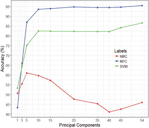
A sensitivity analysis for the PCA accuracy can be seen in Figure 3, it shows evidence of supporting the theory of the NB classifier depends too much on independence to perform well with the PCA for this data. The SVM seems to get approximately a accuracy increase going from of the variance to , but it still does not come close to its full model’s accuracy. However, for the RF based model, the classifier managed to get almost 85% accuracy with only 5 PCAs, which further increased almost upto 95% with 25 PCAs and remained more or less constant when additional components are added to the model.

Figure 3. A plot of the overall accuracy based on the number of principal components included for the Naive Bayes, Random Forest and SVM classifiers (best seen in color).

Here it should be mentioned that a basic Stepwise forward-backward variable selection for multinomial logistic regression is also performed with the Akaike information criterion (AIC) as a decisive criterion (Menard 2002). However, the most optimal AIC value is obtained for the full model. Since we already include the full model with all the variables in our analysis, the Stepwise variable selection model will not be in focus, but rather indirectly referred to when referring to the full model.

Prediction Accuracy

The accuracy for type is calculated as where is the correct number of predictions for type and is the total number of predictions for type . The average overall classification accuracy and the per-class accuracy from a 5-fold cross-validation for the three models and different methods for variable selection can be seen in Table 3.

Table 3. Overall and forest type accuracy for all three methods, the standard deviation of the cross-validation is given in the parenthesis.

	Overall	Type 1	Type 2	Type 3	Type 4	Type 5	Type 6	Type 7
SVM
	89.0	85.4	92.4	91.0	84.9	67.3	79.9	82.5
Full model	(0.10)	(0.12)	(0.13)	(0.33)	(1.43)	(0.72)	(0.50)	(0.50)
	81.8	87.1	88.6	76.5	74.9	10.0	62.9	60.4
Lasso	(0.07)	(0.11)	(0.13)	(0.50)	(1.56)	(1.05)	(0.58)	(1.18)
	89.1	85.5	92.5	91.3	85.0	67.4	80.2	92.7
RF selection	(0.12)	(0.11)	(0.19)	(0.24)	(1.43)	(0.59)	(0.66)	(0.39)
	82.1	77.2	88.4	87.3	70.4	30.2	58.4	83.4
PCA (33)^4	(0.21)	(0.33)	(0.21)	(0.36)	(1.58)	(0.58)	(0.67)	(0.83)
NBC
	66.1	67.5	69.0	78.4	39.0	21.3	30.8	45.1
Full model	(0.09)	(0.19)	(0.11)	(0.38)	(1.27)	(0.86)	(0.47)	(0.75)
	66.8	66.6	72.1	71.5	35.4	15.7	31.0	43.9
Lasso	(0.11)	(0.21)	(0.09)	(0.35)	(1.47)	(0.93)	(0.36)	(0.71)
	66.6	67.7	69.8	78.9	39.1	19.8	29.2	45.7
RF selection	(0.10)	(0.15)	(0.08)	(0.27)	(1.68)	(0.85)	(0.27)	(0.78)
	48.0	78.9	25.5	45.9	69.5	9.9	23.3	79.2
PCA (33)^1	(0.12)	(0.20)	(0.30)	(0.63)	(2.71)	(1.36)	(1.55)	(0.29)
RFC
	84.6	87.1	89.1	80.0	76.9	11.8	63.4	58.9
Full model	(0.23)	(0.34)	(0.29)	(1.00)	(4.46)	(3.06)	(1.35)	(2.64)
	75.2	78.9	80.6	71.2	45.2	0.46	32.7	45.4
Lasso	(0.07)	(0.35)	(0.29)	(2.10)	(2.02)	(0.47)	(1.72)	(1.45)
	84.2	87.1	88.6	76.5	74.9	10.0	62.9	60.4
RF selection	(0.38)	(0.52)	(0.31)	(2.03)	(3.37)	(2.51)	(1.64)	(2.93)
	94.7	93.7	96.7	95.0	77.9	77.0	86.0	94.5
PCA (33)^1	(0.13)	(0.16)	(0.15)	(0.40)	(1.48)	(1.12)	(0.51)	(0.34)
	93.6	92.6	95.9	93.8	75.4	73.7	82.1	93.4
PCA (10)^4	(0.11)	(0.23)	(0.11)	(0.39)	(1.89)	(0.70)	(0.64)	(0.12)

1. PCA made on 33 components out of the total of 54 components.

2. PCA made on 10 components out of the total of 54 components.

Support Vector Machine

Classification accuracies produced by each model as calculated from the test data set are reported in this section. As shown in the first panel of Table 3, when the full model is involved in the learning mechanism, the SVM produced an overall classification accuracy of 89%. When assessing the model strength at predicting individual cover type, the accuracies remained more than or at around 80% for all the cover types except for cover type 5.

When the variables are selected via various methods and then implemented under the SVM, the results show a slightly different picture. For example, with the Lasso variable selection method and SVM model, the overall prediction accuracy decreased a bit from 89% to about 82% for the full model. Here, the prediction accuracy of individual cover type deteriorated to a reasonable amount, most notable for cover type 5, where the model only managed to provide 10% accuracy.

However, when the slope variable is excluded as suggested by the Random Forest variable importance measure, the overall accuracy remained much closer to the case when the full model is used in the learning mechanism (89.1%). similar is the case for the individual cover type prediction, for cover type 7, the model performed much better than the full model with 92.7%.

In the end of the first panel, the results are reported when the PCs are implemented with the SVM. It can be seen that this model managed to get the overall prediction accuracy quite close to the other model (82.1%). However, the accuracies while predicting individual cover types are not very satisfactory.

Naive Bayes

In the second panel of Table 3, we present the predictive accuracies of the Naive Bayes classifier. From a computational perspective, NB is the fastest of these three methods, however, the prediction accuracies are far from being satisfactory. Involving all the variables in the model, the classifier managed to correctly classify the overall cover type for only 66% of the instances (on average). For individual cover types, the performance is not much different which has even deteriorated further for some of the cover types (e.g., 21.3% for type 5). With the model involving variables via the Lasso and the RF, the results are not much different than the Full model case. However, when the model involving principal components, the NB classifier performed the worst in most of the instances, only exceptions are Types 1,4 and 7. The classifier showed evidence of performing worse when classifying the Types 4, 5, 6, and 7 compared to the other 3 cover types. Indicating its limitation on imbalanced data.

Random Forest Classifier

In the last panel of Table 3, we present the results for the Random Forest classifier (RFC). For the full model case, when all the original variables are incorporated, the classifier managed to correctly predict the overall cover type with an accuracy of 84.6%. For the individual case, the results are mixed, where the predictive ability for Types 5, 6, and 7 are not very satisfactory. With Lasso and RF selector suggested variables, the pattern of results is mostly the same. However, using the first 33 PCs in the model, the classifier managed to correctly predict the overall prediction with 94.7%² accuracy, the highest overall accuracy among all combinations. It is noteworthy that, not only for the overall classification, the same model is found to predict individual cover types with highest accuracies. If we recall from Table 2, the association between some of the variables are taken care of when principal components are called upon – this could be one of the reasons as to why the model with PCs is found to be the best.

To further assess the performance of this model, we construct the classification distribution in terms of a confusion matrix and summarized these findings in Table 4. In general, the predictive accuracy is satisfying, even though at some occasions couldn’t correctly classify some instances. The most notable misclassifications are observed when the instances belonging to Type 5 and misclassified as Type 2 (almost 20% of the instances) and Type 4 got misclassified as Type 3 (almost 16.5% of the instances). The next such occurrence appears when the model misclassified almost 6% of the instances with Type 1 where it truly belonged to Type 1. Even though the model misjudged some of the instances wrongly, the overall performance is worth considering and is found to be significantly better than both the models used in this article and existing literature.

Table 4. Confusion matrix for the true (T) and predicted (P) observations from the RFC model with PCA (33), row percentage in the parenthesis and the correct predictions are diagonally in the table.

T\P	1	2	3	4	5	6	7	Sum
1	198,501	12,554	14	0	89	43	639	211,840
	(93.7)	(5.9)	(0.0)	(0.0)	(0.0)	(0.0)	(0.3)	(100.0)
2	7,735	273,905	678	1	437	456	89	283,301
	(2.7)	(96.7)	(0.2)	(0.0)	(0.2)	(0.2)	(0.0)	(100.0)
3	6	596	33,969	166	34	983	0	35,754
	(0.0)	(1.7)	(95.0)	(0.5)	(0.1)	(2.7)	(0.0)	(100.0)
4	0	1	454	2,140	0	152	0	2,747
	(0.0)	(0.0)	(16.5)	(77.9)	(0.0)	(5.5)	(0.0)	(100.0)
5	159	1,858	117	0	7,309	50	0	9,493
	(1.7)	(19.6)	(1.2)	(0.0)	(77.0)	(0.5)	(0.0)	(100.0)
6	18	676	1,621	87	21	14,944	0	17,367
	(0.1)	(3.9)	(9.3)	(0.5)	(0.1)	(86.0)	(0.0)	(100.0)
7	970	147	0	0	2	0	19,391	20,510
	(4.7)	(0.7)	(0.0)	(0.0)	(0.0)	(0.0)	(94.5)	(100.0)
Sum	207,389	289,737	36,853	2,394	7,892	16,628	20,119	581,012
	(35.7)	(49.9)	(6.3)	(0.4)	(1.4)	(2.9)	(3.5)	(100.0)

Discussion

The PCA variable selection method together with the Random Forest classifier gave the highest overall accuracy on this data set. The Naive Bayes Classifier performed worse than the Support Vector Machine and Random Forest Classifier. With this data it might be hesitant to use it, due to the NB’s naive assumption of the predictors being independent, which is doubtful when e.g. three of the variables are the shade index of different times of the day on the same spot. Even though the NB model was trained significantly faster than both the RFC and SVM, it did not make up for its low prediction accuracy.

For this data, the recommended model is the Random Forest Classifier with Principal Component Analysis, since it had a higher accuracy in every way compared to all other tested methods and feature selections and also trained its models notably faster than the SVM’s. On the second place is the SVM Classifier – with a significant increase in time compared to the RFC.

Since one focus was to achieve as high accuracy as possible, a Random Forest classifier with the full PCA selection from a fivefold cross-validation was applied and yielded an accuracy of . Of the previously mentioned studies using this dataset, this is now the highest achieved accuracy. Even using as few components as 10 for the RFC gave still an overall accuracy of , which is still notably higher than the previously mentioned studies where some used the more complex Deep Learning algorithms. Reducing the variance of the PCA from to less than made the RFC loses only in overall accuracy.

The Lasso variable selection method did perform worse in both the Random Forest classifier and Support Vector Machine models, the Naive Bayes model performed slightly better with the Lasso selection model. An explanation might be the correlation or dependence between the variables, see Table 2. The Lasso selection forces itself to select between a group of independent variables that has a high correlation between each other, even if both of those variables might be needed to explain different variations in the data. This might also explain why the NB method did not get as heavily affected by the Lasso method as the RFC and SVM, due to that the NB has the assumption of independence between the predictors.

The Random Forest variable selection performed well with the purpose of a variable (feature) selection. For all three of the methods, it had a rather unchanged accuracy while managing to exclude a predictor, making the time it took to train the model slightly decline. The attractive attribute of Random Forest selection that makes it less sensitive to extreme values was not particularly important here since this data lacked of such values – although, the other attribute of the Random Forest being hard to overfit likely played a big part.

The PCA differed a bit from the Lasso and RF selection. The Lasso and RF selection gave a recommendation of which variables to exclude based on their criteria, but the PCA reworks the variables to principal components by weights (loadings) on each of them, depending on their importance. It then allows one to exclude the components based of their proportion of the explained variance (as could be seen in Figure 2). While one might think that the NB classifier would perform better due to the PCA making the used attributes uncorrelated, it does not necessarily mean that they are independent, rather the PCA method in this case distorted the accuracy for the NB method.

The SVM classifier did not seem to go well with the PCA, either. One reason might be that the SVM kernel computation is not feature wise. PCA reduces the dimensional space, but the SVM does not necessarily need its dimensional space reduced, it is also a risk of the PCA missing out important attributes by transferring the variables into components.

Conclusion

This study assesses the useful of three common machine learning algorithms together with different variable selection methods in accurately classifying the forest cover types. The SVM, NB, and Random forest algorithms are used for classification accompanied by various feature selection methods. It has been observed that the Random Forest classifier provides better accuracy compared to the other set of choices both for the overall assessment and for individual cover types. It highlights the strength of RF algorithm even in accounting for un-balanced data. We noticed that how the prediction accuracy for the random forest classifier together with the PCA managed to achieve a higher accuracy compared to earlier studies where more complex deep learning algorithms like the ANN, only managed to achieve an overall classification accuracy of 70.58%. This shows more support for the theory that feature selection methods should not only be used to reduce the dimensionality of the data but can also to drastically improve the prediction accuracy.

Interesting insight has been noticed when these algorithms are implemented with various feature selection methods. Most particularly, the increase in overall accuracy was not considerable for the SVM (89.0%) or the NB () classifiers when a feature selection method was used compared to the case when all the attributes are used in model fitting. However, when a dimension reduction method, PCA (with 33 components), is coupled with the Random Forest classifier, the overall accuracy jumped from to , which, to our knowledge, is the highest achieved accuracy for the chosen data set.

The classification accuracy achieved with the Random Forest classifier together with the full principal components obtained in this study supersedes other results obtained from previous studies. These findings suggest that the algorithm can be a viable alternative to traditional approaches for classifying forests. With constant changing environment, vegetation, forest fire hazards, and other relevant areas importance, such an algorithm can be a valuable tool in understanding our forests and therefore, assist us in better decision-making and documentation of our nature.

7.1. Support Vector Machine

The Support Vector Machine (SVM) is a supervised machine learning algorithm which is used on a training set and then evaluated with a held-out prediction (or test) set. The input data consist of a set of input vectors () with different features (or attributes) for every observation (or input vector) . Each observation is marked with a label/category that is denoted as . For simplicity, the remaining text denotes the input vector as and the label as for observation . The SVM is primarily a binary learning algorithm with two classes but can be extended for multi-class problems.

7.1.1. Binary Support Vector Model

The SVM learning mechanism aims at finding a directed hyperplane, oriented in such a way that the and are graphically divided by a line into two categories on the hyperplane. The hyperplane (H) that is maximally the most distant from the two input classes is the directed hyperplane and the points closest to the separating hyperplane set up the so-called support vectors. The denotes the separating hyperplane, where is the inner or scalar product, is the offset or bias from the origin in the input space to the hyperplane, and x are the points located within the hyperplane. The weights (W) which are normal to the hyperplane determines its orientation.

Binary SVM classification is popular due to its ability in handling the upper bound of the generalization error instead of local training error, that is standard method in another machine of habitual learning methodologies (Vapnik and Vapnik, 1998). The two important features of such an error are the following:

Feature 1 The bound is minimized by maximizing the margin, where by margin we mean the minimal distance between the hyperplane which separates the two classes and the data-points closest to the hyperplane.

Feature 2 An extra flexibility is added by the fact that, the bound does not depend on the dimensionality of the space.

For binary classifier with data points with corresponding labels , the decision function is:

(1)

More explicitly, the hyperplanes passing through and are called canonical hyperplanes (CH) - we define margin band as the region between these canonical hyperplanes.

Maximizing the margin is equivalent to minimizing:

(2)

which can be reduced to minimizing the Lagrange function consisting of the sum of the objective function and the constraints multiplied by their respective Lagrange multiplier as,

(3)

with are the Lagrange multipliers. Taking the derivatives with respect to and and setting them to zero, lead us to obtain the dual formulation (a.k.a. the Wolfe dual wolfe, 1961). After some simple algebra, we get:

(4)

In equation (4)(4) , we notice that data points only appear inside an inner product. Since we know that the generalized error bound does not depend of dimensionality (see Feature 2), we define an alternative representation of data by mapping into a space with a different dimensionality, the feature space, by replacing

(5)

Here is defined as the mapping function. With the mapping function one is now able to control for both linearly separable and non-linearly separable data. The functional form of is implicitly defined by the choice of kernel: .

In this study, we use the RBF kernel function, which is expressed as

(6)

where is the Gaussian kernel parameter. Knowing the choice of kernel, the learning task for binary classification now involves the maximization of:

(7)

The bias would now look like, considering the cases with and ,

(8)

Finally to construct an SVM binary classifier, we place the data points into equation (7)(7) and maximize, subject to the given constraints. The bias term presented in equation (8)(8) can then be calculated from the optimal values of .

7.1.2. Multi-class Support Vector Model

There are a few ways to extend the binary classification theory to a multi-class SVM. The idea is to decomposes the multi-class problem into a predefined set of binary problems. One such method is the One-Versus-Rest (1VR, a.k.a. One-Versus-All) approach, in which one constructs k separate binary classifiers for a response variable of k categories. Following the notation presented in the previous subsection, define the m-th classifier as a positive and the rest k-1 as negative outcomes. During test, the class label is determined by the binary classifier that gives maximum output value (Ma and Guo 2014). A major problem, however, with the 1VR approach is the imbalanced training set. For equally sized training examples, one classifies one category at a time to be positive, means that the ratio of positive to negative examples is , with an additional cost of loosing symmetry in the original structure.

Another approach referred to as the One-Versus-One approach (1V1) or the pairwise decomposition (Kreßel 1999). It evaluates all possible pair classifiers against each observation and thus, yields individual binary classifiers. Note that, the size of classifiers in 1V1 approach is much larger than that of the 1VR approach. However, the size of lagrange function in each classifier is smaller, which makes it possible to train fast. It can be deduced that the 1V1 approach is considerably more symmetric than the 1VR approach, taking the 1VR’s imbalance weakness into consideration. However, a negative aspect of the 1V1 approach is that it is computationally expensive compared to the 1VR. In this study, since the accuracy has given a higher priority than computational speed, therefore, the the One-Versus-One approach is for Multi-class SVM prediction.

7.2. Naive Bayes’ Classifier

The peculiar name of Naive Bayes’ Classifier origins from the fact that the method assumes the attributes, given their category value, to be independent from each other. This might seems a rather restrictive assumption but saves considerable computational time.

Consider the class with number of categories - the vector is the same as considered in the earlier subsection. The joint probability distribution with the prior probability and the class probability , can now be obtained through that.

Recalling Bayes’ theorem, we get;

(9)

Considering the fact of independence among attributes, equation (9)(9) can be written as,

(10)

The likelihood is usually modeled by using the same class of probability distribution, i.e., binomial or Gaussian. The chosen likelihood distribution in this study is the Gaussian distribution with the class proportions of the training sets as the prior probabilities/distributions.

The choice of output category itself is fairly simple. Assume two different categories and , with be the chosen category if:

(11)

The general notation for the chosen category for () number of categories can be summarized as:

(12)

Where is the estimated output category for the vectors/features .

7.3. Decision Trees

Decision Trees are used both for regression and classification problems. The choice between these two entities is driven by the type of data used to construct such trees. Our focus remains on the Classification trees, since the response variables in the considered data are of qualitative nature.

The basic principle of the CT is to “predict that each observation belongs to the most commonly occurring class of training observation in the region to which it belongs” (James et al. 2014). To make a Classification Tree grow, one uses recursive binary splitting by selecting the predictor and the cutpoint and then splits the tree so that the classification error rate (CER) is given the most possible reduction in the regions and . The CER is just the part of the training observations in that region that do not belong to the most common/predicted class.

Consider all predictors and all possible values for such that the lower tree has the smallest possible CER. Further, assume that the predictor space (i.e. ) are divided into distinct and non-overlapping regions. So, for the case of only and regions, the pair of half-planes for any and are defined as;

(13)

The CER is:

(14)

where is the proportion of the training data in the th region that are from the th class. Since the CER is not very sensitive for tree-growing, another preferred measure is the Gini index (GI), defined as;

(15)

The Gini index (GI) is a measurement of the total variance across the classes. From the equation ((15)), it is rather obvious that the GI takes on a small value if all the proportion, , are close to zero or one. Due to this fact, the GI is referred to as a measurement of node purity, a value which indicates that a node holds most observations from a single class.

In order to improve the prediction accuracy of Decision Trees, several extensions are usually preferred to apply. One such extension, dominated in the existing literatures, is the Random forest based classification (James et al. 2014).

The random forest builds a number of decision trees on bootstrapped training samples. While building such decision trees, each time a split in a tree is considered, a random sample of predictors from the full set of predictors is chosen as split candidates. This split is further restricted to use only one of those predictors. After each split a new sample of predictors are taken, however, the method is not allowed to consider majority of available predictors. One roughly chooses, predictors among the set of all.

Disclosure Statement

No potential conflict of interest was reported by the authors.

Notes

1. https://archive.ics.uci.edu/ml/index.php.

2. 95.4% when using all PCs – although no significant increase, results can be provided upon request.

7. Appendix;

Theory & models

In this section, we summarize the theoretical details of the chosen methods, namely the Support Vector Machine, Naive Bayes’ Classifier, and Decision Trees – Random Forest.

References

- Blackard, J. A., and D. J. Dean. 1999. Comparative accuracies of artificial neural networks and discriminant analysis in predicting forest cover types from cartographic variables. Computers and Electronics in Agriculture 24 (3):131–51. doi:10.1016/S0168-1699(99)00046-0.
- Chen, Y., Z. Lin, X. Zhao, G. Wang, and Y. Gu. 2014. Deep learning-based classification of hyperspectral data. IEEE Journal of Selected Topics in Applied Earth Observations and Remote Sensing 7 (6):2094–107. doi:10.1109/JSTARS.2014.2329330.
- James, G., D. Witten, T. Hastie, and R. Tibshirani. 2014. An introduction to statistical learning: With applications in R. New York: Springer-Verlag.
- Karalas, K., G. Tsagkatakis, M. Zervakis, and P. Tsakalides. 2015. Deep learning for multi-label land cover classification. ‘Image and Signal Processing for Remote Sensing XXI’ 9643 (SPIE):244–57.
- Kreßel, U. H. G. 1999. Pairwise classification and support vector machines. In advances in kernel methods edn, 255–268. Cambridge, MA: MIT Press.
- Längkvist, M., A. Kiselev, M. Alirezaie, and A. Loutfi. 2016. Classification and segmentation of satellite orthoimagery using convolutional neural networks. Remote Sensing 8 (4):329. doi:10.3390/rs8040329.
- Ma, Y., and G. Guo. 2014. Support vector machines applications. SpringerLink: Bücher, Springer International Publishing, Switzerland.
- Mahesh, P. 2008. Artificial immune-based supervised classifier for land-cover classification. International Journal of Remote Sensing 29 (8):2273–91. doi:10.1080/01431160701408402.
- Menard, S. 2002. Applied logistic regression analysis, Vol. 106 of quantitative applications in the social sciences, Sage University Papers Series on Quantitative Applications in the Social Sciences (series no. 07-106). Thousand Oaks, CA: Sage.
- Okori, W., and J. Obua. 2011. Supervised learning algorithms for famine prediction. Applied Artificial Intelligence 25 (9):822–35. doi:10.1080/08839514.2011.611930.
- Ridgeway, G. 2002. Looking for lumps: Boosting and bagging for density estimation. Computational Statistics & Data Analysis 38 (4):379–92. doi:10.1016/S0167-9473(01)00066-4.
- Sug, H. 2010. The effect of training set size for the performance of neural networks of classification. WSEAS Trans Comput 9:1297–306.
- Wolfe, P. 1961. A duality theorem for non-linear programming. Quarterly of Applied Mathematics 19 (3):239–44. doi:10.1090/qam/135625.