Moving Medical Image Analysis to GPU Embedded Systems: Application to Brain Tumor Segmentation

ABSTRACT

With the growth of medical data stored as bases for researches and diagnosis tasks, healthcare providers are in need of automatic processing methods to make accurate and fast image analysis such as segmentation or restoration. Most of the existing solutions to deal with these tasks are based on Deep Learning methods that require the use of powerful dedicated hardware to be executed and address a power consumption problem that is not compatible with the aforementioned requests. There is thus a demand in the development of low-cost image analysis systems with increased performances. In this work, we address this problem by proposing a fully-automatic brain tumor segmentation method based on a Convolutional Neural Network, executed by a low-cost, Deep Learning ready GPU embedded platform. We validated our approach using the BRaTS 2015 dataset to segment brain tumors and proved that an artificial neural network can be trained and used in the medical field with limited resources by redefining some of its inner operations.

Introduction

The development of brain tumor segmentation tools based on Deep Learning (DL) methods has grown significantly over the last few years. Several models like the InputCascadeCNN (Havaei et al. 2017) or the U-Net (Dong et al. 2017) have already shown that great potential lies in the use of Convolutional Neural Networks (CNNs) to help the detection of common tumors that are yet difficult to segment due to the variety of their shapes and locations. With the architectures of these models getting deeper over the years in a rush for performances, a need for powerful platforms appeared to handle their execution leading to the use of more power, resulting in high costs. To fulfill their promises on the production level and be accessible, DL based methods for medical image analysis must be able to be trained and executed on platforms with limited computational resources (Qiu et al. 2016). Moreover, the constant increase of medical data pushes healthcare providers to seek for fullyautomatic image analysis methods in order to offer faster and better diagnoses.

Hence, DL based solutions to computer vision tasks must succeed in affordability, energy-efficiency and portability to be fully considered as real and applicable solutions. The Low-Power Image Recognition Challenge (LPIRC) (Alyamkin et al. 2018) appeared to emphasize the need to develop such systems with a balance between performance and low power consumption as a mean to highlight their importance. In this dynamic, low-power hardware accelerators for DL were developed and launched by several technology companies. The Nvidia Jetson AGX Xavier (JAX) (Pujol et al. 2019) is one of these accelerators built for machine learning that ease the development and deployment of DL applications. Its CPU-GPU architecture supported by CUDA, cuDNN and the TensoRT software libraries for inference speed up makes it the perfect fit to run DL workloads in different domains such as logistics, service, manufacturing, smart city applications and medical image analysis.

In this paper, we first discuss the advantages of the JAX to develop and run DL applications. We then review the use of model compression methods as well as a normalization scheme for the optimization of neural networks in order to allow their deployment on limited resource devices. Finally, we propose a training scheme of a compressed neural network architecture to build an end-to-end automatic brain tumor segmentation tool applied to glioma tumors.

Materials and Methods

The appearance of embedded computing systems gave rise to the development of IoT devices for healthcare (Dang et al. 2019), autonomous cars (Tian et al. 2018), and drones (Tanwani et al. 2007), all taking advantage of power efficiency and portability. The challenge in the development of dedicated machine learning applications executable on this kind of systems followed this growth and still has to be addressed because of the computational complexity of most common algorithms. Designing lightweight DL applications compatible with imposed memory constraints thus demands to rethink and modify some operations to reduce the number of parameters that they involve.

This section studies the efficiency of the JAX as well as modifications of neural network operations for the development of lightweight CNNs.

Jetson AGX Xavier

The unique features of the JAX made it one of the most popular low-cost machine learning accelerator available today. The motivation for using it as a platform to develop and run end-to-end DL applications lays in the will to take advantage of the power provided by its CPU-GPU architecture over the use of FPGAs (Mittal and Vetter 2014) as well as its low weight and low power consumption.

GPU based embedded computing systems like the JAX can thus be a good choice for both training and inference of Deep Learning models in real-time applications for several reasons. The first reason concerns the low weight feature of the platform that is compatible with deployment requirements for small or flying devices since the power required to hover a drone, for example, increases with its mass (Tijtgat et al. 2017). The low power consumption is the second reason as it reduces thermal problems that are inherent to domains like autonomous driving and aims to reduce energy costs. As shown in Table 1, both power consumption and weight features of the JAX are suitable for embedded applications development.

Table 1. Nvidia Jetson AGX Xavier specifications.

	Jetson AGX Xavier Module
CPU	8-core ARM v8.2 64-bit CPU, 8MB L2 + 4MB L3
GPU	512-core Volta GPU with Tensor Cores
Memory	16GB 256-Bit LPDDR4x | 137GB/s
Weight	630 grams
Dimension	100 mm x 87 mm x 16 mm
Storage	32GB eMMC 5.1

The kit also embeds a modular scalable architecture, shown in Figure 1, known as the Deep Learning Accelerator (DLA) and designed to ease the integration and deployment of DL applications while optimizing energy efficiency. This architecture includes a support for most layers used in CNNs, like convolution and deconvolution layers, pooling layers, fully-connected layers, normalization layers and activation layers. This support makes the JAX a great choice for developing CNN based image analysis tools.

Figure 1. The Nvidia deep learning accelerator architecture. Nvdla.org.

One other reason comes from the fact that the kit is ready to receive an NVMe SSD drive to increase its memory and allow to store and process data locally while many real-time DL applications involve the use of remote servers for this same task. Gathering and processing data locally offers the advantage of not relying on a server response that can imply high latency, connection disruptions and possible security flaws when requesting or writing data.

The JAX also embeds the JetPack SDK that includes TensorRT, a high performance deep learning inference runtime that aims to reduce the memory footprint for convolutional neural networks and speeds up inference for image segmentation tasks like the one we address in this paper.

All the mentioned reasons for using the JAX as a training and inference platform for CNNs then motivate the transformation of existing neural network architectures to build smaller and faster models executable with limited power by compressing their building blocks and find new regularization schemes to make sure that these models do not suffer from the reduction of parameters.

Normalization

Normalization methods are known for their capacity to fasten training (LeCun et al. 1998) and have been widely used in deep learning. The most well-known normalization method used to train Deep Neural Networks (DNNs) is called Batch Normalization (Ioffe and Szegedy 2015) (BN). BN has proven to be a very efficient normalization solution to ease neural networks optimization and convergence by performing a global feature normalization along the batch dimension. The stochastic uncertainty of the batch statistics also allows to use BN as a powerful regularizer and helps DNNs to avoid overfitting.

However, despite all of the aforementioned advantages of this method, normalizing along the batch dimension requires BN to work with large batch sizes because small mini-batches lead to inaccurate batch statistics estimation and thus increase the model’s error. Since training on an embedded system requires to be able to use a small amount of memory, it is important to use very small input mini-batches and normalize features along another dimension without penalty on the training performances.

Several methods like the Synchronized Batch Normalization (Peng et al. 2018) and Batch Renormalization (Ioffe 2017) have been proposed to get better performances while solving the batch statistics estimation problem when using BN with small mini-batches. However, these methods stay batch dependent and only move the size problem elsewhere or simply solve it by adding computational power according to the mini-batch size.

Group Normalization (GN) (Wu and He 2018) appears to be one normalization solution when working with resource-constrained systems. The general purpose of a GN layer is to divide input channels into groups and apply normalization on the features present in each of these groups. It avoids the batch statistic computation and stays completely independent to the batch dimension. Considering a regular feature normalization, the standard deviation $\sigma$ and the mean $\mu$ are formulated as in Eq. (1)(1) ${\mu }_i=\frac{1}{m}\sum _{k\in S_i}{x}_k,{\sigma }_i=\sqrt{\frac{1}{m}}\sum _{k\in S_i}(x_k-{\mu }_i{)}^2+\epsilon$(1) where $S_i$ is the set of pixels on which the normalization is performed and $m$ is the size of the set being processed. x represents the features being computed and $\epsilon$ is a small constant.

(1) ${\mu }_i=\frac{1}{m}\sum _{k\in S_i}{x}_k,{\sigma }_i=\sqrt{\frac{1}{m}}\sum _{k\in S_i}(x_k-{\mu }_i{)}^2+\epsilon$(1)

Therefore, GN is defined as the computation of $\sigma$ and $\mu$ in a set formulated as follows:

(2) $S_i=k|k_N=i_N,\lfloor \frac{k_C}{C/G}\rfloor =\lfloor \frac{i_C}{C/G}\rfloor$(2)

where $N$ is the batch axis, $G$ the number of groups and $C/G$ the number of channels per group. Note that in Eq. (2(2) $S_i=k|k_N=i_N,\lfloor \frac{k_C}{C/G}\rfloor =\lfloor \frac{i_C}{C/G}\rfloor$(2) ), if $G=1$, a Layer Normalization (Ba, Kiros, and Hinton 2016) is applied and if $G=C$, where $C$ is the number of input channels, an Instance Normalization (Ulyanov, Vedaldi, and Lempitsky 2016) is applied. This method has shown its potential obtaining lower training error values by replacing BN layers in existing models like the ResNet-50 (He et al. 2016). Hence, using GN as a normalization and regularization layer allows DNNs to be trained on smaller batches, fastens training and avoid memory constraints. In this work, we combined GN with Dropout (Srivastava et al. 2014) to create Independent-Component (IC) layers (Chen et al. 2019), as illustrated in Figure 2, that build a regularization scheme by reducing the correlation between pairs of neurons during training.

Figure 2. Modified separable convolution block replacing each of the U-net regular and transposed convolutions.

Model Compression

Convolutional neural networks have proven their efficiency in solving visual tasks like object detection or image segmentation but still suffer from high computation costs when deployed on devices with limited resources. With the appearance of deeper models, CNNs need to be redefined to be trained on these devices and used for inference in real-time applications.

We based our work on the use of the existing U-net architecture and aimed to make it usable for both training and inference on the JAX platform. For this purpose we used model compression to reduce the number of trainable parameters and gain training speed. As a first compression method we redefined the convolutional operations with the use of depthwise separable convolutions (Sifre and Mallat 2014). This type of convolution can factorize standard convolutions by decomposing them into a depthwise convolution followed by a regular convolution with a kernel of 1 × 1 called pointwise convolution as shown in Figure 3. In contrast to regular convolutions, depthwise separable convolutions apply a single filter for each channel in the input independently. Hence, if $K$ is the size of the convolutional kernel, $M$ the number of input channels, $G$ the size of the output image and $N$ the number of output channels, the number of trainable parameters of regular convolutions is set as in Eq. (3)(3) $K^2\cdot M\cdot G^2\cdot N$(3) while the decomposition offered by depthwise separable convolutions sets the number of trainable parameters to Eq. (4)(4) $G^2\cdot M\cdot (K^2+N)$(4) .

(3) $K^2\cdot M\cdot G^2\cdot N$(3)

(4) $G^2\cdot M\cdot (K^2+N)$(4)

Figure 3. Composition of a separable convolution block.

Taking advantage of this compression ability MobileNet (Howard et al. 2017) and ShuffleNet (Zhang et al. 2018) are the most popular models implemented using separable convolutions in order to achieve competitive results in common visual tasks such as ImageNet (Deng et al. 2009). We thus replaced each convolutions in both encoder and decoder part of the U-net architecture by separable convolution blocks similar to the ones used by the MobileNetV2 (Sandler et al. 2018, June) architecture as shown in Figure 4. These blocks are composed of three smaller convolution blocks. The first convolution sub-block is a regular 1 × 1 convolution block, it is followed by a depthwise convolution block and a pointwise convolution block. Only the regular and depthwise convolution sub-blocks are activated by a LeakyReLU function. Each of the sub-blocks uses the IC layer described previously for normalization and regularization. To compress the network even more, we set the number of output maps in the bottleneck of the architecture to 512 and each transposed convolution in the decoder part of the architecture is replaced by an upsampling layer using bilinear interpolation (Pandey, Vasan, and Ramakrishnan 2018; Parker, Kenyon, and Troxel 1983). The entire proposed architecture of the network built with the operations, introduced previously, is illustrated in Figure 4.

Figure 4. Our compressed U-net architecture. It consists of MobileNetV2-like separable convolution blocks coupled with max-pooling for downsampling in the encoding part of the network and bilinear upsampling in the decoding part.

In addition to the compression of the convolution layers, neural network quantization (Migacz 2017; Park, Ahn, and Yoo 2017) was used for inference. Since the operations of DNNs can be clipped down to 8-bit fixed-point without major penalty in the inference performance, we compressed our model even further by using a post-training 8-bit quantization to accelerate the prediction phase of our method and reduce the time needed for segmentation. The advantage of using quantization as a neural network compression method is then twofold, it speeds up inference and offers a solution to the power efficiency problem involved in most DL applications by reducing memory access costs and memory bandwidth (Louizos et al. 2018).

Experiments and Results

Dataset

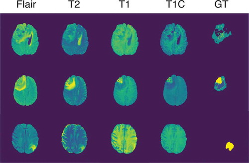
Our experiments were run using the BraTS 2015 (Menze et al. 2015) dataset. The training set includes 220 cases of high-grade glioma (HGG) and 54 cases of low-grade glioma (LGG). For each case, four sequences are available: Flair, T2, T1, and T1 c. Each brain in the set also comes with a ground truth image containing 5 labels corresponding to the tumor structures, namely non-tumor (label 0), necrosis (label 1), edema (label 2), non-enhancing tumor (label 3) and enhancing tumor (label 4). These structures are grouped in 3 regions, the complete tumor region (containing all four labels), the core tumor region (containing all labels except edema) and the enhancing tumor region (only containing the enhancing tumor structure). Figure 5. shows the four sequences in the given order and their associated ground truth from an LGG case on the upper row and two HGG cases on the two bottom rows.

Figure 5. Four sequences and ground truth of an LGG case and two HGG cases taken from the BRaTS 2015 dataset.

Before being processed by the neural network, we first applied some pre-processing operations to the data by applying the N4ITK bias field correction (Tustison et al. 2010) to the T1 and T1 c sequences using the SimpleITK library (Lowekamp et al. 2013). We also randomly applied different data augmentations like elastic transformation, flipping, gaussian noise or shifting to 40% of the slices in order to prevent the model from overfitting.

Since data have to be processed locally on the embedded system, we need to define a fast and light pipeline to feed the neural network. We decided to extract slices from each case by ignoring each empty slice, we cropped each of them to 128 × 128 in order to avoid extra computation over the MRIs background regions. Our pipeline thus creates a training and a validation dataset separately with a split ratio of 0.8/0.2 containing both HGG and LGG cases. Finally, to reduce the dataset size in memory and gain reading speed for later processing, the extracted slices are saved and encoded using a Protocol Buffer format.

Training and Implementation Details

The model was trained using an Adam Optimizer (Kingma and Ba 2014) with a learning rate set to 0.0001. All biases were initialized to zeros and the kernels were initialized using the glorot normal initialization (Glorot and Bengio 2010). To get better performances in terms of pixel-wise accuracy, we used Eq. (7)(7) $CombinedLoss(y,\hat{y})=BCE(y,\hat{y})+DiceLoss(y,\hat{y})$(7) as a combined loss function based on the Binary Cross-Entropy (BCE) computed as in Eq. (5)(5) $BCE(y,\hat{y})=-\frac{1}{N}\sum _{i=1}^N[y_{i}log({\hat{y}}_i)+(1-y_i)log(1-{\hat{y}}_i)]$(5) and the Dice loss functions shown in Eq. (6)(6) $DiceLoss(y,\hat{y})=1-\frac{2\sum y\cdot \hat{y}}{\sum y+\hat{y}}$(6) .

(5) $BCE(y,\hat{y})=-\frac{1}{N}\sum _{i=1}^N[y_{i}log({\hat{y}}_i)+(1-y_i)log(1-{\hat{y}}_i)]$(5)

(6) $DiceLoss(y,\hat{y})=1-\frac{2\sum y\cdot \hat{y}}{\sum y+\hat{y}}$(6)

(7) $CombinedLoss(y,\hat{y})=BCE(y,\hat{y})+DiceLoss(y,\hat{y})$(7)

where $N$ is the number of samples in the dataset, $y$ represents the ground truth labels and $\hat{y}$ the model predictions. Since we dealt with the limitations of Batch Normalization, we allow the model to be trained on small mini-batches of size 2. Early stopping is used to prevent the model from overfitting by monitoring the values of the validation loss during training.

The last layer of the model outputs a pixel-wise probabilistic mask wherein each pixel takes a value in the range [0,1] set by a sigmoid activation function. This mask is then thresholded to recover a prediction mask comprising all 5 sparse labels. Finally, since the JAX comes with built-in DL accelerators and visual accelerators that can be configured with 4 different power envelopes, we chose to use the full potential of the embedded platform during training by setting the configuration to the MAXN mode, allowing the use of every CPU Core and an increased GPU Frequency as stated in Table 2. This configuration led to train the model taking about 20 mins per epoch. Note that each of the modes were tested and were all successful in running both training and inference of our model.

Table 2. Nvidia Jetson AGX Xavier power modes.

	MAXN	10 W	15 W	30W_ALL
CPU Cores	8	2	4	8
CPU Max Freq. (MHz)	1377	520	6700	900
GPU Max Freq. (MHz)	2265.6	1200	1200	1200
Memory Max Freq. (MHz)	2133.6	1066	1333	1600

Results

Using the JAX maximum capacity, our segmentation method was successfully able to be trained and to segment high and low grade gliomas. Moreover, while the uncompressed U-Net model involves more than 31 millions of parameters, our compression scheme reduces this number down to about 2.1 millions without major penalty in its training and inference performances in regards to the parameter reduction factor. This reduction of the model memory footprint allows this method to be deployable on embedded systems or be used as a portable application for medical image analysis.

The Dice coefficient was computed over the validation dataset for each of the tumor region described previously as a proof of similarity between the ground truth and the predicted mask as follows:

(8) $DiceCoef=\frac{2|y\cap \hat{y}|}{|y|+|\hat{y}|}$(8)

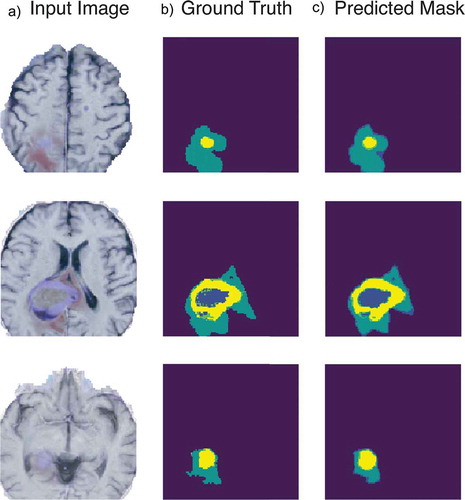
Although other segmentation methods like the ones shown in Table 3 achieve higher dice scores, our method can fairly compare in terms of number of parameters involved to achieve the segmentation task. Figure 6 shows three examples of segmentation achieved by our compressed model where the column A represents the input image as a cropped slice containing all 4 sequences, followed by its ground truth in the B column and the thresholded predicted mask found by the neural network in column C.

Table 3. Results of our proposed approach compared to other similar deep learning based brain tumor segmentation methods.

	Dice Score
Method	Complete	Core	Enhancing
Proposed	0.81	0.77	0.53
Zhao (Zhao et al. 2018)	0.82	0.72	0.62
Pereira (Pereira et al. 2016)	0.84	0.72	0.62
Dong (Dong et al. 2017)	0.86	0.86	0.65

Figure 6. Example of tumor segmentation results. With a 128x128x4 input slice in A, its associated ground truth in B and the compressed model output in C.

Other compression methods could have been used to go further in the reduction of the model footprint, like Knowledge Distillation (Hinton, Vinyals, and Dean 2015) or Parameter Pruning (Suzuki, Horiba, and Sugie 2001). However, we think that such solutions would not be compatible with the development of fast real-time applications for devices with limited resources since they need heavier pre-trained networks to be used, which may not be suitable for the problem stated in this paper since our main interest is to develop and train a DL based segmentation tool without using any prerequisite model.

Conclusion

In this paper, we reviewed some methods used for neural networks optimization and compression and proved that they can successfully be applied to move medical image analysis to limited resources embedded systems. We provided a lightweight neural network training development scheme by integrating model compression in an existing CNN architecture. Using depthwise separable convolutions coupled with Independent-Component layers gives the benefit of reducing the number of trainable parameters without compromising training and inference performances. We compared these performances with other state of the art similar approaches involving the training of Deep Neural Networks and proved that our method can reach comparable results in regards to the reduction of parameters that we applied. We tested the capacity of an affordable embedded platform in the execution of a brain tumor segmentation method and proved that it can be sucessfully used to develop end-to-end Deep Learning based applications for medical image analysis and reduce their cost in production due to the reduction of training and inference time, and the reduction of the general amount of energy used by the system to proceed the segmentation task.

Acknowledgments

This work was supported and partially funded by Région Hauts-de-France, Agglomération du Saint-Quentinois and the city of Saint-Quentin.

References

- Alyamkin, S., M. Ardi, A. Brighton, A. C. Berg, Y. Chen, H.-P. Cheng, … S. Zhuo. 2018. 2018 low-power image recognition challenge. ArXiv, abs/1810.01732.
- Ba, J. L., J. R. Kiros, and G. E. Hinton. 2016. Layer normalization. arXiv preprint arXiv:1607.06450.
- Chen, G., P. Chen, Y. Shi, C.-Y. Hsieh, B. Liao, and S. Zhang. 2019. Rethinking the usage of batch normalization and dropout in the training of deep neural networks. arXiv preprint arXiv:1905.05928.
- Dang, L. M., K. Min, D. Han, M. Jalil Piran, and H. Moon. June 2019. A survey on internet of things and cloud computing for healthcare. Electronics 2019, 8, 768.
- Deng, J., W. Dong, R. Socher, L. Li, L. Kai, and L. Fei-Fei. June 2009. Imagenet: A large- scale hierarchical image database. In 2009 ieee conference on computer vision and pattern recognition, 248–55. Miami, FL. Ieee.
- Dong, H., G. Yang, F. Liu, Y. Mo, and Y. Guo. 2017. Automatic brain tumor detection and segmentation using u-net based fully convolutional networks. Medical Image Understanding and Analysis 506–17. https://doi.10.1007/978-3-319-60964-544
- Glorot, X., and Y. Bengio. 13–15 May 2010. Understanding the difficulty of training deep feedforward neural networks. In Proceedings of the thirteenth international conference on artificial intelligence and statistics, Y. W. Teh and M. Titterington ed., vol. 9, 249–56. Chia Laguna Resort, Sardinia, Italy: PMLR. http://proceedings.mlr.press/v9/glorot10a.html
- Havaei, M., A. Davy, D. Warde-Farley, A. Biard, A. Courville, Y. Bengio, C. Pal, P.-M. Jodoin, and H. Larochelle. January 2017. Brain tumor segmentation with deep neural networks.. Medical Image Analysis 35:18–31. doi: 10.1016/j.media.2016.05.004.
- He, K., X. Zhang, S. Ren, and J. Sun. June 2016. Deep residual learning for image recognition. In Proceedings of the 2016 IEEE conference on computer vision and pattern recognition (CVPR), 770–78. Las Vegas.
- Hinton, G., O. Vinyals, and J. Dean. 2015. Distilling the knowledge in a neural network. arXiv preprint arXiv:1503.02531.
- Howard, A. G., M. Zhu, B. Chen, D. Kalenichenko, W. Wang, T. Weyand, … H. Adam. 2017. Mobilenets: Efficient convolutional neural networks for mobile vision applications. arXiv preprint arXiv:1704.04861
- Ioffe, S. 2017. Batch renormalization: Towards reducing minibatch dependence in batch- normalized models. In Advances in neural information processing systems, 1945–53. Long Beach, USA.
- Ioffe, S., and C. Szegedy. 2015. Batch normalization: Accelerating deep network training by reducing internal covariate shift. In Proceedings of the 32nd international conference on international conference on machine learning - volume 37, 448–56. Lille, France. JMLR.org. http://dl.acm.org/citation.cfm?id=3045118.3045167.
- Kingma, D. P., and J. Ba. 2014. Adam: A method for stochastic optimization. CoRR, abs/1412.6980.
- LeCun, Y., L. Bottou, G. Orr, and K. Muller. 1998. Efficient backprop. In Neural networks: Tricks of the trade, ed. G. Orr and K. Muller, 9-48, Springer, Berlin, Heidelberg. doi:10.1007/978-3-642-35289-83.
- Louizos, C., M. Reisser, T. Blankevoort, E. Gavves, and M. Welling. 2018. Relaxed quantization for discretized neural networks. ArXiv, abs/1810.01875.
- Lowekamp, B. C., D. T. Chen, L. Ibáñez, and D. J. Blezek. 2013. The design of simpleitk. Frontiers in Neuroinformatics 7. doi:10.3389/fninf.2013.00045.
- Menze, B. H., A. Jakab, S. Bauer, J. Kalpathy-Cramer, K. Farahani, J. Kirby, Y. Burren, N. Porz, J. Slotboom, and R. Wiest. October 2015. The multimodal brain tumor image segmentation benchmark (brats). IEEE Transactions On Medical Imaging 34 (10):1993–2024. doi: 10.1109/TMI.2014.2377694.
- Migacz, S. 2017. Gpu technology conference. In 8-bit inference with tensorrt. San Jose Convention Center, Silicon Valley.
- Mittal, S., and J. S. Vetter. 2014 August. A survey of methods for analyzing and improving gpu energy efficiency. ACM Computing Surveys 47 (2). 19:1–19:23 http://doi.acm.10.1145/2636342
- Pandey, R. K., A. Vasan, and A. G. Segmentation of liver lesions with reduced complexity deep models. arXiv preprint arXiv:1805.09233.
- Park, E., J. Ahn, and S. Yoo. 2017, July. Weighted-entropy-based quantization for deep neural networks. In 2017 ieee conference on computer vision and pattern recognition (cvpr), 7197–205. Honolulu, HI, USA.
- Parker, J. A., R. V. Kenyon, and D. E. Troxel. March 1983. Comparison of interpolating methods for image resampling. IEEE Transactions On Medical Imaging 2 (1):31–39. doi: 10.1109/TMI.1983.4307610.
- Peng, C., T. Xiao, Z. Li, Y. Jiang, X. Zhang, K. Jia, … J. Sun. 2018, June. Megdet: A large mini-batch object detector. 2018 IEEE/CVF Conference on Computer Vision and Pattern Recognition. doi:10.1109/CVPR.2018.00647
- Pereira, S., A. Pinto, V. Alves, and C. A. Silva. May 2016. Brain tumor segmentation using convolutional neural networks in mri images. IEEE Transactions On Medical Imaging 35 (5):1240–51. doi: 10.1109/TMI.2016.2538465.
- Pujol, R., H. Tabani, L. Kosmidis, E. Mezzetti, J. Abella, and F. J. Cazorla. 2019. Generating and exploiting deep learning variants to increase heteroge- neous resource utilization in the nvidia xavier. In 31st eu- romicro conference on real-time systems (ecrts 2019), S. Quinton ed., vol. 133, 23:1–23:23. Dagstuhl, Germany: Schloss Dagstuhl–Leibniz-Zentrum fuer Informatik. http://drops.dagstuhl.de/opus/volltexte/2019/10760
- . Qiu, J., J. Wang, S. Yao, K. Guo, B. Li, E. Zhou, … H. Yang. 2016. Going deeper with embedded fpga platform for convolutional neural network, Proceedings of the 2016 acm/sigda international symposium on field-programmable gate arrays, 26–35. New York, NY, USA: ACM. http://doi.acm.10.1145/2847263.2847265
- Sandler, M., A. Howard, M. Zhu, A. Zhmoginov, and L. Chen (2018, June). Mobilenetv2: Inverted residuals and linear bottlenecks. In Proceedings of the IEEE conference on computer vision and pattern recognition, 4510–20. Salt Lake City
- Sifre, L., and S. Mallat (2014). Rigid-motion scattering for texture classification. CoRR, abs/1403.1687. http://arxiv.org/abs/1403.1687
- Srivastava, N., G. Hinton, A. Krizhevsky, I. Sutskever, and R. Salakhutdinov. 2014. Dropout: A simple way to prevent neural networks from overfitting. Journal of Machine Learning Research 15:1929–58. http://jmlr.org/papers/v15/srivastava14a.html.
- Suzuki, K., I. Horiba, and N. Sugie. 2001 February. A simple neural network pruning algorithm with application to filter synthesis. Neural Processing Letters 13 (1):43–53. doi:10.1023/A:1009639214138.
- Tanwani, A., J. Galdun, J.-M. Thiriet, S. Lesecq, and S. Gentil. 2007, July. Experimental networked embedded mini drone - part i. consideration of faults. In European control conference, ecc’07. Kos, Greece: ECC. https://hal.archives-ouvertes.fr/hal–00129457
- Tian, Y., K. Pei, S. Jana, and B. Ray. 2018. Deeptest: Automated testing of deep-neural-network-driven autonomous cars. Proceedings of the 40th international conference on software engineering - ICSE ’18. doi: 10.1145/3180155.3180220
- Tijtgat, N., W. V. Ranst, B. Volckaert, T. Goedemé, and F. D. Turck. 2017, October. Embedded real-time object detection for a uav warning system. In 2017 ieee international conference on computer vision workshops (iccvw), 2110–18. doi: 10.1109/ICCVW.2017.247
- Tustison, N. J., B. B. Avants, P. A. Cook, Y. Zheng, A. Egan, P. A. Yushkevich, and J. C. Gee. June 2010. N4itk: Improved n3 bias correction. IEEE Transactions On Medical Imaging 29 (6):1310–20. doi: 10.1109/TMI.2010.2046908.
- Ulyanov, D., A. Vedaldi, and V. Lempitsky. 2016. Instance normalization: The missing ingredient for fast stylization. arXiv preprint arXiv:1607.08022.
- Wu, Y., and K. He. 2018. Group normalization. Lecture Notes in Computer Science 3–19. doi:10.1007/978-3-030-01261-81.
- Zhang, X., X. Zhou, M. Lin, and J. Sun. 2018, June. Shufflenet: An extremely efficient convolutional neural network for mobile devices. In 2018 ieee/cvf confer- ence on computer vision and pattern recognition, 6848–56. http://doi.10.1109/CVPR.2018.00716
- Zhao, X., Y. Wu, G. Song, Z. Li, Y. Zhang, and Y. Fan. 2018. A deep learning model integrating fcnns and crfs for brain tumor seg- mentation. Medical Image Analysis 43:98–111. http://www.sciencedirect.com/science/article/pii/S136184151730141X.