Estimating Forest Losses Using Spatio-temporal Pattern-based Sequence Classification Approach

ABSTRACT

Consistent forest loss estimates are important to enforce forest management regulations. In Tunisia, recent evidence has suggested that the deforestation rate is increasing, especially since the 2011’s Revolution. However, no spatially explicit data on the extent of deforestation before and after the Revolution exists. Here, we quantify deforestation in the country for the period 2001–2014 and we propose a novel spatio-temporal pattern-based sequence classification framework for forest loss estimation. To do so, expert knowledge and spatial techniques are applied to identify deforestation drivers. Then, we adopt sequential pattern mining to extract sets of patterns sharing similar spatiotemporal behavior. The sequence miner generates multidimensional-closed sequential patterns at different time granularities. Then, a discriminative filter is employed to decide on patterns to use as relevant classification features. Lastly, the classifier is trained using random forest and shows an improved result.

Introduction

Deforestation is caused by various drivers and pressures, including infrastructure development, conversion for agricultural uses, wood, and a complex set of natural factors, which can be more influential in certain periods and localities (Campos et al. 2008). In the Mediterranean forests, fires are the biggest natural peril loss drivers to the woodland cover (Turco et al. 2014). They destroy more trees than any other natural calamities such as attacks of parasites, insects and jellies. Each year, more than 50,000 fires occur in the Mediterranean basin, burning an area of 8,000 km², which corresponds to 1.7% of the total forest cover (FAO 2016). In Tunisia, forest fires yearly affect about 1000 ha between 1996 and 2010 and approximately 3,167 ha from 2011 to 2014 (FAO 2016).

Deforestation and forest fires as one of its principal drivers become one of the most pressing ecological problems facing Tunisia, especially since the revolution in January 2011 (Chriha and Sghari 2013; Toujani, Achour, and Faïz 2018). The country is experiencing, since this popular uprising, a profound social and political instability, causing very serious security troubles. This leads to the lack of effective surveillance by foresters, as well as the inadequate legal and regulatory framework, which prevents proper action to address land squatting, land ownership disputes, and activities such as logging and charcoal production (Chakroun et al. 2012). Therefore, there is an urgent need for simulating the spatial dynamic of deforestation process in Tunisia. In fact, estimating the extent of forest loss can be helpful for reducing it in the future. It is a key information that could be used by decision-makers to contribute to sustainable forest management. Building an estimator of forest loss requires two basic steps. The first is grounded in discovering the spatiotemporal patterns in the distribution of forest losses and their driving factors, including fires as the major one. The second one aims to predict the forest losses based on these patterns.

Thus, the data collection should determine the spatio-temporal distribution of deforested areas and their factors before and after the 2011’s Revolution. Previous studies using deforestation data have been carried out in an attempt to identify and monitor carbon emissions from forest degradation (Hansen et al. 2013). To address this need, the United States Geological Survey (USGS) opened its full Landsat data archive in 2008, which now has become the principal data source for tracking forest-cover dynamics (Traore, Kamsu-Foguem, and Tangara 2017). Results from a time-series analysis of Landsat images in characterizing the global forest extent and change from 2001 to 2012 can be downloaded by (Hansen et al. 2013). Similarly, daily global satellite-detected fire data are now at hand for scientific research, providing Geographic Information System (GIS) datasets of fire occurrences (Davies et al. 2009). So, several attempts have been made to involve derived fire occurrence maps as potential deforestation indicators (Ahn et al. 2014). We know of no studies, however, that have been performed on this type of data for a spatio-temporal analysis of Tunisian forest loss despite its wide availability.

In addition to fire occurrences, the data collection should consider other factors involved in forest degradation. Actually, the rate of deforestation – that is, the area deforested per year – is the summation of thousands of deforestation events, which their intensity differs across regions due to many factors including climatic conditions, physiographic attributes, access to infrastructure, human activities, and socioeconomic developments (Hietel, Waldhardt, and Otte 2004). However, selecting these factors is another challenging task, since they are multiple and interacting (DeFries et al. 2010) and can vary from region to region. For that reason, it is essential to use specific methods able to explore large environmental database without any pre-specified hypothesis such as data mining method.

In fact, statistical method, such as logistic regression, is probably the most widely used model for relating observed deforestation rates to set of spatial predictors (Kuzera, Rogan, and Ronald Eastman 2005). However, as logistic regression can handle a limited number of variables simultaneously (Peduzzi et al. 1996). It might therefore be poorly adapted to large spatial-temporal datasets for predicting deforestation rate. Moreover, with the great variability in deforestation drivers between regions, applying such models to different regions requires re-deriving the regression coefficients and it is a difficult task when dealing with data of large scale and with large number of observations.

In contrast, data mining methods are non-parametric and able to deal with a large number of predictors without any priori hypothesis about data. One of the data mining techniques which have been designed for mining time-series data is sequential pattern mining (SPM) (Dong and Pei 2007). Spatio-temporal pattern mining (STPM) is an important direction of SPM. It advances computationally efficient algorithms to discover frequent spatiotemporal patterns from large sequential databases (Aggarwal 2014; Akbari, Samadzadegan, and Weibel 2015). The employment of STPM for the study of environmental phenomena is a recent trend that offers opportunities to understand their spatiotemporal dynamics, e.g., water quality monitoring (Alatrista-Salas et al. 2015) and wind profile analysis (Yusof and Zurita-Milla 2017). However, by situating our own research, forest loss classifier, within these applications, sequential patterns were basically used for visualization and direct analysis of spatio-temporal dynamics of the phenomenon in question, and not for classification task which allows to anticipate trends or failures and take adequate steps. To the best of our knowledge, a proposed approach in this study is the first one that makes use of sequential pattern mining for the classification of forest losses.

Methodology

Data Collection

The study area includes all existing woodlands along Tunisia, which estimated at 1 million hectares, of which 500,000 hectares correspond to the real woodland areas, the rest belonging to scrubland ecosystems (DGF 2010). The data used for the study encompasses then all of the deforestation and fire events of the period of interest.

Deforestation Data

The primary source of data used for this study was the Global Forest Change Dataset (GFCD). The GFCD was spawned by Hansen et al. (2013) through the processing of more than 650,000 Landsat 7 Enhanced Thematic Mapper Plus (ETM+) scenes under the computing platform “Google Earth Engine.” The mission was to map global forest loss and gain since 2000 at 1 arc-second spatial resolution (≈ 30 meters), with annual updates planned in the near-future (Hansen and Loveland 2012). Defining forest loss as the removal of all trees within a pixel, the GFCD stratifies pixels from Landsat growing season data into <25%, 26–50%, 51–75%, and 76–100% tree-cover classes and quantifies the deforested area within each tree-cover class (Lui and Coomes 2015). The GFCD is freely available at http://earthenginepartners.appspot.com/science-2013-global-forest, from which forest loss tiles No. 40N_000E and 40N_010 are downloaded.

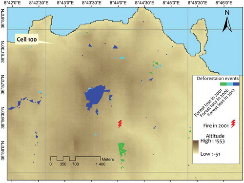
Raster files over the study area and period are loaded into the ArcGIS 10.4.1 (ESRI, Redlands, USA) and merged into a single mosaic. Each pixel in the resulting mosaic is assigned a value of 0, representing no forest loss, or a value from 1 to 14, representing loss detected primarily in the year 2001–2014, respectively. Figure 1 shows the map for the forest loss in the north regions of Tunisia for the period of study.

Figure 1. Map showing the forest loss in the northern Tunisia for the period 2000–2014.

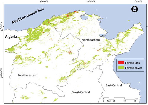
A validation exercise was also undertaken to ensure accurate data. Firstly, the forest-cover loss raster file was transformed into binary data (0, loss pixels; 1, no loss pixels). Next, a stratified random sampling scheme was performed. A visual interpretation was done based on validation sample points derived from higher-resolution imagery available on Google Earth. Respecting the number of checkpoints required to undertake a proper classification accuracy assessment, Congalton (2001) recommended a minimum number from 75 to 100 samples for each land-cover type when the scene is especially large. Congalton (2001) also suggested increasing the sampling on the loss class for generating a representative error matrix of the entire image classified. In our study, a total of 350 validation points (distributed as 200 and 150 for loss/no loss classes, respectively) for each year were used to carry out the accuracy assessment. Subsequently, the error matrix and its associated metrics of accuracy (i.e., overall-accuracy, producer’s and user’s accuracies) were computed.

Forest Fire Data

Fire data were sourced from the Fires Information for Resource Management (FIRMs) web interface (FIRMS 2015). FIRMs data are available for each overpass of the Moderate Resolution Imaging Spectroradiometer (MODIS) and lists the location of identified fires along. The hotspot detection is based on the algorithm by Giglio et al. (2010), which locates one or more fires (≥227°C) within a 1 km² pixel and assigns a confidence level based on the intensity of burning within each fire pixel (ranges from 0% to 100%). In some applications, errors of false alarms are particularly undesirable, and fires with a low confidence level (<30%) are not included (Giglio et al. 2010). Conversely, all datasets from 2001 to 2014 were retrieved in our study to ensure that no fires are missed.

Factors Data

Deforestation Factors

In addition to forest fires, anthropogenic interference and climate conditions are also major contributing factors to deforestation in Tunisia (Smirnakou, Ouzounis, and Radoglou 2017). The anthropogenic impact is due to the land-use change and wood harvesting activities, which have been increased significantly since 2011 (Chriha and Sghari 2013). We therefore considered four variables for each polygon of deforested area to describe the human pressure: (1) distance to major roads, (2) distance to minor roads, (3) distance to cities, and (4) distance to settlements. Concerning the climate conditions impact, the Mediterranean forests are very vulnerable to the deforestation because of the prolonged summer drought and the irregular rainfall (Larcher 2000). Mean annual rainfall and temperature data were then downloaded from Weather Underground site (http://www.weatherunderground.com) to reflect these climatic drivers. Other variables that influence the human accessibility to forest stands were included: distance to Algerian border, distance to sea, slope and altitude (Kalboussi and Achour 2018). All distance variables were derived from the agricultural maps from the DGF (2010) by using the Euclidean distance tool in ArcMap. Elevation data were derived from the 1-arc second DEM retrieved from the United States Geological Survey (USGS) website (http://www.earthexplorer. usgs.gov). Average slope and altitude were then computed for each polygon of deforestation using the Geoprocessing tool in ArcMap.

Forest Fire Factors

We used a variety of datasets for quantifying the causative factors of fire events. For each fire location, eight different input parameters were selected according to previous. The topographic factors affect the start and spread of fire (Castro and Chuvieco 1998; Chuvieco and Salas 1996) because they determine the airflow. Then, elevation, aspect and slope layers were produced using the DEM. The vegetation type is also one decisive factor. The fire moves faster through the easily flammable species such as Aleppo pine (Pinus halepensis) and often dies down when surrounded by less flammable species such as kermes oak (Quercus coccifera) (Chriha and Sghari 2013). Vegetation data were obtained from the national forest inventory map (DGF, Direction Générale des Forêts 2010). Anthropogenic-influenced localities are also areas of high fire risk because of the ignition source. Then, the distance from settlements and the distance from roads are regarded in our analysis. These two parameters were determined from the agricultural maps (DGF, Direction Générale des Forêts 2010). The date of fire ignition was also underlined to discern if it was a peak fire month or not. Generally, the most active fire months in Tunisia are August and July.

Spatio-temporal Data Mining Approach

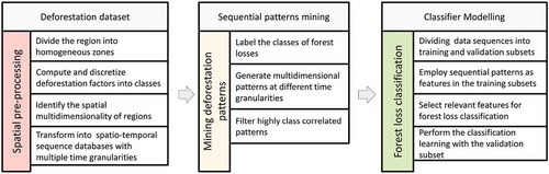
Figure 2 shows the three main stages of the proposed spatio-temporal data mining approach. First, the deforestation dataset is transformed into spatio-temporal sequence databases with considering two types of multidimensionality: (i) the spatial multidimensionality of regions (ii) and the multiple granularities of time. Then, these databases are mined to extract frequent deforestation patterns able to be used as distinctive features for classification. Finally, the most distinctive patterns are identified using feature selection to build the classifier. The following sub-sections describe the three phases in more detail.

Figure 2. Stages of the spatio-temporal data mining approach for forest loss estimation.

Spatial Pre-processing

The aim of t this phase is to transform the data into sequences according to a given spatial correlation structure or pattern. One of the goals of this study is to aggregate the close relationship between deforestation and forest fires, since they are considered as one of the major indicators in explaining the forest losses worldwide (Balch 2014). For this purpose, the spatial decomposition performed to divide the space into homogeneous zones should be determined according to the correlation between forest losses and fires. We superimposed a grid of 4 km x 4 km cells (Fishnet) over the deforested areas in Tunisia from 2000 to 2014 (Figure 3).

Figure 3. The grid cells over deforested areas in Tunisia for the period 2001–2014, and the close-up view of the locations of forest losses and fires in the selected grid cells (red box).

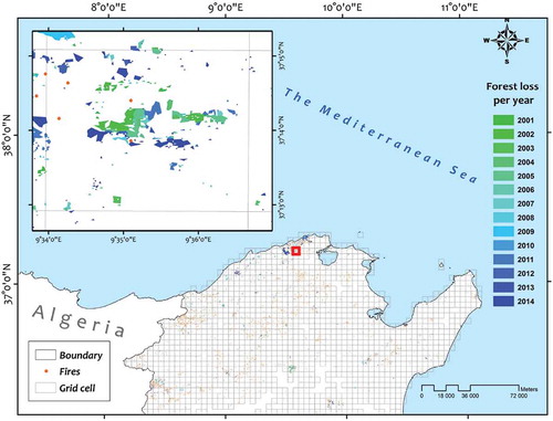
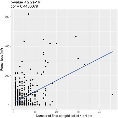
This higher-resolution grid is a way to reduce the inclusion of agricultural fires in the analysis (Portillo-Quintero, Sanchez-Azofeifa, and Do Espirito-Santo 2013). This scale is also proportional to the forest management unit whose mean area not exceeding 20 km². Significant correlation (r = 0.45; p < .01) between the total number of fires occurring in each grid cell and the average annual deforestation were observed (Figure 4). Therefore, there was a significant relationship between fires and the density of deforest areas. It equally confirms the reliability of the scale (16 km2). In total, 1743 grid cells over Tunisia were generated using Hawth’s Tool extension in ArcGIS 10.4.1.

Figure 4. Scatterplot of the total number of fires occurring in each grid cell and the forest loss for the 2001–2014 period. The Pearson coefficient of correlation is given as 0.489.

Thanks to this spatial division method, we are able to group deforestation events, including those of fires, within areas and thus to aggregate data concerning deforestation factors. These factors are determined by calculating the average values of their parameters for all deforestation polygons found per year within a grid cell. In contrast, since there are few cases where more than one fire occurrence is found per year within a grid cell, the corresponding factor parameters are directly assigned. As a result, the deforestation data set consists of 10 features and 6,284 rows, while the fire data set consists of 6 features and 2,611 rows. For instance, Table 1 illustrates the spatiotemporal factors for all deforestation and fire events occurring in the cell 100 during the period of study. While no fires occurred in 2006 and 2012, the deforestation events of 2001 have been accompanied by one fire occurrence. Figure 5 illustrates the occurrence of these events.

Table 1. Deforestation and fire events within the cell 100 and their spatiotemporal factors.

Events	Factors	2001	2006	2012
Deforestation	Altitude (Average in m)	107	175.5	243.222
	Slope (Average in %)	21.982	12.398	20.552
	Distance to cities (Average in m)	3492.569	1538.970	1840.510
	Distance to Algerian border (Average in m)	7052.660	7022.335	7173.881
	Distance to major road (Average in m)	1685.989	141.421	669.931
	Distance to minor road (Average in m)	113.514	75	739.112
	Distance to settlements (Average in m)	2827.396	2657.535	2490.558
	Distance to cities (Average in m)	2827.396	2657.535	2490.559
	Distance to sea (Average in m)	2751.820	2751.820	2751.820
	Average rainfall (in mm per month)	17.201	26.978	17.070
	Average temperature (in C° per month)	20.905	20.659	20.95
Forest fire	Altitude (in m)	763
	Slope (in %)	40.11
	Distance to Algerian border (in m)	2717.08
	Distance to road (in m)	862.4
	Distance to settlements (in m)	10100.5
	Vegetation type	scrab

Figure 5. Forest fires and deforestation events covered by cell 100.

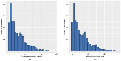
The next step is to code these spatiotemporal data into a sequence database in order to extract sequential patterns able to be used for the classification of forest losses. At the outset, continuous attributes should be discretized. Frequency histograms are studied for each attribute factor to determine the most appropriate discretization method. In our case, the components are well separated in frequency, and the observations are sufficient. Accordingly, the frequency distribution yields a good estimation of classes. Figure 6a,b show examples of frequency distribution for factors distance from nearest settlement to fire and the average altitude for deforested areas, respectively. Therefore, the equal frequency binning is the most appropriate in our case. This discretization method ensures that bins contain approximately the same number of components. So we obtain balanced classes for each attribute. Tables 2 and 3 describe parameters and their cut points for the deforestation factors and fire factors, respectively. Next, the data belonging to the same cell are grouped into sets and sorted by the time order. We thus get one chronological sequence of deforestation events for each grid cell. In this way, basic sequence mining algorithms can be applied to this database for extracting frequent sequences able to be represented as spatiotemporal patterns. Each grid cell is thus represented by the sequence of factors driving the deforestation and fire events that occurred into it. It is called the data sequence of the cell (Seq). For instance, the Seq for the cell 100(cell₁₀₀) is as follows: Seq₁₀₀ = <(fire_alt_165+, fire_slop_24.88+, fire_road_520.22+, fire_border_0-10288.29, fire_sett_5923.68+, fire_veg_scrab, alt_69-202, slope_13.96–22.90, sea_0-8602.8, border_0-30652.5, c_road_1555-3309.5, nc_road_87.27–177.31, cities_0-5486, sett_1802.8–2931.2, rain_0-19,temp_20.8–20.95)(alt_69-202, slope_7.3–13.95, sea_0-8602, border_0-30652.5, c_road_0-741.78, nc_road_0-87.27, cities_0-5486, sett_1802.8–2931.2, rain_25.5+, temp_20.8–20.95)(alt_203-413, slope_13.96–22.90, sea_0-8602.8, border_0-30652.5, c_road_0-741.78, nc_road_375+, cities_0-5486, sett_1802.8–2931.2, rain_0-19, temp_20.8–20.95)>. The matching Seq is composed of 3 time stamps (in 2001, 2006 and 2012) and the set of associated factors. Since the deforestation events in 2001 were accompanied by a fire occurrence, sets of factors influencing this fire and those influencing the deforestation events are presented together in the first stamp.

Table 2. Discretization of deforestation factor values.

Deforestation factors	Attributes	Cut points
Altitude (Average in m)	alt	68.5; 203; 413
Slope (Average in %)	slope	7.307; 13.96; 22.9
Distance to cities (Average in m)	sea	8602.8; 23293.3; 55680.5
Distance to Algerian border (Average in m)	border	30652.5; 7737.617; 132095
Distance to major road (Average in m)	c_road	741.78; 1555.03; 3309.46
Distance to minor road (Average in m)	nc_road	87.268; 177.308; 375
Distance to settlements (Average in m)	sett	1802.8; 2931.234; 4955.44
Distance to cities (Average in m)	cities	5486.003; 10381.156; 16269.299
Distance to sea (Average in m)	sea	8602.8; 23293.7; 55680.5
Average rainfall (in mm per month)	rain	19.079; 21.594; 25,413
Average temperature (in C° per month)	temp	20.571; 20.813; 20.95

Table 3. Attributes of fire factors and their domains and cut points.

Fire factors	Attributes	Domains and cut points
Altitude (in m)	fire_alt	165; 342; 602
Slope (in %)	fire_slop	7.70; 14.74; 24.88
Distance to road (in m)	fire_road	100; 250; 520.22
Distance to Algerian border (in m)	fire_border	10288.3; 53155.3; 93694.5
Distance to settlements (in m)	fire_sett	2256.1; 3701.35; 5923.68
Fire months	fire_month	May, June; July; August; September, October

Figure 6. (a) Frequency histogram for factor distance from nearest settlement to fire. (b) Frequency histogram for factor of average altitude for deforested areas.

Once the generated Seqs are ready for all grid cells, they can be used as input for a classical frequent sequential pattern mining algorithm. Generated patterns from this algorithm can be then used as features for a classifier of forest losses. To increase its accuracy, we tend to provide more informative deforestation patterns and compare their outcomes with those of conventional sequential patterns. A region is an area that has certain unifying characteristics such as climate, type of soil, substrate and relief. These characteristics that do not change over time strongly influence forest health and vegetation pattern. To examine how these further factors, that are more static, interact with deforestation profile, we should discriminate the grid cells using some of them. To do so, we adopt the concept of multidimensional sequential patterns proposed by Pinto et al. (2001) to extend sequences with these characteristics. For instance, the multidimensional sequence (MD-Seq) of cell₁₀₀ is exemplified in the following form: MD-Seq₁₀₀ = [region_Northeastern, clim_sub-humid, road_density_0.167–0.237, stream_density_374.709+, urban_1.63+, mean_alt_60.484–186.801, mean_slop_7.105–10.914]Seq₁₀₀, or MD-Seq₁₀₀ = [M₁₀₀] Seq₁₀₀, with MD-Seq₁₀₀ indicates Seq₁₀₀ in its multidimensional form and M₁₀₀ = {region_Northeastern, clim_sub-humid, road_density_0.167–0.237, stream_density_374.709+, urban_1.63+, mean_alt_60.484–186.801, mean_slop_7.105–10.914} is the set of multi-dimensional information for cell₁₀₀. Table 4 illustrates the multidimensional attributes used for this study and their domains and the cut points used to discretize continuous values.

Table 4. Multidimensional parameters of grid cells and their domains and cut points.

Multidimensional parameters	Description	Attributes	Domains and cut points
Planning region	The governorate where the grid cell is situated	region	Northwestern; Northeastern; West-Central; East-Central; Southern
Climate	The climate dominating the grid cell	clim	Saharan; semi-arid; arid; sub-humid; humid
Road density (in 100 km per 1 km^2)	The density of roads within the grid cell	road_density	0.1666; 0.2372; 0.3190
Stream density (in m per 1 km^2)	Stream length per grid cell	stream_density	374.7088
Mean altitude (in m)	The mean altitude across the grid cell	mean_alt	60.4841; 186.8011; 406.1228
Mean slope (in %)	The mean slope computed to the grid cell	mean_slop	7.1053; 10.9137; 17.0184
Urban occupation (in %)	The percentage of urban area within a cell	urban	1.63

A second multidimensionality component we examine to discover more informative patterns is the multiple time granularity. Actually, deforestation patterns can be observed only up to certain time scales, and thus capturing their variability at multiple time granularities could be useful to detect more informative patterns. This simulation involves two steps: (i) partitioning each sequence into many sub-sequences with different levels of granularity, and (ii) mining them according to the time granularity in order to capture temporal dependencies between deforestation patterns and classes. As we discussed previously, in four years since the Tunisian Revolution, forest losses have significantly exceeded the habitual rate. For that reason, we segment the time-line of the data sequences into two non-overlapping windows. The first is concerned with the period of before the Revolution (2001–2010). The second covers the next transition years (2011–2014). Continuing with the same example, generated sub-sequences for cell₁₀₀ are as follows: MD₁-Seq₁₀₀ = [M₁₀₀] < (fire_alt_165+, fire_slop_24.88+, fire_road_520.22+, fire_border_0-10288.29, fire_sett_5923.68+, fire_veg_scrab, alt_69-202, slope_13.96–22.90, sea_0-8602.8, border_0-30652.5, c_road_1555-3309.5, nc_road_87.27–177.31, cities_0-5486, sett_1802.8–2931.2, rain_0-19, temp_20.8–20.95) (alt_69-202, slope_7.3–13.95, sea_0-8602, border_0-30652.5, c_road_0-741.78, nc_road_0-87.27, cities_0-5486, sett_1802.8–2931.2, rain_25.5+, temp_20.8–20.95) > and MD₂-Seq₁₀₀ = [M₁₀₀] < (alt_203-413, slope_13.96–22.90, sea_0-8602.8, border_0-30652.5, c_road_0-741.78, nc_road_375+, cities_0-5486, sett_1802.8–2931.2, rain_0-19, temp_20.8–20.95) >, with MD₁-Seq₁₀₀ is the sub-sequence of MD-Seq₁₀₀ for the period of 2001 to 2010 and MD₂-Seq₁₀₀ is for the period after the Revolution. The next step for mining these multidimensional sequential patterns at multiple time granularities is depicted in the following subsection.

Deforestation Pattern Mining

The aim of this phase is to generate sequential patterns that are operated as candidate features for the classification of forest losses. The procedure consists of three main steps: (1) assign the class label of forest losses to each sequence in the database, (2) mine per time granularity the frequent patterns for each class label, (3) and filter highly discriminative and class correlated patterns. Figure 7 shows inputs, outputs and parameters used at each step.

Figure 7. Steps for the deforestation pattern mining stage.

Step 1 Class Labeling of Forest Losses

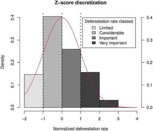
We computed the annual rate of forest losses for each grid cell, using “Tabulate Area” function in ArcGis 10.4.1, by dividing the sum of deforested areas by years of follow-up. The deforestation rate is shown in Figure 8a, denoting a positive skew, with the majority of the forest losses presenting a small rate. Thus, the logarithm function y = ln(x + 1) was applied to improve symmetry (Figure 8b). Since the log transformation yielded a nearly normal distribution (Menard 2002), the deforestation rate was discretized using the standardized normalization technique (z-score). We first compute the z-score of transformed variable for each sample as (x-μ)/σ, where μ is the mean and σ is the standard deviation. Then, we assign discretized values to samples according to their z-score using the following formula: “If |normalized deforestation rate| < −1, then it is limited; else if −1 ≤|normalized deforestation rate|<0, then it is considerable; else if 0≤|normalized deforestation rate| <1, then it is important; else it is very important” (Figure 9). Finally, before proceeding to the pattern mining phase, the dataset is partitioned into two subsets, one for training and one for validation.

Figure 8. The histogram for the deforestation rate (a) and respective logarithm transform (b).

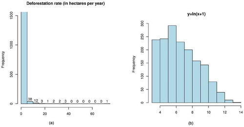
Figure 9. Class labeling of forest losses using the Z-score method.

Step 2 Mining Sequential Patterns

For each class in the training subset, frequent sequential patterns were extracted per time granularity. As indicated in the spatial pre-processing sub-section, we used a multi-dimensional sequence database as defined by Pinto et al. (2001). However, there is a problem when using the pattern mining algorithm by Pinto et al. (2001) that the redundancy in the results is considerable. For this reason, we choose to use the algorithm proposed by Songram et al. (2008) for mining frequent closed multidimensional sequential patterns. It allows performing a closed search of frequent patterns. This means that it only returns patterns that are not included in longer patterns, and then eliminates a great deal of redundancy without any information loss. Moreover, the algorithm by Songram and Boonjing (2008) is more efficient than the one of Pinto (2001) in terms of execution time and memory usage (Songram et al. 2008).

Step 3 Filtering Discriminative Patterns

The previous step usually obtains a large number of findings in spite of only mining-closed patterns. We would like to filter highly class correlated patterns and remove redundant patterns. To do so, we select for every time granularity level the set Disc-Seq of sequences that have a support above the required threshold minsup in one and only one class label partition. These patterns are distinctive for one class, i.e., occur frequently in that forest loss class, but at the same time they are infrequent in other classes. It should be noted that there are similar patterns that occur in sequences of different classes, but the time granularity of these patterns is different, which also makes them interesting patterns. For this reason, we apply the filter for each time granularity and not for all the patterns together. Figure 7 shows an illustrative simulation. For this instance, four patterns are eliminated by applying the filter: two patterns without time granularity reasoning and two others at the time granularity level 2.

Classifier Building

At this phase, we employ the set of discriminative sequential patterns (Disc-Seqs) as features, and we use the validation subset for building the sequence classifier. There are three steps necessary to do this: (i) transform the validation sequences into usable form for classification, (ii) identify the most discriminant subset of features using a feature-selection algorithm, and (iii) perform the classification learning using the selected features.

Step 1 Pre-processing of Classification Data

The first step in building the classifier is to pre-process the validation subset to prepare them for machine learning algorithms. For this purpose, we use Disc-Seqs to map validation sequences to binary feature vectors. Firstly, we check, for each sequence MD-Seq in the validation subset, if every feature in Disc-Seqs exits according to the time granularity level, using the following rule: If a feature Disc-Seq is in a sequence MD-Seq, then the corresponding feature has the value 1, otherwise the feature has the value 0. Assuming that we have n sequences in the validation subset and m features, this step will result in n vectors where each one contains m Boolean features.

Step 2 Feature Selection

A feature-selection algorithm is applied to the validation subset of input feature vectors, so that only the most discriminative features are used for the classifier construction. In doing so, this step will reduce the redundant features for a second time, and allow to predict the output class with accuracy comparable with that of classification using all features. Two feature-selection methods are commonly used; filter and wrapper methods (Saeys, Inza, and Pedro 2007). Wrapper methods select features with high prediction performance estimated by the learning algorithm that will be employed. Thus, they “wrap” the selection process around the learning algorithm. Whereas filter methods assess the relevance of features, independently of the learning algorithms, by ranking them according to certain scoring schemes such as information entropy and statistical dependence test. For this work, we employ the filter method, which is known to be computationally fast and independent of the choice of classifier. Moreover, it provides more generic set of features that is not biased or tuned by the learning algorithm and; hence the tendency to over-fitting is reduced (Guyon and Elisseeff 2003).

Step 3 Classifier Learning

In this last step, the selected features are then able to be processed as input vectors in any learning classification algorithm. The validation subset is used again during the training and classification phases. It should be noted that our classifier provides flexibility not only when choosing the learning algorithm but also when choosing the feature selection and sequential pattern mining algorithms.

Results and Discussion

Data Analysis

The validation exercise was performed on an annual basis from 2001 to 2014 through contingency matrix analysis. Figure 10 summarizes the resulting statistics (overall accuracy, user’s and producer’s accuracies). The validation points were retrieved from a visual interpretation of high-resolution Google earth images.

Figure 10. Accuracy measures of the data validation exercise.

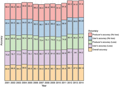
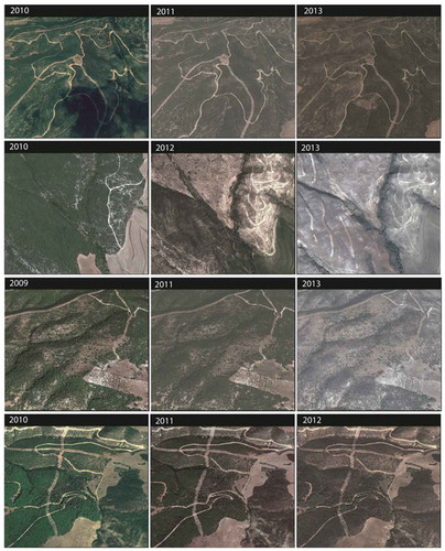
Figure 11 is a set of Google Earth images, illustrating some of the changes in the forest area. As displayed in Figure 10, the overall accuracy (OA) varies from 81.8% in 2001 to 88.1% in 2014, with an average of 86%. By and large, these results are consistent since the OA was relatively higher than the value of 85% established by Foody (2002) as acceptable. By contrast, on an annual basis, the OA values have failed to exceed this threshold for the years 2001, 2003 2007, 2008, and 2010. For all years from 2001 to 2014, producer’s and user’s for the “No loss” class are higher than for the “loss” class. In total, the “No loss” class has a user’s accuracy of 86%, while it is much lower for the “loss” class with an average of 81%. Regarding the producer’s accuracy, the “no loss” class also attained higher values than the “loss,” with an average of 90% and 80%, respectively.

Figure 11. Examples of validation points retrieved from Google earth imagery.

After confirming the accuracy of collected data, 44,169 polygons for “loss” class were extracted and grouped by year and grid cell. As described before, the deforestation factors for these polygons and those of fires were calculated and saved into tabular form, consisting of 6,255 rows (according to the number of deforestation events). Finally, the data after discretizing them were stored in three multidimensional sequence databases (MD-SD), each one covering one of the three different times granularity levels following the format described in Section 2.2.1. Hence, according to the number of grid cells, each MD-SD contains a total of 1784 sequences. For this database, 40% and 60% of data are used for training and validation, respectively. That is, sequences in their different granularity levels used for training are not used to build and to test the classifier. In order to generate stable results, we have to take into account of the spatial variability and the distribution of the classes. Therefore, sequences from the same forest loss class were distributed between planning regions according to the setup specified in Table 5. In this way, all regions in Tunisia are adequately covered by the training and the testing sets, and we mitigate the over-fitting problem.

Table 5. Repartition of training sets by planning regions and forest loss classes.

Planning region	Limited	Considerable	Important	Very important
Northwestern	49	90	54	36
Northeastern	70	117	57	44
West-Central	16	33	21	12
East-Central	8	16	12	10
Southern	10	14	24	16

Mining Deforestation Patterns

The application of Songram algorithm to the training subset resulted in high frequent closed multidimensional sequential patterns by using a minimum frequency threshold of minsup = .15. The mining process was terminated at 324, 207, 338 and 345 patterns for classes, “Limited,” “Considerable,” “Important” and “Very important”, respectively. The total number per time granularity was 786, 81 and 347 for the periods 2000–2014, 2000–2010 and 2011–2014, respectively. Some of these patterns are presented per class and per time granularity in Table 6.

Table 6. Some multidimensional sequential patterns at different time granularities.

Time granularity	Classes	Multidimensional sequential patterns	Support
2000–2014	Limited	[mean_alt_406.123+]< (alt_467.7+; sea_55680.5+) >	0.26
	Considerable	< (temp_20.8–20.95) (temp_20.95+; rain_0-19.079) >	0.34
	Important	< (temp_0-20.57) (rain_0-19.08; temp_20.57–20.81) (temp_20.95+) >	0.51
	Very important	< (temp_0-20.57) (rain_0-19.08; temp_20.57–20.81) (temp_20.95+) >	0.31
2000–2010	Limited	[climate_semi-arid]< (fire_month_August; temp_20.95+) >	0.15
	Considerable	[mean_alt_406.123+]< (temp_20.95+) >	0.27
	Important	< (slope_22.9+;cities_16269.3+) (slope_22.9+) >	0.22
	Very important	[stream_density_0-374.71] < (temp_0-20.57) (rain_0-19.08) (temp_20.95+) >	0.47
2011–2014	Limited	[urban_0-1.63] <(sett_0-2256.1; c_road_0-741.78; nc_road_0-87.268)>	0.23
	Considerable	[climate_semi-aride]<(sett_0-2256.1)>	0.16
	Important	<(fire_road_515.39+; sea_0-8602.8) (sea_0-8602.8)>	0.25
	Very important	<(fire_month_July; nc_road_375+; border_0-30652.5)(border_0-30652.5)>	0.33

The support of the 8th pattern in Table 6 means that the sequence “[stream_density_0-374.71] <(temp_0-20.57) (rain_0-19.08) (temp_20.95+)>”appears for 47% of cells labeled with the class “Very important” for the period of 2000–2014, and can be interpreted as the increase of the temperature over time, marked with the lowest amount of rainfall, can be one of the significant factors causing the very important rate of deforestation between 2000 and 2014, specially in regions with minor stream density. Extracted patterns represent the evolution of a set of spatial factors and their combinatory effects on the rate of deforestation within the defined cell area. For samples, it could be concluded from the patterns 3 and 4 that the successive years of drought can cause very high rates of forest loss (as reflected by the continuous increase of temperature and the decrease of the annual rainfall amount). The support of patterns can manifest the importance of factors that may differ in impacts across different regions or times. For example, the supports of patterns <(fire_month_July; nc_road_375+; border_0-30652.5) (border_0-30652.5) > “ and “[climate_semi-arid] <(fire_month_August; temp_20.95+) >” (0.33 and 0.15, respectively) and their class labels (“Very important” and “Limited”, respectively) may expose that fires occurring far from roads and close to Algerian borders are more intensive than fires fueled by August’s drought. According to the time granularity, this pattern “<(fire_month_July; nc_road_375+; border_0-30652.5) (border_0-30652.5)>“, that is associated to the after-Revolution period, can reflect the increase of illegal activities, including deforestation and human-induced fires. This phenomenon is also confirmed by the 11th pattern <(fire_road_515.39+; sea_0-8602.8) (sea_0-8602.8)>that can point out the expanding human settlements in coastal forest region after the Revolution. As mentioned before, we generated closed multidimensional sequential patterns for different levels of time granularity to have more informative patterns. To evaluate their efficiency for building our classifier, we compared their outcomes with those of other standard sequential patterns. We used ClaSP algorithm (Gomariz et al. 2013) to mine closed sequential patterns without consideration of any spatial multidimensionality. The ClaSP is generally faster than other algorithms for closed sequential patterns such as CloSpan (Yan, Han, and Afshar 2003) and BIDE+ (Wang, Han, and Li 2007). Similarly, we applied this algorithm to sequence database with and without taking into account the time granularity to assess the influence of neglecting this information. All in all, it has three subsets of patterns to test, closed multidimensional sequential patterns with time granularity (1st subset), closed multidimensional sequential patterns without time granularity (2nd subset), and standard closed sequential patterns (3rd subset).

Next, in the post-processing step, we retained the highly class correlated patterns. As an example of this, the 3rd and the 4th from Table 6 were dropped given that two classes (“Important” and “Very important”) are characterized by a same pattern “< (temp_0-20.57) (rain_0-19.08; temp_20.57–20.81) (temp_20.95+) >”. This filter was performed per time granularity on the first subset as explained before. In total, 61, 45 and 37 patterns were retained from the first, the second and the third subsets, respectively.

Classifier Performance

For training and testing the classifier, we used the implementations provided by the Weka machine learning environment (Machine Learning Project 2017). For the feature-selection step, we investigated two algorithms Random Forests (RF) (Hastie, Tibshirani, and Friedman 2009) and Support Vector Machine (SVM) (Schölkopf and Smola 2002). The RF method returns a subset of features to be used for training the classifier, while the SVM method returns a ranked list of features. All selected features were retained using the RF method. However, by using SVM we consider the top l features when building the classifier. After pecking the relevant features, we applied the Random Forest classifier on the validation subset. We calculated 10-fold cross-validation classification accuracy for each class of forest losses. Four metrics were used in evaluating the classifier’s accuracy: precision, recall, F-measure, and operating characteristic curve (ROC).

The RF method returned 42, 47 and 51 features from the 1st, 2nd and 3rd subset, respectively. Thus, results of SVM method are evaluated for l = 40, 45 and 50 for the 1st subset, and for l = 45, 50 and 55 for the 2nd and 3rd subsets. Table 7 lists the results for the classifier when using the various top-l features. The results from the SVM method are highly similar within each of the three subsets. However, by an inter-comparison, the classification results using the closed multidimensional sequential patterns are clearly better. On the other hand, the results when using standard patterns (3rd subset) were significantly lower than others. A preliminary interpretation indicates the advantage of employing more informative patterns by integrating time granularity and spatial multidimensionality components. This finding can be also confirmed by looking at the number of selected features when using the RF method. The number of features increased when including time granularity and/or spatial multidimensionality components.

Table 7. The average ROC scores using different subsets and parameters of top-l features.

Patterns	1st subset			2nd subset			3rd subset
Top-l features	40	45	50	45	50	55	45	50	55
ROC	0.826	0.852	0.852	0.660	0.685	0.685	0.581	0.597	0.601

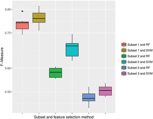
To compare the SVM feature-selection method to the RF one, we draw on the best results for each subset of patterns (0.852, 0.685 and 0.601 for the 1st, 2nd and 3rd subset, respectively). Table 8 sets out the results of this comparison, which also show the contributions made by patterns to the classification accuracy. Obviously, the RF method returns a result slightly less accurate than that obtained by SVM method for all subsets, with an F-measure of 0.832, 0.820 and 0.811 compared to 0.796, 0.772 and 0.785. However, the difference provided by the patterns is very significant, where the use of closed multidimensional sequential patterns at multiple time granularities allows more accurate results. The use of standard patterns provides low accuracy for both SVM and RF methods with an F-measure of 0.505 and 0.477, respectively. The reason behind the difference in these results is that patterns specified by more information about time granularity and spatial characterization are more discriminative for the level of forest loss. Conversely, standard patterns contain more redundant information, leading to a less reliable estimation. When considering the 10-fold cross-validation tests, a similar interpretation emerges, as displayed in Figure 12. In all tests, both SVM and RF methods perform better when using the 1st subset than when using the others, approving the superiority of proposed informative patterns for our classifier.

Table 8. Average recall, precision and F-measure using the different feature-selection methods and subsets.

Feature selection	SVM method			RF method
Metrics	Recall	Precision	F-measure	Recall	Precision	F-measure
1st subset	0.832	0.820	0.811	0.796	0.772	0.785
2nd subset	0.615	0.666	0.683	0.597	0.611	0.580
3rd subset	0.577	0.476	0.505	0.334	0.431	0.477

Figure 12. Boxplots of different F-measures of the 10-fold cross-validation tests over different methods (SVM and RF methods) and subsets (1st, 2nd and 3rd subsets).

Thus, as expected, these patterns reflected properly the high-influence of the Revolution. The accuracy improvement was predominantly because of the integration of patterns of before and after the Revolution. Actually, it is evident that any political instability will naturally lead to a serious ecological stress (Sangne et al. 2015). In Tunisia, because of the administration feebleness in the post-Revolution period, the forest ecosystem finds itself victim of large-scale depredations (Chakroun et al. 2012). For example, the illegal logging has increased hugely since 2011 and reached its highest ever reported level in 2013, when more than 110,160 illegally harvested trees were recorded against 7,530 in 2007. Another major factor underlined by tested patterns is the forest fires. The spatial decomposition was performed based on the correlation between fires and deforested areas, and also the driving factors of forest fires were suggested as ones of potential deforestation drivers. As remarked in Table 6, many fire factors were revealed in patterns, demonstrating that fires were significant contributing factors to the rising levels of forest loss. By Chriha and Sghari (2013), forest fires after the Revolution are deliberately triggered to allow the spontaneous grabbing of devastated land. In 2012, approximately 493 fires were recorded in Tunisia, 229 greater than those recorded in 2010 (San-Miguel-Ayanz et al. 2012).

Lastly, looking at the efficiency of the two feature-selection algorithms, the SVM method performs slightly better than RF method. However, as practice shows, selecting the right number of features is not an easy task when using SVM method. From this point of view, the RF method could be more convenient since it simply selects a well-defined subset of features.

Conclusion

This study demonstrates a novel spatio-temporal pattern-based sequence classification approach for forest loss estimation. This approach was performed with two datasets of high availability and high readiness, (i) time series of 15-year of satellite images and (ii) historical wildfire GIS data. Results demonstrate that more than 85% of the time the forest losses can be fittingly estimated. From this, it can be concluded that the pattern representation we propose is adapted to the Tunisian case study. Sequences were associated with multiple spatial dimensions and multiple time granularities to better consider the high spatial variability of regions and the Revolution impacts, respectively. Moreover, the proposed approach can be applied to other locations and even to other spatio-temporal problems, since it follows the same steps as the general data mining process. A limitation of this research is that sequential patterns have been used merely as classification features, even though they can be analyzed and evaluated using information visualization techniques. Thus, directions for future work include some of these techniques to visualize and analyze spatiotemporal patterns of deforestation threat.

Acknowledgments

We are very grateful for the cooperation and friendship with the staff of the Tunisian General Directorate of Forestry.

References

- Aggarwal, C. C. 2014. Applications of frequent pattern mining. In Aggarwal C., Han J. (eds.), Frequent Pattern Mining (pp. 443-467). Springer, Cham.
- Ahn, Y. S., S. R. Ryu, J. Lim, C. H. Lee, J. H. Shin, W. I. Choi, B. Lee, J. H. Jeong, K. W. An, and J. I. Seo. 2014. Effects of forest fires on forest ecosystems in eastern coastal areas of Korea and an overview of restoration projects. Landscape and Ecological Engineering 10 (1):229–37. doi:10.1007/s11355-013-0212-0.
- Akbari, M., F. Samadzadegan, and R. Weibel. 2015. A generic regional spatio-temporal co-occurrence pattern mining model: A case study for air pollution. Journal of Geographical Systems 17 (3):249–74. doi:10.1007/s10109-015-0216-4.
- Alatrista-Salas, H., J. Azé, S. Bringay, F. Cernesson, N. Selmaoui-Folcher, and M. Teisseire. 2015. A knowledge discovery process for spatiotemporal data: Application to river water quality monitoring. Ecological Informatics 26:127–39. doi:10.1016/j.ecoinf.2014.05.011.
- Balch, J. K. 2014. Atmospheric science: Drought and fire change sink to source. Nature 506 (7486):41. doi:10.1038/506041a.
- Campos, P., H. Daly-Hassen, J. L. Oviedo, P. Ovando, and A. Chebil. 2008. Accounting for single and aggregated forest incomes: Application to public cork oak forests in Jerez (Spain) and Iteimia (Tunisia). Ecological Economics 65 (1):76–86. doi:10.1016/j.ecolecon.2007.06.001.
- Castro, R., and E. Chuvieco. 1998. Modeling forest fire danger from geographic information systems. Geocarto International 13 (1):15–23. doi:10.1080/10106049809354624.
- Chakroun, H., F. Mouillot, M. Nouri, and Z. Nasr. 2012. Integrating MODIS images in a water budget model for dynamic functioning and drought simulation of a mediterranean forest in Tunisia. Hydrology and Earth System Sciences Discussions 5:6251–84. doi:10.5194/hessd-9-6251-2012.
- Chriha, S., and A. Sghari. 2013. Les Incendies de Forêt En Tunisie. Séquelles Irréversibles de La Révolution de 2011. Méditerranée. Revue Géographique Des Pays Méditerranéens/Journal of Mediterranean Geography 121:87–93.
- Chuvieco, E., and J. Salas. 1996. Mapping the Spatial Distribution of Forest Fire Danger Using GIS. International Journal of Geographical Information Science 10 (3):333–45.
- Congalton, R. G. 2001. Accuracy assessment and validation of remotely sensed and other spatial information. International Journal of Wildland Fire 10 (4):321–28. doi:10.1071/WF01031.
- Davies, D. K., S. Ilavajhala, M. M. Wong, and C. O. Justice. 2009. Fire information for resource management system: Archiving and distributing MODIS active fire data. IEEE Transactions on Geoscience and Remote Sensing 47 (1):72–79. doi:10.1109/TGRS.2008.2002076.
- DeFries, R. S., T. Rudel, M. Uriarte, and M. Hansen. 2010. Deforestation driven by urban population growth and agricultural trade in the twenty-first century. Nature Geoscience 3 (3):178. doi:10.1038/ngeo756.
- DGF, Direction Générale des Forêts. 2010. Résultats du deuxième inventaire forestier et pastoral national. Ministère de l’Agriculture de Tunisie, 180.
- Dong, G., and J. Pei. 2007. Sequence data mining, vol. 33. Springer Science & Business Media, Boston.
- FAO, I. 2016. WFP, The state of food insecurity in the World 2016. The multiple dimensions of food security. Rome: FAO.
- FIRMS, 2015. Fire information for resource management system FIRMS. accessed September, 2015. http://earthdata.nasa.gov/earth-observation-data/near-real-time/firms/
- Foody, G. M. 2002. Status of Land Cover Classification Accuracy Assessment. Remote Sensing of Environment 80 (1):185–201. doi:10.1016/S0034-4257(01)00295-4.
- Giglio, L., J. T. Randerson, G. R. Van der Werf, P. S. Kasibhatla, G. J. Collatz, D. C. Morton, and R. S. DeFries. 2010. Assessing variability and long-term trends in burned area by merging multiple satellite fire products. Biogeosciences 7 (3):1171–86. doi:10.5194/bg-7-1171-2010.
- Gomariz, A., M. Campos, R. Marin, and B. Goethals. 2013. ClaSP: An efficient algorithm for mining frequent closed sequences. Pacific-Asia Conference on Knowledge Discovery and Data Mining, 50–61. Springer.
- Guyon, I., and A. Elisseeff. 2003. An introduction to variable and feature selection. Journal of Machine Learning Research 3 (Mar):1157–82.
- Hansen, M. C., P. V. Potapov, R. Moore, M. Hancher, S. Turubanova, A. Tyukavina, D. Thau., Stehman S. V., Goetz S. J., Loveland T. R., Kommareddy A., Egorov A., Chini L., Justice C. O., Townshend J. R. G. High-resolution global maps of 21st-century forest cover change. Science. 342(6160):850–53. doi:10.1126/science.1244693.
- Hansen, M. C., and T. R. Loveland. 2012. A review of large area monitoring of land cover change using landsat data. Remote Sensing of Environment 122:66–74. doi:10.1016/j.rse.2011.08.024.
- Hastie, T., R. Tibshirani, and J. Friedman. 2009. The elements of statistical learning (Pp520-529). New York: Springer.
- Hietel, E., R. Waldhardt, and A. Otte. 2004. Analysing land-cover changes in relation to environmental variables in Hesse, Germany. Landscape Ecology 19 (5):473–89. doi:10.1023/B:LAND.0000036138.82213.80.
- Kalboussi, M., and H. Achour. 2018. Modelling the spatial distribution of snake species in Northwestern Tunisia using maximum entropy (Maxent) and Geographic Information System (GIS). Journal of Forestry Research 29 (1):233–45. doi:10.1007/s11676-017-0436-1.
- Kuzera, K., J. Rogan, and J. Ronald Eastman. 2005. Monitoring vegetation regeneration and deforestation using change vector analysis: Mt. St. Helens study area. ASPRS Annual Conference, Baltimore, MD.
- Larcher, W. 2000. Temperature stress and survival ability of mediterranean sclerophyllous plants. Plant Biosystems 134 (3):279–95. doi:10.1080/11263500012331350455.
- Lui, G. V., and D. A. Coomes. 2015. A comparison of novel optical remote sensing-based technologies for forest-cover/change monitoring. Remote Sensing 7 (3):2781–807. doi:10.3390/rs70302781.
- Machine Learning Project, 2017. Weka—Waikato environment for learning analysis. Accessed July 12, 2017. http://www.cs.waikato.ac.nz/ml/index.html
- Menard, S. 2002. Applied logistic regression analysis No. 106. Sage.
- Peduzzi, P., J. Concato, E. Kemper, T. R. Holford, and A. R. Feinstein. 1996. A simulation study of the number of events per variable in logistic regression analysis. Journal of Clinical Epidemiology 49 (12):1373–79. doi:10.1016/S0895-4356(96)00236-3.
- Pinto, H., J. Han, J. Pei, K. Wang, Q. Chen, and U. Dayal. 2001. Multi-dimensional sequential pattern mining. Proceedings of the Tenth International Conference on Information and Knowledge Management, 81–88, ACM, Atlanta, GA, United States.
- Portillo-Quintero, C., A. Sanchez-Azofeifa, and M. M. Do Espirito-Santo. 2013. Monitoring deforestation with MODIS active fires in neotropical dry forests: An analysis of local-scale assessments in Mexico, Brazil and Bolivia. Journal of Arid Environments 97:150–59. doi:10.1016/j.jaridenv.2013.06.002.
- Saeys, Y., I. Inza, and L. Pedro. 2007. A review of feature selection techniques in bioinformatics. Bioinformatics 23 (19):2507–17. doi:10.1093/bioinformatics/btm344.
- Sangne, C., Barima, Y., Bamba, I., & N’Doumé, C-T.. (2015). Dynamique forestière post-conflits armés de la Forêt classée du Haut-Sassandra (Côte d’Ivoire). [VertigO] La revue électronique en sciences de l’environnement, 15(3). doi:10.4000/vertigo
- San-Miguel-Ayanz, J., E. Schulte, G. Schmuck, A. Camia, P. Strobl, G. Liberta, C. Giovando, R. Boca, F. Sedano, P. Kempeneers, D. McInerney, C. Withmore, S. S. de Oliveira, M. Rodrigues, T. Durrant, P. Corti, F. Oehler, L. Vilar and G. Amatulli 2012. Comprehensive monitoring of wildfires in Europe: The European Forest Fire Information System (EFFIS). In Approaches to Managing Disaster-Assessing Hazards, Emergencies and Disaster Impacts. InTech. Available from: https://www.intechopen.com/books/approaches-to-managing-disaster-assessing-hazards-emergencies-and-disaster-impacts/comprehensive-monitoring-of-wildfires-in-europe-the-european-forest-fire-information-system-effis-
- Schölkopf, B., and A. J. Smola. 2002. Learning with Kernels: Support vector machines, regularization, optimization, and beyond. Cambridge, MA: MIT Press.
- Smirnakou, S., T. Ouzounis, and K. M. Radoglou. 2017. Continuous spectrum LEDs promote seedling quality traits and performance of quercus ithaburensis Var. Macrolepis. Frontiers in Plant Science 8:188.
- Songram, P., and V. Boonjing. 2008. Closed multidimensional sequential pattern mining. International Journal of Knowledge Management Studies 2 (4):460–79. doi:10.1504/IJKMS.2008.019752.
- Toujani, A., H. Achour, and F. Sami. 2018. Estimating forest fire losses using stochastic approach: case study of the Kroumiria Mountains (Northwestern Tunisia). Applied Artificial Intelligence 32(9-10), 882-906. doi:10.1080/08839514.2018.1514808.
- Traore, B. B., B. Kamsu-Foguem, and F. Tangara. 2017. Data mining techniques on satellite images for discovery of risk areas. Expert Systems with Applications 72:443–56. doi:10.1016/j.eswa.2016.10.010.
- Turco, M., M.-C. Llasat, J. von Hardenberg, and A. Provenzale. 2014. Climate change impacts on wildfires in a mediterranean environment. Climatic Change 125 (3–4):369–80. doi:10.1007/s10584-014-1183-3.
- Wang, J., J. Han, and L. Chun. 2007. Frequent closed sequence mining without candidate maintenance. IEEE Transactions on Knowledge and Data Engineering 19 (8):1042–56. doi:10.1109/TKDE.2007.1043.
- Yan, X., J. Han, and R. Afshar. 2003. CloSpan: Mining: Closed sequential patterns in large datasets. Proceedings of the 2003 SIAM International Conference on Data Mining, 166–77. SIAM, San Francisco, Calif, USA.
- Yusof, N., and R. Zurita-Milla. 2017. Mapping frequent spatio-temporal wind profile patterns using multi-dimensional sequential pattern mining. International Journal of Digital Earth 10 (3):238–56. doi:10.1080/17538947.2016.1217943.