Evolino Recurrent Neural Network Ensemble for Speculation in Exchange Market in Time of Anomalies

ABSTRACT

Sharp falls or explosive growths in exchange markets, whether expected or not, generates new challenges for investors who want to protect their investments or achieve an optimum benefit during and after the turmoil. An anomaly of the exchange market, instigated by the Swiss National Bank, occurred when the Swiss Franc decoupled from the euro unexpectedly. The United Kingdom (UK) vote to withdraw from the European Union (Brexit), in contrast, was feared but expected. A comparison of the consequences of the anomalies gives us an unprecedented opportunity to investigate prediction capabilities of the EVOLINO Recurrent Neural Network Ensemble (ERNN) model following an anomaly. By introducing this new information to the ERNN model and analyzing its response, we increase investor resources during large exchange rate fluctuations; this will provide them with additional information that will help them construct different portfolios. Reaction to the anomaly was visible only after the anomaly occurred, this is when the model began to acquire data influenced by the extreme change. Comparing different strategies which are related or unrelated to the anomaly and orthogonal or not orthogonal for conservative, moderate, or aggressive trading shows that in order to profit from the anomaly, speculation depends on prediction-accuracy and on the sets of exchange-rate associated with the anomaly.

Introduction

A sudden change in the financial market that conflicts with the effective market hypothesis and other patterns of consistent markets is called a financial market anomaly. A currency market anomaly is often a sharp fall in the exchange rate or sometimes – its explosive growth. Investors are interested in anomalies for two reasons: to save an investment or to benefit from the sharp fluctuations in exchange rates. Therefore, it is important to recognize anomalies in chaotic currency fluctuations and to prepare for any possible surprises.

Anomalies in the finance market can be expected or unexpected. Schwert (2003) investigated different effects of finance market anomalies: size, value, weekend, day-of-week, dividend-yield, and small-firm turn-of-the-year effects. Lamont and Thaler (2003) investigated the effects of low price in a financial market. Avramov and Chordia (2006) investigated asset pricing models in order to explain the size, value, and momentum anomalies. Stock market anomalies were later investigated in more detail. The most significant anomaly in economics is the “quality anomaly”; this occurs when stocks with high profitability ratios tend to outperform on a risk-adjusted basis (Novy-Marx 2013).

Investor behavior is an important variable in trading. Developing trading strategies and adhering to them, despite hope and fear, is often shaped by investor opinions about possible finance market changes. These predictions form the basis of investor expectations and their subsequent decisions. Ter Ellen, Verschoor, and Zwinkels (2013) tested three different strategies on the disaggregated expectations primarily, momentum trading, Private Placement Programs (PPP) trading and interest rate trading strategies. The study by Stambaugh, Yu, and Yuan (2012) explores the role of investor outlook for a broad set of anomalies in cross-sectional stock returns. They investigated three statements: the first, that the anomalies should be stronger following periods of optimistic investor outlook; the second, that the short-leg of each long-short anomaly strategy should have lower returns (greater profits) following optimistic outlooks than following negative outlooks, and finally, that sentiment exhibits no relation to returns on the long-leg of the strategies.

Finance market anomalies are closely related to changes in the economy. Kontonikas and Kostakis (2013) investigated the impact of United States monetary politics on stock market anomalies. Authors show that value, small capitalization and past loser stocks are more exposed to monetary policy shocks in comparison to growth, big capitalization and past winner stocks. The dynamic nature of stock prices are used like leading indicators in economic forecasting. Cella, Ellul, and Giannetti (2013) investigated a quantitative link between some market anomalies and investor behavioral biases. Research into endogenous growth examines the positive correlations between: stock returns and aggregate economic activity; stock returns and investment (Subrahmanyam and Titman 2013). Maghrebi, Holmes, and Oya (2014) investigated the short-term dynamics of volatility expectations during periods of financial instability. Shu and Chang (2015) investigated models that can adequately interpret prominent financial market anomalies, such as: high volatility; bubble and crash formation; the relationship between investor outlook and asset prices; the relationship between investor outlook and expected returns.

Portfolio construction is also an effective tool for trading in the stock market as it protects investments against unexpected changes in stock, exchange rate, or capital market. Israel and Moskowitz (2013) investigated different portfolios with different impact predictions of market anomalies. Chu, Hirshleifer, and Ma (2015) find that anomalies become substantially weaker on portfolios constructed with pilot stocks during the pilot period. This effect comes about from short periods of trading by anomaly portfolios. Bouchaud et al. (2016) proposed and tested a model that predicts that the quality (or “profitability”) anomaly arises if market participants update expectations of the future profits too slowly or if the level of profits can be predicted by persistent publicly observable signals. Novy-Marx and Velikov (2016) analyzed 23 of the best known, and strongest performing, anomaly strategies. The authors also quantify how much new capital could be devoted to trading each strategy before marginal traders and whether or not they would find the strategies profitable. Marginal traders are defined as those who trade the latest. The January effect and short-term autocorrelations of market returns were investigated by Jones and Pomorski (2016). The accounting for decay has a substantial impact on portfolio choice and allows anomalous returns to shrink over time. Predictive return models may be an important component of active investment strategies once those models allow for the possibility of decay.

Exchange markets anomalies are related to market inefficiency. Results of Li and Miller (2015) imply that the existence of forex market inefficiency is consistent with many puzzling facts about exchange rates. Market rationality is the dominant paradigm in order to organize and rule the markets. Yalcin (2016) investigated the possible reasons of observed market anomalies and whether they are the powerful sign for inefficiency of the market. Impact of anomalies of finance market to economic growth, solving financial fraud detection problems, an attempt to understand the irrationality of financial markets require the innovative tools for predicting and pattern recognition. Ahmed, Mahmood, and Islam (2016) present an in-depth survey of various clustering based anomaly detection technique and compares them from different perspectives.

Accurate prediction and financial anomaly identification using artificial intelligence tools are the important tasks for investors and speculators. Namazi, Shokrolahi, and Maharluie (2016) investigated the possibility of identification and ranking of significant factors that affect the free cash flow risks through artificial neural networks.

Unexpected events, anomalies are found not only in the financial markets; they are also found in: volatile climate changes like temperature, rainfall, extreme flooding, and spring snow; and catastrophes like earthquakes, tsunami, and many others. Scientists’ experience in predicting and recognizing anomalies has great value. Malhotra et al. (2015) use stacked Long Sort Time Memory (LSTM) networks for anomaly/fault detection in time series. A network is trained on non-anomalous data and used as a predictor over a number of time steps. Acharya et al. (2014) used the concept and the implementation strategy of extreme learning machine (ELM) and developed multi-model ensemble (MME) by implementing ELM approach to predict rainfall. The results of the paper depicted that the MME can efficiently predict extremes in rainfall. Zafari et al. (2014), Gupta, Kumar, and Kumar (2016) investigated the differential evolutionary and genetic algorithms used in finance market prediction. Prediction models, based on an ensemble of evolutionary neural networks, developed by physical scientists provide additional resources for financial analysts. In fact, the main component of Evolino is LSTM memory cell.

The aim of the paper is to investigate the anomalies of exchange market created by the unexpected Swiss National Bank (SNB) intervention and the expected the United Kingdom (UK) vote to withdraw from the European Union (EU) or Brexit. Our research investigated how the EVOLINO Recurrent Neural Network Ensemble (ERNN) model forecast reactions to anomalies. The next task was to examine the investors’ ability to save investments or make profit from large exchange rate fluctuations by constructing different portfolios.

Examples of Exchange Market Anomalies

The reasons for anomalies in exchange market can be very different: from natural disasters, wars, geopolitical events, banking interventions, and others. We observed some of them in a period of 5 years. Unfortunately, anomalies come on suddenly and so it is difficult to properly prepare for its investigation.

On 11 Mar 2011, Japan was shaken by a 9.0 magnitude earthquake that was followed by a tsunami. The tsunami caused nuclear accidents in the Fukushima Daiichi Nuclear Power Plant complex. Figure 1 shows reaction of exchange market to this natural disaster. The anomaly is labeled with a dash ellipse.

Figure 1. The reaction of EUR/JPY and USD/JPY to tsunami in Japan on 11 Mar 2011.

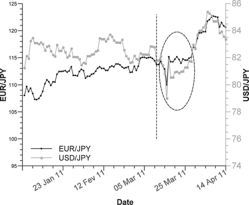
At the moment of disaster (vertical dash line), exchange rates did not react strongly: EUR/JPY maximal-minimal day values fell 2.082 points, open-close – 0.703, USD/JPY fell 1.642 and 1, respectively. The Bank of Japan offered 15 trillion (US 183 billion) to the banking system on 14 March in an effort to normalize market conditions. Problems with three reactors in the Fukushima Daiichi Nuclear Power Plant complex caused even greater market reactions: EUR/JPY daily max-min fell by 6,653 on 16 March, open-close – 2.915, on 17 March the max-min fluctuated 5.809 points, open-close growth was 5.188. USD/JPY daily max-min fell down 4,466 at 16 March, open-close 1.842, at 17 March max-min fluctuated 3.584 points, open-close growth 2.824. The Bank of Japan managed to stabilize the market and the currency market fluctuations and was normal by the end of March. Natural disasters and their effects on the country’s economy are hardly predictable. Investors, in this case, did not have big losses because the exchange rate quickly recovered or a “stop loss” was used.

On 15 January 2015, the Swiss National Bank (SNB) suddenly announced that it would no longer hold the Swiss franc at a fixed exchange rate with the euro. Investors like the Swiss franc as it is a safe asset with low risk. The Swiss government runs a balanced budget with low inflation in the country. In addition, large foreign-exchange reserves and other reasons make the Swiss franc stable and strong. So this banking intervention generated big losses for investors and a number of hedge funds across the world. Figure 2 displays the reaction of EUR/CHF and USD/CHF to the SNB action.

Figure 2. The reaction of USD/CHF and EUR/CHF to banking intervention 15 Jan2015.

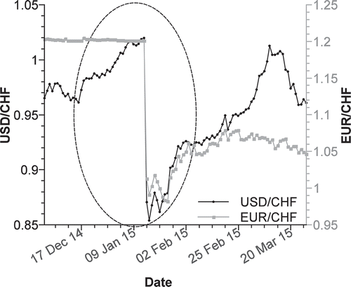
At the moment of banking intervention, on 15 of January 2015, the exchange market reacted very strongly: EUR/CHF fell 0.18805 points (max-min 0.23029), USD/CHF – 0.14917 points (max-min 0.18729). This was followed by a small rise, a fall again, and finally the exchange rates began to slowly stabilize. USD/CHF rebounded only in the middle of March, and the EUR/CHF remained approximately 0.13–0.14 points below the value at the time of the banking intervention.

Prediction of anomalies based on banking interventions depends on accurate and timely information. Informed investors who outsource can see a big benefit. Uninformed investors can be helped by luck or using “stop loss.” Losses can be reduced by diversifying risk via an orthogonal portfolio. Kvietkauskienė and Maknickienė (2015) compared losses at the moment of described anomaly using orthogonal and not orthogonal portfolios.

The third anomaly observed in the foreign exchange market is a political. The British exit from the European Union, or Brexit is an example of this. On 23 June 2016, British citizens voted for the UK exit from the EU. It was possible to expect and anticipate that the market would react, whatever the outcome of the vote. Figure 3 shows the reaction of EUR/GBP and GBP/USD due to voting.

Figure 3. The reaction of GBP/USD and EUR/GBP to voting for “brexit” on 23 June 2016.

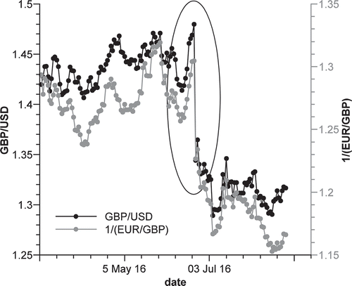
Reaction of exchange rates related to this anomaly was very strong: EUR/GBP growth 0.04650 points (max-min 0.07128), GBP/USD fall 0.1218 points (max-min 0.1659) in first day after voting; this trend continued for 9 days and then stabilized but did not return to previous levels even after 2 months.

The example cases indicate that the main reasons for the abnormalities in the currency market were natural or man-made: natural disasters, banking interventions, and geopolitical changes are only a few examples. Investors and speculators at the time, faced with the need to preserve investment, found ways to reduce losses or benefit from the huge fluctuations.

Prediction Model Based on Evolino RNN Ensemble

Prediction of exchange rates involves two different paradigms. The first paradigm states that future information is a continuation of past information. Many econometric techniques, such as moving averages and regression, are based on this approach. Can they predict the exchange rate variation anomalies? It is hardly possible. Furthermore, data anomalies affect the subsequent forecasts, even if the exchange rate quickly recovered. The second paradigm states, that future data can be chosen from a distribution of possibilities. We aim to combine these two approaches and to identify opportunities to recognize the upcoming anomaly, predict behavior of exchange rate during and after the time of anomaly, and reduce the risk of investment. The solution to this problem may be complex, combining forecasting based on artificial intelligence and the creation of portfolio using modern portfolio theory. The support system for the investor is shown in Figure 4. It consists of five steps:

Figure 4. Scheme of support system for investor based on ERNN ensemble.

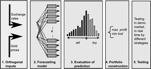
First step. Preparation of historical data. For the first input, we use historical data of exchange rates. What we want predict is: GBP/AUD, NZD/CAD, EUR/JPY, USD/CHF, EUR/USD, GBP/USD, USD/JPY. For the second input, we use historical data of gold prices in USD. The selection of which ranges of historical data to choose for this input was investigated by Maknickienė and Maknickas 2013). Prices of gold had not any anomalies when exchange rates had anomalies. The second input, like a “teacher” of neural networks, can not help to predict anomalies but can stabilize the accuracy of the prediction after the anomaly.

Second step. Forecasting. The model is based on EVolution of recurrent systems with Optimal LINear Output (Evolino), proposed by researchers Wierstra, Gomez, and Schmidhuber (2005) and Schmidhuber, Wierstra, and Gomez (2005). Our constructed forecasting model is an ensemble of 176 Evolino recurrent neural networks (ERNN). Each Evolino RNN uses two inputs, different historical data sets and predicts in one time, in parallel. Investigation of the prediction model is presented in papers by Maknickienė and Maknickas (2013); Maknickienė and Maknickas (2016). The result of the prediction is the distribution of the expected values.

Third step. Evaluation of the prediction. A multimodal distribution has a shape, mode value, and standard deviation. Calculation of profit and loss probabilities is generated according to the last known value or closing value of previous day. Some methods of evaluation of this combination of distributions were investigated in previous work: high-low strategy (Stankevičienė, Maknickienė, and Maknickas 2014); and UK-New York time zones (Maknickiene and Maknickas 2016). Investigation of distribution parameters before, at moment and after anomaly will be presented on the next section of the paper.

Fourth step. Portfolio constructing. The investment portfolio is composed in proportion to the probabilities of predicting profit.

Fifth step. Testing. Development of the support system, evaluation of predictions methods, and trading strategies are al examined via a real-time platform. This means that the efficiency, rationality of market, and psychology of investor are included in the testing of the prediction model. Support systems provide the additional information needed for decision-making in the finance market. Solutions of informed speculators have an advantage compared to the uninformed market participants.

Investigation of Exchange Market Anomalies

Our research compares two anomalies: the unexpected Swiss National Bank (SNB) intervention on 15 January 2015th and the expected vote of the British exit from the European Union (Brexit) on 23 June 2016. We prepared to explore the possible abnormality in two ways. First, do parameters of prediction by our support system reflect the foreign exchange market anomaly? Distribution of expected values has a shape of multimodal distribution. The most common mode is one, rarely two modes, even more rarely three or more modes. The standard deviation describes the riskiness of the decision. When standard deviation rises to 20% of its value, the trading decision is “too risky to trade.” Skewness and excess kurtosis indicate the closeness of the predicted distribution to a normal distribution. Mode I is the most likely predicted exchange rate value. Real max and min values help determine the predictive accuracy. Investigation of accuracy of prediction prior, during, and after an anomaly determines the dynamics of forecasting and the change in the reliability of the prediction. The second task investigates different portfolios. Which trading strategy is better for saving the investment during the significant changes of exchange rates? What opportunities arise for speculators due to the high exchange rate fluctuations?

Prediction by ERNN Ensemble

Our model, based on an ERNN ensemble, gives the distribution of expected values for the next day in New York time. It uses 2 years of historical data for calculating the prediction.

The Swiss National Bank (SNB) intervention, the Swiss francs decoupling from euro on 15 January, was an unexpected event for traders. Our daily trading in the exchange market allows for an assessment of the ERNN ensemble forecasting. The investigation interval is from 12 January 2015 to 23 January 2015. This includes 3 days before banking intervention, the day of SNB action, 2 days of maximal reaction, and 3 days after reaction. The exchange rates selected for the investigation are: USD/CHF; like rate of Switzerland and EUR/JPY; like rate related to the Euro. Table 1 presents the reaction of prediction of USD/CHF to SNB anomaly.

Table 1. Reaction of prediction of USD/CHF by ERNN ensemble to SNB anomaly.

	Before anomaly			During anomaly			After anomaly
Date	12 Jan	13 Jan	14 Jan	SNB	16 Jan	20 Jan	21 Jan	22 Jan	23 Jan
Shap	unimode	unimode	double	double	unimode	unimode	unimode	unimode	unimode
Stdev	0.009	0.003	0.006	0.009	0.009	1.63	error	18.74	3.34
Skewness	1.27	−0.23	1.39	0.05	1.45	1.4	error	1.7	0.95
Ex. Kurtosis	0.28	−1.5	0.5	−1.78	1.7	0.4	error	1.32	−0.93
Mode I	1.0135	1.015	1.016	1.026	1.025	0.9	0.9	0.9	0.9
Mode II			1.02	1.024
Real max	1.089	1.02173	1.02395	1.02198	0.88005	0.88307	0.87682	0.87462	0.88125
Real min	1.01175	1.01322	1.0137	0.83469	0.84462	0.86824	0.84974	0.85178	0.86873
Accuracy (%)	0.53	0.66	0.23	−0.39	−16.47	−1.9	−2.641	−2.9	−2.13

The forecast of 21 January was not used as the data exceeded the limits. Standard deviation from 20 to 23 January exceeds the exchange rate value threshold by 20% and trading using the ERNN ensemble becomes very risky. Losses in trading within the line of accuracy, labeled with a “minus” sign, began the first day of intervention. Accuracies of predictions significantly worsened from 16 of January and returned to the previous level only after 5 weeks. Prediction of EUR/JPY is presented in Table 2.

Table 2. Reaction of prediction of EUR/JPY by ERNN ensemble to SNB anomaly.

	Before anomaly			During anomaly			After anomaly
Date	12 Jan	13 Jan	14 Jan	SNB	16 Jan	20 Jan	21 Jan	22 Jan	23 Jan
Shape	3 modes	unimode	unimode	double	double	unimode	unimode	unimode	unimode
Stdev	4.87	8.78	0.43	6.44	51.16	29.32	error	5.26	25.98
Skewness	1.37	0.96	0.2	0.7	1.85	1.79	error	−0.15	1.7
Ex. Kurtosis	0.29	−0.37	−1.28	−1.4	1.7	1.54	error	−1.5	1.21
Mode I	140.5	140.5	141	138.5	139	134	134	138	138
Mode II	141/141.5			141.5	139
Real max	140.875	140.505	138.782	138.734	136.173	137.632	137.301	137.11	134.54
Real min	139.445	138.151	136.997	134.643	134.843	136.128	135.794	134.204	130.891
Accuracy (%)	0.27	3.5e-3	−1.6	2.87	−2.08	−1.56	−1.32	−0.65	−2.57

The extreme change in the exchange rate on 15th January impaired historical data and prediction such that data from 21 of January could not be used. Standard deviation arising from the first day of SNB intervention resulted in risky trading. The accuracy of prediction worsened 1 day before intervention.

The vote on the United Kingdom withdrawal from the European Union was not unexpected; therefore, it was possible to presume that the financial markets would react. As a result, we prepared to explore every possible abnormality carefully.

The investigation interval is from 20 June 2016 to 1 July 2016: 3 days before Brexit, voting day, day of maximal reaction, second day of reaction, and 3 days after reaction. Exchange rates, selected for investigation, are GBP/USD, GBP/AUD, like rates of UK and EUR/USD, and EUR/JPY like rates related to European Union (EU).

Table 3 presents predictions of GBP/USD by the ERNN ensemble to anomaly names Brexit. Parameters of the prediction distribution do not predict the anomaly on 24 June 2016. Differences in the shape of distribution were visible only on 27 June for 4 significant modes. The reaction, seen on data that showed big fluctuations, was influenced by the standard deviation of the original prediction from 27 June to 1 June and the accuracy of the prediction from 27 to 29 June. Table 3 presents predictions of GBP/USD by ERNN ensemble to anomaly names Brexit.

Table 3. Reaction of prediction of GBP/USD by ERNN ensemble to “Brexit” anomaly.

	Before anomaly			During anomaly			After anomaly
Date	20 Jun	21 Jun	22 Jun	Brexit	24 Jun	27 Jun	29 Jun	30 Jun	1 Jul
Shape	unimode	double	double	unimode	unimode	4modes	unimode	double	double
Stdev	0.02	0.07	0.05	0.05	0.09	1.31	0.3	0.26	0.21
Skewness	−0.5	3.76	−1.47	1.7	3.35	2.84	1.16	1.1	−0.3
Ex. Kurtosis	1.29	24.78	3.97	5.91	20	9.69	6.03	7.04	1.75
Mode I	1.46	1.48	1.47	1.49	1.51	1.	1.3	1.35	1.35
Mode II		1.465	1.48			1.2		1.4	1.3
Real max	1.472	1.4784	1.4774	1.4947	1.5019	1.3672	1.342	1.3533	1.3496
Real min	1.4357	1.4619	1.4642	1.4707	1.3228	1.3119	1.3202	1.3287	1.3206
Accuracy (%)	0.82	−0.1	0.5	0.3	0.1	−26	−3.1	0.2	0.2

Prediction distribution parameters do not predict anomalies on 24 June 2016. Differences in the shape of distribution were visible only on 27 June for 4 significant modes. The reaction, seen on data that showed big fluctuations, was influenced by the standard deviation of the original prediction from 27 June to 1 June and the accuracy of the prediction from 27 to 29 June.

Table 4 presents data of GBP/AUD predictions for 20 June–1 July. Standard deviation changed only after Brexit fluctuations from 27 June. The accuracy of prediction fell from 24 June.

Table 4. Reaction of prediction of GBP/AUD by ERNN ensemble to “Brexit” anomaly.

	Before anomaly			During anomaly			After anomaly
Date	20 Jun	21 Jun	22 Jun	Brexit	24 Jun	27 Jun	29 Jun	30 Jun	1 Jul
Shape	double	double	unimode	double	double	double	unimode	double	double
Stdev	0.09	0.08	0.06	0.08	0.05	0.31	0.17	0.19	0.12
Skewness	−0.38	0.68	−0.61	1.17	0.03	2.26	−0.07	0.28	−0.72
Ex. Kurtosis	3.87	3.18	1.11	7.78	2.67	12.96	4.45	3.51	1.71
Mode I	1.93	1.92	1.96	1.96	1.96	1.8	1.75	1.8	1.75
Mode II	1.9	1.9		1.98	1.94	1.7		1.75	1.8
Real max	1.9447	1.9738	1.9717	1.9729	1.9676	1.8312	1.8192	1.8181	1.7937
Real min.	1.9263	1.9417	1.9466	1.8017	1.777	1.7944	1	1.7756	1.7692
Accuracy (%)	0.7	−1.1	0.4	0.7	8.8	1.3	2.5	1.4	−1

EUR/USD prediction parameters are presented in Table 5. Reaction of EUR/USD to the Brexit anomaly is minimal: only standard deviation and accuracy on 27 June is extremely more than usual.

Table 5. Reaction of prediction of EUR/USD by ERNN ensemble to “Brexit” anomaly.

	Before anomaly			During anomaly			After anomaly
Date	20 Jun	21 Jun	22 Jun	Brexit	24 Jun	27 Jun	29 Jun	30 Jun	31Jul
Shape (modes	unimode	unimode	unimode	unimode	double	unimode	double	double	double
Stdev	0.04	0.008	0.007	0.007	0.0008	0.39	0.04	0.05	0.03
Skewness	0.39	0.31	0.14	0.46	0.63	2.31	0.97	−3.11	0.68
Ex. Kurtosis	3.39	0.26	1.02	0.49	1.37	7.7	2.54	18.46	4.3
Mode I	1.115	1.14	1.13	1.15	1.14	1.05	1.1	1.12	1.11
Mode II		1.35			1.135		1.12	1.11	1.1
Real max	1.1382	1.1349	1.1337	1.421	1.1428	1.1108	1.113	1.1154	1.1169
Real min	1.1276	1.1242	1.1236	1.1296	1.0911	1.097	1.1049	1.1024	1.1072
Accuracy (%)	−1.1	−0.5	0.3	0.7	0.2	−5.5	0.4	−0.4	0.6

Table 6 presents predictions of EUR/JPY before, during, and after the Brexit anomaly. The shape of the distribution of expected values was extremely different on the day of voting for Brexit (24 June). Reaction of prediction parameters was also delayed. Standard deviation increased and accuracy fell beginning 27 June.

Table 6. Reaction of prediction of EUR/JPY by ERNN ensemble to “Brexit” anomaly.

	Before anomaly			During anomaly			After anomaly
Date	20 Jun	21 Jun	22 Jun	Brexit	24 Jun	27 Jun	29 Jun	30 Jun	1 Jul
Shape	unimode	unimode	double	4 modes	unimode	unimode	unimode	unimode	unimode
Stdev	0.9	1.05	1.2	1.4	1.3	19.6	15.78	20.24	11.93
Skewness	0.19	−0.53	0.66	0.41	−0.39	3.97	0.5	3.29	1.14
Ex. Kurtosis	0.48	2.23	1.46	1.83	1.14	23.87	2.76	14.37	5.54
Mode I	118	116.5	117.5	118.5	119	110	110	110	110
Mode II			118	115
Real max	118.1	119.14	118.61	120.94	122.01	113.51	114.5	114.79	114.73
Real min	116.9	117.35	117.42	117.93	109.57	111.38	112.94	113.34	113.68
Accuracy (%)	0.9	−0.7	0.9	0.5	0.9	−1.2	−2.6	−2.9	−3.2

Predictions by the ERNN ensemble before Brexit are like the usual predictions during normal trading. Only one very high excess kurtosis value was observed on 21 June, GBP/USD. On the day before the vote, for the British exit from EU, had no reaction in market or in predicting. The market had an extreme reaction as a result of the vote, but our predictions by ERNN ensemble were without reaction. Accuracy fell only for GBP/AUD prediction, but direction of change of exchange rate was predicted correctly, so profits were made, although not as large as in the exchange rate fell down. Fluctuations of exchange rates on the next day (27 June) were large. Predictions by the ERNN ensemble show extreme changes in standard deviation, accuracy of prediction, and excess kurtosis. This reaction was influenced by the extreme change of data (24 June), used for prediction, and remained long after the anomaly: GBP/USD, GBP/AUD, EUR/JPY from 27 June to 26 July, EUR/USD did not react.

Comparison of two anomalies shows that the prediction model based on ERNN ensemble is balanced for daily and weekly trade in the currency market and does not alert the investor about the anomalies which occurs very rarely. On the day of the anomaly can be very unprofitable for long time investors but not extremely dangerous for daily speculators, if they use the protections. Period after anomaly is very risky, because historical data, using by ERNN ensemble, are messed up.

Comparison of Trading Strategies

SNB intervention was an unexpected anomaly. We had daily trading in real-time demo trading platform by four exchange rates: GBP/AUD, NZD/CAD, EUR/JPY, and USD/CHF. Three strategies were tested: conservative, where assets are divided equally, moderate, where assets are distributed in proportion to the probability of profit, determined from the prediction distribution, and aggressive strategy, where asset is allocating only in two exchange rate with maximal predicted profit. The results of trading in period from 12th January 2015 to 26 January 2015 are shown in Figure 6.

Figure 5. Trading in time of SNB intervention by tree different strategies.

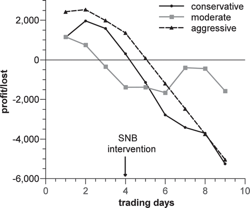
All three trading strategies had losses induced by the anomaly named SNB intervention. After intervention, conservative and aggressive strategies continued to generate losses during trading. The moderate strategy had stable losses. Any continuation of losses, after intervention, was determined by abnormal historical data used in the calculation of prediction by the ERNN ensemble. The forecast, with a standard deviation that exceeded 20% of the exchange rate value, is not reliable. A real market speculator who would not trade for some time and wait until the forecasts became credible once again is sensible.

The investigation of an investor’s ability to save investments or profit from large exchange rate fluctuations is made by constructing different portfolios and testing them. The first portfolio is constructed from exchange rates related to GBP end EUR, its name is “related.” The second portfolio is called “not related” and it is constructed without GBP and EUR. The anomaly can be unexpected, so orthogonal and not orthogonal portfolios will be investigated as a result. Roll (1980) first introduced the term “orthogonal portfolio.” An orthogonal portfolio satisfies the equation: Σσ_iσ_jρ_ij = 0 where σ is standard deviation (STDEV) of i or j exchange rate, ρ_ij is correlation coefficient of i and j exchange rates. Correlation coefficients and standard deviations are shown in Table 7.

Table 7. Correlations and STDEV of exchange rates.

	GBP/AUD	NZD/CAD	EUR/JPY	USD/CHF	EUR/USD	GBP/USD	USD/JPY
GBP/AUD	1	−0.465	0.07	0.34	−0.6	−0.01	0.72
NZD/CAD	−0.465	1	−0.26	−0.02	0.006	−0.24	−0.25
EUR/JPY	0.07	−0.26	1	−0.3	0.52	0.81	0.43
USD/CHF	0.34	−0.02	−0.3	1	−0.52	−0.54	0.26
EUR/USD	−0.6	0.006	0.52	−0.52	1	0.68	−0.54
GBP/USD	−0.01	−0.24	0.81	−0.54	0.68	1	0.1
USD/JPY	0.72	−0.25	0.43	0.26	−0.54	0.1	1
STDEV	0.123	0.03	751	0.03	0.02	0.08	6.72

Since zero in the calculation of orthogonality is hard to reach, Σσiσjρij = ε is calculated as a measure of the proximity to orthogonality (Table 8).

Table 8. Orthogonality of portfolios.

Portfolio	Rates	ε
Related	GBP/AUD;GBP/USD;EUR/JPY;EUR/USD	0.63
Not related	NZD/CAD;USD/CHF;EUR/USD;USD/JPY	0.05
Orthogonal	NZD/CAD;USD/CHF;EUR/USD;GBP/USD	−0.001
Not orthogonal	EUR/JPY;USD/JPY;GBP/AUD;GBP/USD	22.90

The four portfolios were tested in a demo market. Three days before the Brexit vote were simple days for trading. Next, we use the voting day without market reaction and the two second days with highest fluctuations. The next 3 days had lower fluctuations, but historical data used for calculating the prediction reacted to anomalies of the exchange rates, as a result, the prediction is not accurate. “Take profit” is the label for the mode of distribution of expected values; profit depends on the prediction. “Stop loss” is the label for the STDEV of the exchange rate; the risk of losing all assets as a result of an anomaly is not high.

The first strategy for comparing the four portfolios is conservative; asset allocation is equal for each currency pair. The second strategy is moderate; assets are distributed in proportion to the probabilities defined by the distributions of expected values. The third strategy is aggressive and is therefore more risky; assets are distributed only in the two exchange rates with the highest expectations.

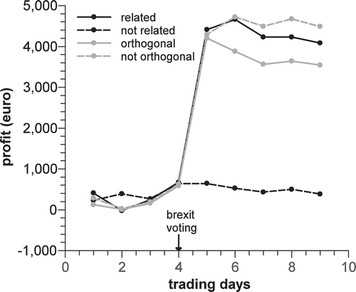
Comparison of related and unrelated Brexit portfolios is shown in Figure 7 using a black line and dotted line, respectively. Portfolios that are or are not orthogonal are shown in Figure 7 using a gray line and dotted line, respectively. The results show that unrelated portfolios are unable to win on the big exchange rate fluctuations since its profit line did not react to the anomaly. The other three portfolios demonstrate a huge leap caused by the significant fluctuations in exchange rates immediately after the vote Brexit. Later, profit slowly declined as forecasts become inaccurate due to the distortion of the historical data.

Figure 6. Trading by conservative strategy.

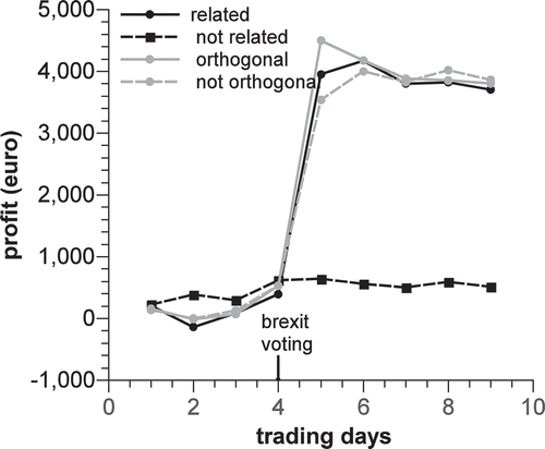
The comparison of four portfolios using the moderate strategy is presented in Figure 8. The portfolios that were unrelated to the anomaly had usual fluctuation of profit. Three other portfolios showed huge leaps on the day after voting: the highest was the orthogonal case, the next highest was the related case and finally the data that was not orthogonal showed the next highest returns. After the anomaly, three lines became close.

Figure 7. Trading by moderate strategy.

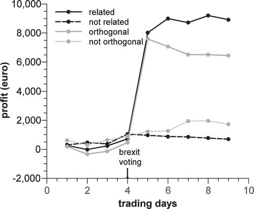
The aggressive strategy had the highest risk but also the highest opportunity for profit (Figure 9). Trading for the unrelated and not orthogonal portfolios did not react to the anomaly or profit from one exchange rate as it was compensated by the loss of the other. The related portfolio experienced a huge leap on the next day after highest fluctuation and preserved achievements for the next 3 days. Orthogonal portfolios had high leap of profit too, but after the line of profit declined.

Figure 8. Trading by aggressive strategy.

The anomaly in the currency market offers great opportunities for speculators in the short run and great risk for long-term investment. Anomalies can be expected and unexpected. If speculator has information about opportunity of anomaly, it is appropriate to trade in foreign exchange rates related to the anomaly. If the anomaly is unexpected, trading success depends on the accuracy of forecasts and on the sets of exchange rates linked with the anomaly.

Conclusions

An anomaly in the exchange rate market happens from time to time; as a result, it is important to investigate the trading strategies during those periods of time. The time during an anomaly is an important moment of market time. This happens when the future predictions are not determined by a sequential continuation of the past. In this case, models perform better if predictions are based on probabilities or distributions of possibilities. The prediction model based on the ERNN ensemble is balanced for daily and weekly trades in the exchange market. The result of the prediction is found via a distribution of expected values. Probability of extreme values is not zero; as a result, an investor must be ready for anomalies.

Parameters for predicting distributions do not alert the investor about the anomalies. Reaction to the anomaly was visible only after the anomaly, and only when model began to use data influenced by extreme change. Standard deviation increased to 6247 times. The accuracy of the prediction after the anomaly fell to 130 times.

An unexpected anomaly in the currency market is marked by random success or failure, depending on the selected exchange rate relationship with the anomaly. The periods after the anomaly are very risky. This is because of the reliability of forecasts which are conditioned by confused historical data.

Investment portfolios can not only reduce risk and protect investments through asset allocation, but also provide additional opportunities for speculators. In this work, we compared four different portfolios: related to the anomaly, not related to the anomaly, orthogonal, and not orthogonal. By analyzing the conservative, moderate and aggressive portfolios we see that, in the moment of the anomaly profit, speculation depends on accuracy of prediction and on the sets of exchange rate linked to the anomaly.

Results show that the anomaly created by the United Kingdom (UK) vote to withdraw from the European Union (EU), gives the best opportunity for speculator. Trading using the ERNN ensemble model allows the profit to increase from 1.8% to 8.9% for 6 trading days, for portfolios related to Brexit, and 0.3–0.6%, for portfolios not related to the anomaly.

Conservative and moderate strategies yield approximately equal opportunities for all related to anomaly strategies. Aggressive strategies can yield twice the profit for orthogonal portfolios and portfolios with a link to the anomaly. A non-orthogonal portfolio did not react to anomaly.

References

- Acharya, N., N. A. Shrivastava, B. Panigrahi, and U. Mohanty. 2014. Development of an artificial neural network based multi-model ensemble to estimate the northeast monsoon rainfall over south peninsular india: An application of extreme learning machine. Climate Dynamics 43 (5–6):1303–10. doi:10.1007/s00382-013-1942-2.
- Ahmed, M., A. N. Mahmood, and M. R. Islam. 2016. A survey of anomaly detection techniques in financial domain. Future Generation Computer Systems 55:278–88. doi:10.1016/j.future.2015.01.001.
- Avramov, D., and T. Chordia. 2006. Asset pricing models and financial market anomalies. Review of Financial Studies 19 (3):1001–40. doi:10.1093/rfs/hhj025.
- Bouchaud, J. P., P. Krueger, A. Landier, and D. Thesmar 2016 Sticky expectations and stock market anomalies. HEC Paris Research Paper.
- Cella, C., A. Ellul, and M. Giannetti. 2013. Investors’ horizons and the amplification of market shocks. Review of Financial Studies 26 (7):1607–48. doi:10.1093/rfs/hht023.
- Chu, Y., D. A. Hirshleifer, and L. Ma. 2015. The causal effect of limits to arbitrage on asset pricing anomalies. Available at SSRN.
- Gupta, A., M. Kumar, and S. Kumar.2016. A novel approach for market prediction using differential evolution and genetic algorithm. Proceedings of Fifth International Conference on Soft Computing for Problem Solving, Springer, Singapore, 377–90
- Israel, R., and T. J. Moskowitz. 2013. The role of shorting, firm size, and time on market anomalies. Journal of Financial Economics 108 (2):275–301. doi:10.1016/j.jfineco.2012.11.005.
- Jones, C. S., and L. Pomorski.2016. Investing in disappearing anomalies. Review of Finance, rfv065
- Kontonikas, A., and A. Kostakis. 2013. On monetary policy and stock market anomalies. Journal of Business Finance & Accounting 40 (7–8):1009–42. doi:10.1111/jbfa.12028.
- Kvietkauskienė, K., and N. Maknickienė. 2015. The use of investment portfolio orthogo- nality to secure investment against bank interventions. Journal of System and Management Sciences (JSMS) 5 (3):1–17.
- Lamont, O. A., and R. H. Thaler. 2003. Anomalies: The law of one price in financial markets. The Journal of Economic Perspectives 17 (4):191–202. doi:10.1257/089533003772034952.
- Li, J., and N. C. Miller. 2015. Foreign exchange market inefficiency and exchange rate anomalies. Journal of International Financial Markets, Institutions and Money 34:311–20. doi:10.1016/j.intfin.2014.12.001.
- Maghrebi, N., M. J. Holmes, and K. Oya. 2014. Financial instability and the short-term dynamics of volatility expectations. Applied Financial Economics 24 (6):377–95. doi:10.1080/09603107.2014.881966.
- Maknickiene, N., and A. Maknickas 2016. Impact of time zones on forecasting of exchange market based on distribution of expected values. The 9th International Scientific Conference Business and Management 2016, May 12 –13,2016, Vilnius, Technika, 1–8
- Maknickienė, N., and A. Maknickas. 2013. Financial market prediction system with evolino neural network and delphi method. Journal of Business Economics and Management 14 (2):403–13. doi:10.3846/16111699.2012.729532.
- Maknickienė, N., and A. Maknickas. 2016. Prediction capabilities of evolino rnn ensembles. In Madani K., Dourado A., Rosa A., Filipe J., Kacprzyk J. (eds.), Computational Intelligence. Studies in Computational Intelligence, vol 613. Springer, Cham.
- Malhotra, P., L. Vig, G. Shroff, and P. Agarwal. 2015. Long short term memory networks for anomaly detection in time series. Proceedings on European Symposium on Artificial Neural Networks, Computational Intelligence and Machine Learning. Bruges (Belgium), 22-24 April 2015, Presses universitaires de Louvain, 89–94
- Namazi, M., A. Shokrolahi, and M. S. Maharluie. 2016. Detecting and ranking cash flow risk factors via artificial neural networks technique. Journal of Business Research 69 (5):1801–06. doi:10.1016/j.jbusres.2015.10.059.
- Novy-Marx, R. 2013. The other side of value: The gross profitability premium. Journal of Financial Economics 108 (1):1–28. doi:10.1016/j.jfineco.2013.01.003.
- Novy-Marx, R., and M. Velikov. 2016. A taxonomy of anomalies and their trading costs. Review of Financial Studies 29 (1):104–47. doi:10.1093/rfs/hhv063.
- Roll, R. 1980. Orthogonal portfolios. Journal of Financial and Quantitative Analysis 15 (5):1005–23. doi:10.2307/2330169.
- Schmidhuber, J., D. Wierstra, and F. Gomez 2005. Evolino: Hybrid neuroevolution/optimal linear search for sequence learning. Proceedings of the 19th international joint conference on Artificial intelligence, Morgan Kaufmann Publishers Inc., Edinburgh, 853–58.
- Schwert, G. W. 2003. Anomalies and market efficiency. Handbook of the Economics of Finance 1:939–74.
- Shu, H. C., and J. H. Chang. 2015. Investor sentiment and financial market volatility. Journal of Behavioral Finance 16 (3):206–19. doi:10.1080/15427560.2015.1064930.
- Stambaugh, R. F., J. Yu, and Y. Yuan. 2012. The short of it: Investor sentiment and anomalies. Journal of Financial Economics 104 (2):288–302. doi:10.1016/j.jfineco.2011.12.001.
- Stankevičienė, J., N. Maknickienė, and A. Maknickas 2014. Investigation of exchange market prediction model based on high-low daily data. In: Proceedings of the 8th international scientific conference ”Business and Management 2014”: selected papers. May 15-16, 2014, Vilnius, Technika, 320–27
- Subrahmanyam, A., and S. Titman. 2013. Financial market shocks and the macroeconomy. Review of Financial Studies 26 (11):2687–717. doi:10.1093/rfs/hht058.
- Ter Ellen, S., W. F. Verschoor, and R. C. Zwinkels. 2013. Dynamic expectation formation in the foreign exchange market. Journal of International Money and Finance 37:75–97. doi:10.1016/j.jimonfin.2013.06.001.
- Wierstra, D., F. J. Gomez, and J. Schmidhuber 2005. Modelling systems with internal state using evolino. Proceedings of the 7th annual conference on Genetic and evolutionary computation, ACM, Munich, Germany. 1795–802
- Yalcin, K. C. 2016. Market rationality: Efficient market hypothesis versus market anomalies. European Journal of Economic and Political Studies 3 (2):23–38.
- Zafari, F., G. M. Khan, M. Rehman, and S. Ali Mahmud. 2014. Evolving recurrent neural network using cartesian genetic programming to predict the trend in foreign currency exchange rates. Applied Artificial Intelligence 28 (6):597–628.