Bi-direction Direct RGB-D Visual Odometry

ABSTRACT

Direct visual odometry (DVO) is an important vision task which aims to obtain the camera motion via minimizing the photometric error across the different correlated images. However, the previous research on DVO rarely considered the motion bias and only calculated using single direction, therefore potentially ignoring useful information compared with leveraging diverse directions. We assume that jointly considering forward and backward calculation can improve the accuracy of pose estimation. To verify our assumption and solid this contribution, in this paper, we test various combination of direct dense methods, including different error metrics, e.g., (intensity, gradient magnitude), alignment strategies (Forward-Compositional, Inverse-Compositional), and calculation directions (forward, backward, and bi-direction). We further study the issue of motion bias in RGB-D visual odometry and propose four strategy options to improve pose estimation accuracy, e.g., joint bi-direction estimation; two stage bi-direction estimation; transform average with weights; and transform fusion with covariance. We demonstrate the effectiveness and efficiency of our proposed algorithms across a range of popular datasets, e.g., TUM RGB-D and ICL-NUIM, in which we achieve an impressive performance through comparing with state of the art methods and provide benefits for existing RGB-D visual odometry and visual SLAM systems.

Introduction

Visual simultaneous localization and mapping (vSLAM) and visual odometry (VO) are the important tasks in computer vision and robotics community. VO can be considered as a subproblem of vSLAM and focuses on estimating the relative motion between consecutive image frames. In addition to monocular (Lin et al. 2018) and stereo cameras (Cvišic et al. 2017; Ling and Shen 2019), in recent years, visual odometry with RGB-D sensors has gained superior attentions in various research aspects (Zhou, Li, and Kneip 2018) and successfully applied to unmanned aerial vehicle (Iacono and Sgorbissa 2018), autonomous ground vehicle (Aguilar et al. 2017a), augmented reality, and virtual reality (Aguilar et al., 2017b).

RGB-D camera provides a simple yet cost-effective way to obtain RGB and additional depth information of scene (Dos Reis et al. 2019). Similar as traditional visual odometry, RGB-D visual odometry can also be divided into feature-based methods and direct methods. Feature-based methods require feature extraction and data association. However, these methods achieve poor performance within textureless conditions. In contrast, direct methods optimize the rigid-body transformation between two frames by minimizing the photometric error. They have been shown to be more robust against image blur. Recent research also shows that direct methods present higher accuracy than feature-based methods both in odometry (Engel, Koltun, and Cremers 2017) and mapping (Schops, Sattler, and Pollefeys 2019; Zubizarreta, Aguinaga, and Montiel 2020). By introducing camera internal parameters and exposure parameters into the photometric model as optimization variables, the front-end odometry results are improved. The back-end mapping part based on the photometric bundle adjustment can also benefit from the informative reobservations by the proposed persistent map (Zubizarreta, Aguinaga, and Montiel 2020).

The substantial drift caused by inaccurate frame-to-frame ego-motion is the main challenge for long-term direct visual odometry. As a common knowledge, the basic idea of direct image alignment adopts the formulation of the well known Lucas-Kanade approach (Baker and Matthews 2004). Proesmansl et al. found that the forward and backward scheme of the optical flow are not equivalent due to the large inconsistencies near edges and occluding regions. In (Proesmans et al. 1994), they proposed a dual optical flow scheme to measure the inconsistency. Forward-backward consistency check can also be used to eliminate false matches in feature tracking element of the stereo visual odometry (Deigmoeller and Eggert 2016) and monocular vision odometry (Bergmann, Wang, and Cremers 2017). Additionally, this idea has also gained much popularities in the recent deep learning-based optical flow estimation problem (Pillai and Leonard 2017). The motion estimation was refined by filtering some occluded and overshifted pixels (Hu, Song, and Li 2016; Revaud et al. 2015; Yin and Shi 2018). However, direct method is essentially derived from optical flow method, whereas the current direct methods merely consider forward calculation.

Inspired by the important concept “dataset motion bias” raised in reference (Engel, Usenko, and Cremers 2016) which proposed a VO/SLAM algorithm using different strategies, e.g., forward and backward, whereas the performances were obtained differently, the objective of this paper is to enhance the accuracy of odometry estimation by jointly considering forward and backward estimation. Through detailed discussion, Yang et al. introduced a convincing reason about “motion bias” (Yang et al. 2018), while the experimental results showed that feature-based methods, such as ORB-SLAM (Mur-Artal and Tardós 2017), perform significantly better for backward-motion, whereas the direct methods, such as DSO (Engel, Koltun, and Cremers 2017) achieve slight influence. In response, they claimed that the feature which nearby camera improves depth estimates when moving backward. The summarized rationales drove the developments of sparse monocular VO algorithm proposed by Pereira (Pereira et al. 2017), in which images are processed in reverse order. Besides, there are limited references further exploring the concept of motion bias.

The quality of depth estimation by triangulation is an important factor of motion bias in monocular VO. In contrast, in RGB-D VO, the quality of the depth data is sensitive to the variations of viewpoints, object materials and measure distances. Using the depth map of the current frame or the reference frame to calculate the 3D point cloud in the alignment part will also lead to different estimation results. Therefore, there is a potential possibility of motion bias in RGB-D visual odometry.

Figure 1. The flow chart of the proposed bi-direction motion estimation

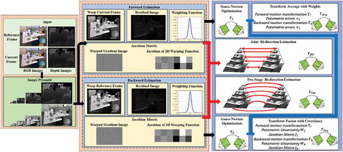
The purpose of this paper is to verify the forward-backward inconsistency characteristics in RGB-D direct frame alignment. As shown in Figure 1, we innovatively introduce the idea of motion bias to refine frame-to-frame motion estimation in direct RGB-D visual odometry. Our main contributions are summarized as follows:

(1) We deeply explore the issue of motion bias in RGB-D frame-to-frame motion estimation with the TUM RGB-D and ICL-NUIM datasets. We demonstrate that the reason of the inconsistency is the different quality of the depth data in current frame and reference frame. The forward and backward iterative calculations will lead to positive and negative bias, which can significantly improve the accuracy.

(2) We propose four strategy options to improve pose estimation accuracy: tight coupling (joint bi-direction estimation and two stage bi-direction estimation) and loose coupling (transform average with weights and transform fusion with covariance) for a thoughtful comparison. Results show that two stage bi-direction estimation achieves the best performance both on speed and accuracy.

(3) We carry out extensive experiments with different combined methods (e.g., Intensity or Gradient Magnitude, Forward Compositional or Inverse Compositional, Single Direction or Bi-direction) on the benchmark datasets to demonstrate the effectiveness of our solution.

The rest of this paper is organized as follows: Section II introduces the current research w.r.t the research field of direct RGB-D visual odometry. The whole framework is discussed in Section III. Section IV clearly introduces the experiment condition and evaluates the results of experiments in ICL-NUIM and TUM RGB-D benchmark sequences. Finally, whole research and the future work are summarized in Section V.

Related Work

There are extensive literatures related with research on RGB-D visual odometry (Civera and Lee 2019). In this section, our research attention is mainly focused on direct frame alignment-based approaches. Additionally, some methods related to the motion bias or forward-backward consistency are also be introduced.

Direct Frame Alignment

As a representative research, Kerl et al. (Kerl, Sturm, and Cremers 2013) introduced a Bayesian framework based Direct visual odometry (DVO) method, which estimated the camera motion between consecutive frames by minimizing the photometric error directly. It is worth noting that, Kerl (Kerl, Sturm, and Cremers 2013) also leveraged the merits of motion prior and robust error function for further improving the method. Klose et al. introduced different alignment strategy in optical flow method to direct RGB-D visual odometry, thus generating different methods, e.g., Forward Compositional (FC), Inverse Compositional (IC), and Efficient Second-order Minimization (ESM) (Klose, Heise, and Knoll 2013). Following the previous research, Babu (Babu et al. 2016) proposed a method, which novelly proposed additional probabilistic sensor noise model for geometric errors rather than considering t-distribution for optimizing photometric errors solely. Similar research in (Wasenmüller, Ansari, and Stricker 2016) leveraged the local depth derivatives to measure the reliability and transformed that into a weighting scheme which significantly reduced the drift.

Direct frame alignment algorithms rely on the photometric constancy assumption, which is not satisfied for real applications. In DSO (Engel, Koltun, and Cremers 2017), the photometric calibration model was used for complex lighting scene. In addition, several research considered other robust metric functions. Alismail et al. leveraged the squared distance between local feature descriptors instead of photometric error which shrinked the requirements for illumination modeling (Alismail, Browning, and Lucey 2016). Compared with raw intensity values, edges are more stable in scenes with varying light conditions, in which the photoconsistency-based approaches generally failed. Kuse and Shen proposed a novel direct approach which optimized the geometric distances of edge-pixels instead of photometric error (Kuse and Shen 2016). Schenk and Fraundorfer also introduced a robust edge-based visual odometry system by jointly minimizing edge distance and point-to-plane error (Schenk and Fraundorfer 2017a) for RGB-D sensors and extend it into a complete SLAM system (Schenk and Fraundorfer 2019). Zhou et al. proposed more efficient distance field methods for real-time edge alignment without losing accuracy and robust (Zhou, Li, and Kneip 2018).

However, the mentioned methods merely consider the forward direction from reference frame to current frame, which ignores the bi-directional strategies. To improve the defect about the single-direction strategy, our research explores the backward motion and introduces bi-direction estimation for improving the accuracy of the odometry.

Forward-backward Consistency and Motion Bias

The transitivity of regularize structured data can be categorized into forward-backward consistency or cycle consistency. Some current research are trying to exploit the merits about the forward-backward consistency. In current research, the pose consistency is incorporated into loss function to enforce forward-backward motion (Wong et al. 2020). In dense semantic alignment, Zhou et al. (Zhou et al. 2016) used a cycle consistency loss to supervise convolutional neural network training. In monocular visual odometry, Wong et al. employed bi-directional convolution LSTM (Bi-ConvLSTM) for learning the geometric relationship from image sequences pre and post and leveraged optical flow prediction to assist pose estimation (Wan, Gao, and Wu 2019).

For visual odometry, the intuitive sense about estimated trajectory should be the same despite the running algorithms on a sequence forward or backward. It is interesting to note that, recent research shows that different algorithms achieve different performances on a same data set which named as motion bias (Yang et al. 2018). Pereira et al. took advantage of backward movement in feature-based monocular visual odometry. Sparse features moving away from the camera can improve both depth calculation precision and pose estimation robustness.

As we know, the depth map acquired by Kinect contains quite an amount of holes and the depth values on the edges suffer from big error. To overcome the shortcoming that single direction calculation using only one depth map, in our research, we introduce a similar idea to direct motion estimation with forward-backward for offsetting each other.

Direct Motion Estimation

In this section, we introduce the proposed approach, namely the direct RGB-D visual odometry. First, we formulate the problem as a nonlinear least square minimization (Section 3.1). Then, we present a error metric function by gradient magnitude to deal with the challenge of illumination variation (Section 3.2). Finally, we propose four methods to incorporate the motion information using bi-direction (Section 3.3 and Section 3.4) for detail exploration.

Overview

Similar as in (Kerl, Sturm, and Cremers 2013), our goal is to estimate the RGB-D camera motion between a reference frame and the current frame. We assume the intensity image and the depth map at each timestamp to be synchronized and aligned, therefore a pixel ${\mathbf{x}}_i=(u_i,v_i{)}^T$ in image space $\mathrm{\Omega }\in {\mathbb{R}}^2$ is corresponded to the depth $Z\left({\mathbf{x}}_i\right)$. The 3D point ${\mathbf{P}}_i=(X_i,Y_i,Z_i{)}^T$ is related to the pixel ${\mathbf{x}}_i$, which is computed by the inverse of the projection function $\pi$ as:

(1) ${\mathbf{P}}_i={\pi }^{-1}({\mathbf{x}}_i,Z_i)=Z_i{\left(\frac{u_i-c_x}{f_x},\frac{v_i-c_y}{f_x},1\right)}^T$(1)

in which $(c_x,c_y)$ is the principal point of camera, and $(f_x,f_y)$ is the focal length. $Z_i$ is equal to the depth measurement $Z\left({\mathbf{x}}_i\right)$. Similarly, the projection function is given as:

(2) ${\mathbf{x}}_{\mathbf{i}}=\pi \left({\mathbf{P}}_i\right)=\left(\frac{X_i{f}_x}{Z_i}+c_x,\frac{Y_i{f}_y}{Z_i}+c_y\right)$(2)

Let $\mathbf{T}=\left(\mathbf{R},\mathbf{t}\right)\in SE(3)$ denotes a rigid transformation between the two views, where $\mathbf{R}\in SO(3)$ and $\mathbf{t}\in {\mathbb{R}}^3$ represent rotation and translation respectively. Since the rotation matrix has constraints, i.e., $\mathbf{R}{\mathbf{R}}^T=\mathbf{I},det\left(\mathbf{R}\right)=1$, we use the Lie algebra $se(3)$ to parameterize the transformation as a twist coordinates $\xi =\left(\mathbf{v},\omega \right)$. $\mathbf{v}$ is linear velocity, and $\omega$ is the angular velocity of the motion. For a given parameter vector $\xi$, the corresponding $4\times 4$ transformation matrix can be retrieved with the exponential map:

(3) $\mathbf{T}\left(\xi \right)=exp\left(\left[\begin{array}{cc}{\omega }^{\wedge }& \mathbf{v}\\ {\mathbf{0}}^T& 0\end{array}\right]\right)$(3)

where ${\omega }^{\wedge }$ denotes the skew symmetric matrix of the angular vector $\omega$. Then the full warping function is defined as:

(4) $\begin{array}{cc}\tau \left(\xi ,{\mathbf{x}}_i,Z\left({\mathbf{x}}_i\right)\right)& =\pi \left({\left(\mathbf{T}\left(\xi \right)\left[\begin{array}{c}{\mathbf{P}}_i\\ 1\end{array}\right]\right)}_{1:3}\right)\\ \hspace{0.17em}& =\pi \left({\left(\mathbf{T}\left(\xi \right)\left[\begin{array}{c}{\pi }^{-1}\left({\mathbf{x}}_i,Z\left({\mathbf{x}}_i\right)\right)\\ 1\end{array}\right]\right)}_{1:3}\right)\end{array}$(4)

where ${\left(\hspace{0.17em}\right)}_{1:3}$ indexes the first three elements of the vector. The direct visual odometry estimates the motion $\xi$ by minimizing the photometric errors between the reference frame ${\mathbf{I}}_r$ and the current frame ${\mathbf{I}}_c$ as:

(5) $E=\underset{\xi }{min}\sum _{{\mathbf{x}}_i\in \mathrm{\Omega }}{\left({\mathbf{I}}_c\left(\tau \left(\xi ,{\mathbf{x}}_i,Z\left({\mathbf{x}}_i\right)\right)\right)-{\mathbf{I}}_r\left({\mathbf{x}}_i\right)\right)}^2$(5)

The above problem is a nonlinear least square problem and can be solved by Gauss-Newton algorithm. The motion estimation $\mathbf{T}\left(\xi \right)$ is updated by increment $\mathrm{\Delta }\xi =-({\mathbf{J}}^T\mathbf{J}{)}^{-1}{\mathbf{J}}^T\mathbf{r}$ until convergence: $\mathbf{T}\left(\xi \right)\leftarrow \mathbf{T}\left(\xi \right)\mathbf{T}\left(\mathrm{\Delta }\xi \right)$, where $\mathbf{J}$ is the stacked matrix of all ${\mathbf{J}}_i$ pixel-wise Jacobians and $\mathbf{r}$ denotes the residual vector. According to the chain rule, ${\mathbf{J}}_i$ is given by:

(6) ${\mathbf{J}}_i=\frac{\mathrm{\partial }{r}_i}{\mathrm{\partial }\mathbf{x}}=\frac{\mathrm{\partial }{\mathbf{I}}_c}{\mathrm{\partial }{\mathbf{x}}_i}\frac{\mathrm{\partial }{\mathbf{x}}_i}{\mathrm{\partial }{\mathbf{P}}_i}\frac{\mathrm{\partial }{\mathbf{P}}_i}{\mathrm{\partial }\mathbf{x}}$(6)

Compared with the above Forward Compositional (FC) formulation, another Inverse Compositional (IC) approach uses incremental updates $\mathrm{\Delta }\xi$ in terms of the reference frame ${\mathbf{I}}_r$:

(7) $E_{IC}=\underset{\xi }{min}\sum _{{\mathbf{x}}_i\in \mathrm{\Omega }}{\left({\mathbf{I}}_c\left(\tau \left(\xi ,{\mathbf{x}}_i,Z\left({\mathbf{x}}_i\right)\right)\right)-{\mathbf{I}}_r\left(\tau \left(\mathrm{\Delta }\xi ,{\mathbf{x}}_i,Z\left({\mathbf{x}}_i\right)\right)\right)\right)}^2$(7)

The Jacobian and update rule are formulated as ${\mathbf{J}}_{I{C}_i}=\frac{\mathrm{\partial }{\mathbf{I}}_r}{\mathrm{\partial }{\mathbf{x}}_i}\frac{\mathrm{\partial }{\mathbf{x}}_i}{\mathrm{\partial }{\mathbf{P}}_i}\frac{\mathrm{\partial }{\mathbf{P}}_i}{\mathrm{\partial }\mathbf{x}}$ and $\mathbf{T}\left(\xi \right)\leftarrow \mathbf{T}{\left(\mathrm{\Delta }\xi \right)}^{-1}\mathbf{T}\left(\xi \right)$ respectively. The advantage of IC is that Jacobians do not require recomputation at every iteration and it is more efficient than FC. More details about different alignment strategies can be found in (Klose, Heise, and Knoll 2013).

In order to handle outliers, (Kerl, Sturm, and Cremers 2013) analyzed the distribution of dense photometric errors for RGB-D odometry and showed the effectiveness of the student’s t-distribution. Therefore, we use the weight function $w\left(r_i\right)$ derived from the student’s t-distribution:

(8) $w\left(r_i\right)=\frac{\nu +1}{\nu +{\left(\frac{r_i}{\sigma }\right)}^2}$(8)

where $\nu$ denotes the degrees of freedom of the distribution, and variance ${\sigma }^2$ is computed iteratively by:

(9) ${\sigma }^2=\frac{1}{n}\sum _i{r}_i^2\frac{\nu +1}{\nu +{\left(\frac{r_i}{\sigma }\right)}^2}$(9)

which will converges in few iterations. The update step is:

(10) $\mathrm{\Delta }\xi =-{\left({\mathbf{J}}^T\mathbf{W}\mathbf{J}\right)}^{-1}{\mathbf{J}}^T\mathbf{W}\mathbf{r}$(10)

where $\mathbf{W}$ is a diagonal matrix with the weights $w\left(r_i\right)$.

Gradient Magnitude

Figure 2. Examples of the intensity image (left) and gradient magnitude image (right)

In order to make the algorithm robust to illumination changes, Park et al. evaluated different direct image alignment methods (Park, Schöps, and Pollefeys 2017). The results show that the gradient magnitude (GradM) method performs well both on synthetic and real-world sequences. GradM has high illumination invariance properties for global and local changes. Therefore, we introduce the gradient-based visual odometry by aligning gradient magnitudes instead of intensities:

(11) $E=\underset{\xi }{min}\sum _{{\mathbf{x}}_i\in \mathrm{\Omega }}{\left({\mathbf{G}}_c\left(\tau \left(\xi ,{\mathbf{x}}_i,Z\left({\mathbf{x}}_i\right)\right)\right)-{\mathbf{G}}_r\left({\mathbf{x}}_i\right)\right)}^2$(11)

where $\mathbf{G}={∥\mathrm{\nabla }\mathbf{I}∥}_2$ denotes the GradM of intensity image $\mathbf{I}$. The only difference in optimization is the first term of Jacobian which calculates the second order image gradient.

Furthermore, as shown in Figure 2, most of gradient magnitudes in scene are close to 0 and have less effects on optimization problem. We can only select the pixels with larger gradient magnitude for computation. Note that sparser depth maps generally lead to higher drift, so we will not blindly pursue the reduction of runtime and set a higher threshold. In practice, a reasonable threshold is selected for minimizing the drift which described detailedly in (Park, Schöps, and Pollefeys 2017).

Bi-direction Estimation with Tight Coupling

Under an idealized situation, the forward motion is equal to the inverse of the backward motion. However, in many practical operations, the assumption fails due to the motion bias. We will discuss this phenomenon in the experiment section in detail. We define the motion estimation from the reference frame to the current frame as forward calculation:

(12) $E_{Forward}=\underset{\xi }{min}\sum _{{\mathbf{x}}_i\in {\mathrm{\Omega }}_r}{\left({\mathbf{I}}_c\left(\tau \left(\xi ,{\mathbf{x}}_i,Z\left({\mathbf{x}}_i\right)\right)\right)-{\mathbf{I}}_r\left({\mathbf{x}}_i\right)\right)}^2$(12)

In the same way, the backward calculation from the current frame to the reference frame is:

(13) $E_{Backward}=\underset{\xi }{min}\sum _{{\mathbf{x}}_j\in {\mathrm{\Omega }}_c}{\left({\mathbf{I}}_r\left(\tau \left(-\xi ,{\mathbf{x}}_j,Z\left({\mathbf{x}}_j\right)\right)\right)-{\mathbf{I}}_c\left({\mathbf{x}}_j\right)\right)}^2$(13)

where

$\mathrm{T}(-\xi )=\mathrm{T}(\xi {)}^{-1}$

Joint Bi-direction Estimation

Through joint consideration of forward and backward estimations, our goal is to minimize the cost function as follow:

(14) $E=\underset{\xi }{min}\sum _{{\mathbf{x}}_i\in {\mathrm{\Omega }}_r}{\left({\mathbf{I}}_c\left(\tau \left(\xi ,{\mathbf{x}}_i,Z\left({\mathbf{x}}_i\right)\right)\right)-{\mathbf{I}}_r\left({\mathbf{x}}_i\right)\right)}^2+\sum _{{\mathbf{x}}_j\in {\mathrm{\Omega }}_c}{\left({\mathbf{I}}_r\left(\tau \left(-\xi ,{\mathbf{x}}_j,Z\left({\mathbf{x}}_j\right)\right)\right)-{\mathbf{I}}_c\left({\mathbf{x}}_j\right)\right)}^2$(14)

The energy function above can be optimized through iterative Gauss-Newton strategy. Similar to other direct methods, we also employ a coarse-to-fine scheme, which is similar as (Christensen and Hebert 2019).

Two Stage Bi-direction Estimation

Figure 3. The schematic of bi-direction estimation method

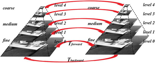
To reduce computational complexity, we proposed a simple two stage bi-direction estimation method. As shown in Figure 3, the first stage in our scheme is to calculate the motion in a single direction which is the same as the conventional pyramid methods. The image pyramid is built with image resolutions being halved at each level. The motion estimation is first executed at top pyramid level with the lowest resolution, then it can be propagated downward as an initialization for the next level. The second stage is that we only propose additional inverse calculation at the last layer assumed $\xi$ with a good initial value. As a result, we can obtain a refined estimate of the motion.

Bi-direction Estimation with Loose Coupling

In addition to the above bi-direction estimation method, another strategy to leverage the motion bias is to run the whole algorithm forward and backward, respectively. Then a refined estimate of the motion can be obtained directly by calculating the average of two results.

Transform Average with Weights

Let ${\mathbf{T}}_f=\left({\mathbf{R}}_1,{\mathbf{t}}_1\right)$ and ${\mathbf{T}}_b^{-1}=\left({\mathbf{R}}_2,{\mathbf{t}}_2\right)$ be the two results of the frame to frame motion estimation. We define weights by photometric errors to describe the contribution of each transform:

(15) ${\omega }_1=\frac{e_2}{e_1+e_2},{\omega }_2=1-{\omega }_1$(15)

where $e_1$ and $e_2$ are the mean photometric errors under transforms ${\mathbf{T}}_f$ and ${\mathbf{T}}_b$. Since the rotation part of the transform is nonlinear and translation part is linear, those two parts should be calculated separately.

First, we use quaternions ${\mathbf{q}}_1$ and ${\mathbf{q}}_2$ to represent rotation matrix ${\mathbf{R}}_1$ and ${\mathbf{R}}_2$. Then the mean quaternion is obtained by the weighted averaging quaternions method proposed in Markley et al.’s paper (Markley et al. 2007):

(16) $\bar{q}=arg\underset{\mathbf{q}\in {\mathbb{S}}^3}{max}{\mathbf{q}}^T\mathbf{M}\mathbf{q}$(16)

where $\mathbf{M}\stackrel{\mathrm{\Delta }}{=}\sum _{i=1}^2{\omega }_i{\mathbf{q}}_i{\mathbf{q}}_i^T$ is a $4\times 4$ matrix.

Second, translation is computed with the linear weighting directly as follows:

(17) $\bar{t}={\omega }_1{\mathbf{t}}_1+{\omega }_2{\mathbf{t}}_2$(17)

Finally, we convert quaternion and translation into the form of transformation matrix to obtain a new estimation.

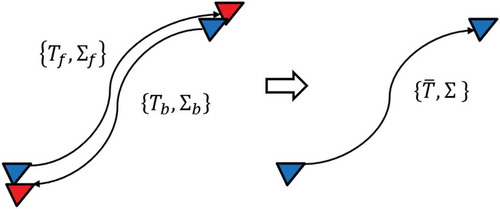
Transform Fusion with Covariance

In addition to using reprojection photometric errors to set weights, we can also use uncertainty to analyze the accuracy of pose estimation. In this section, as depicted in Figure 4, the optimal estimation is fused by two estimations with covariance. We define two $6\times 6$ covariance matrices ${\mathbf{\Sigma }}_f$ and ${\mathbf{\Sigma }}_b$ to express the uncertainty of forward and backward motion transformation (${\xi }_f$ and ${\xi }_b$) respectively.

(18) ${\mathrm{\Sigma }}_f=cov\left({\xi }_f\right)={\left(J_f^T{W}_f{J}_f\right)}^{-1}$(18)

(19) ${\mathrm{\Sigma }}_b=cov\left({\xi }_b\right)={\left(J_b^T{W}_b{J}_b\right)}^{-1}$(19)

where $W_f$ and $W_b$ denote the photometric uncertainty of all measurements described by student’s t-distribution in Equation (8)(8) $w\left(r_i\right)=\frac{\nu +1}{\nu +{\left(\frac{r_i}{\sigma }\right)}^2}$(8) . $J_f$ and $J_b$ are Jacobian matrixs defined in Equation (6)(6) ${\mathbf{J}}_i=\frac{\mathrm{\partial }{r}_i}{\mathrm{\partial }\mathbf{x}}=\frac{\mathrm{\partial }{\mathbf{I}}_c}{\mathrm{\partial }{\mathbf{x}}_i}\frac{\mathrm{\partial }{\mathbf{x}}_i}{\mathrm{\partial }{\mathbf{P}}_i}\frac{\mathrm{\partial }{\mathbf{P}}_i}{\mathrm{\partial }\mathbf{x}}$(6) .

To combine forward and backward estimates conveniently, we calculate optimal motion transformation $\bar{\xi }$ directly in a closed form in $se(3)$.

(20) $\bar{\xi }={\left({\mathrm{\Sigma }}_f^{-1}+{\mathrm{\Sigma }}_b^{-1}\right)}^{-1}\left({\mathrm{\Sigma }}_f^{-1}{\xi }_f-{\mathrm{\Sigma }}_b^{-1}{\xi }_b\right)$(20)

Then the optimal estimation $\bar{T}$ is obtained by $\bar{\xi }$ with the exponential map.

(21) $\bar{T}=\mathbf{T}\left(\bar{\xi }\right)$(21)

Figure 4. Combining forward and backward pose estimates into a single fused estimate with covariance

Evaluation

In this section, we propose a series of experiments on the TUM RGB-D benchmark (Sturm et al. 2012) and ICL-NUIM datasets (Handa et al. 2014). As recommended by Sturm et al. (Sturm et al. 2012), we use the root mean square error (RMSE) of the translational component of relative pose error (RPE) as metric. It is more suitable to measure the drift in frame to frame motion estimation.

(22) $E_i={\left(Q_i^{-1}{Q}_{i+\mathrm{\Delta }t}\right)}^{-1}\left(B_i^{-1}{B}_{i+\mathrm{\Delta }t}\right)$(22)

where $Q_i\in SE(3)$ and $B_i\in SE(3)$ are the ground truth pose and estimated pose of the sequence, respectively.

Due to the measurement error of RGB-D sensor increases with measurement distance increasing, we only select the pixel where depth value greater than 0.5 m and less than 4.5 m. In multi-resolution optimization process, the total level of pyramid is 5 and Gauss-Newton algorithm will run until cost function update less than 0.003 or 20 iterations are reached. The degrees of freedom of the t-distribution $\nu$ is set at 5 as the same in (Kerl, Sturm, and Cremers 2013). GradM is calculated with a Sobel kernel and threshold is 0.0235 for pixel selection. For fast prototyping, we implement all the proposed algorithms in unoptimized MATLAB code. All experiments are carried out on a laptop with Intel i7-7700HQ CPU (2.80 GHz) and 16 GB RAM.

Analysis of Motion Bias

Figure 5. Results on ICL-NUIM assuming no noise (a), ICL-NUIM with simulated noise (b) and TUM RGB-D (e) datasets with different algorithms (c) for each row. Each column of (a) and (c) represents the same sequence which listed in (d). The sequence names of (e) are also listed in (f). The RMSE of the translational RPEs are color coded and shown as small blocks

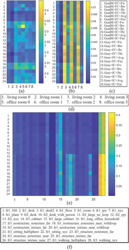
Figure 6. Histogram of the differences between the estimated position and ground truth on x, y, or z axis. Red and blue represent forward and backward respectively

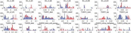
Figure 7. Boxplot of the differences between the estimated position and ground truth on x, y, or z axis. Red and blue represent forward and backward respectively

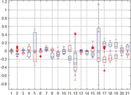
Figure 8. Bi-directional estimation quantity analysis. The estimated trajectories of four methods on the fr2/xyz sequence of TUM dataset is ploted in different solid colors which black, blue, and yellow express x-axis, y-axis, and z-axis respectively. Ground truth is shown as a red dotted line for all axes

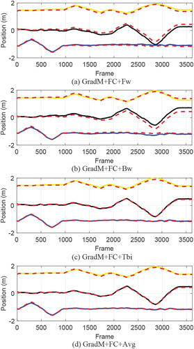
Figure 9. Comparison of reprojection in different directions in the fr2/xyz sequence of TUM dataset. (a) Gray image in Frame 296. (b) Forward reprojection result from Frame 296 to 300. (c) Enlarged detail of gray image in Frame 296. (d) Enlarged detail of forward reprojection result. (e) Gray image in Frame 300. (f) Backward reprojection result from Frame 300 to 296. (g) Enlarged detail of gray image in Frame 300. (h) Enlarged detail of backward reprojection result

To enhance our experiments, we evaluate the performance of all combinations of the following methods: (1) error metric: Intensity (Gray), Gradient magnitude (GradM); (2) alignment strategy: Forward-Compositional (FC), Inverse-Compositional (IC); (3) combined strategy: Forward (Fw), Backward (Bw), Joint bi-direction (Jbi), Two stage bi-direction (Tbi), Transform average with weights (Avg), and Transform fusion with covariance (Fus).

We run the methods on almost all the sequences in the TUM RGB-D and ICL-NUIM datasets (noisy and noise-free). As shown in Figure 5, we use different color blocks to represent the RMSE of the translational RPEs. Surprisingly, we did not find obvious inconsistencies in forward and backward motion while bi-directional consideration does improve accuracy on most sequences. The evaluation indicator is generally positive because it is calculated in square mode. In order to show the positive and negative, we use histogram and boxplot to display the differences between the estimated position and ground truth on x, y, or z axis as shown in Figures 6 and 7. We can clearly see that the statistical means of forward and backward results are on each sides of 0. Different direction calculation will result in different signs of error. So the differences between the RMSE of the translational RPEs are not apparent since the absolute values are close to each other.

Furthermore, we take the sequence fr2/desk as an example and try to explain why add inverse direction calculation can improve accuracy. As shown in Figure 8, the most obvious phenomenon is that the x-axis position is always smaller than the ground truth when calculating forward. Conversely, the x-axis position is generally greater than the ground truth when calculating backward. Since the optimization objective function is not monotonous, calculations in different directions will cause it to converge to different local values. Besides, the range measurements of depth sensor (Kinect) will be affected by factors such as the material of the object, the environment lighting and camera angle. So the difference of missing data at the edges of depth map from different views will also result in forward/backward reprojection images inconsistent (as shown in Figure 9). We can clearly find that the two methods of bi-directional estimation make the results closer to the ground truth and offset the forward and backward differences.

Effect of Composed Methods

Overall, we evaluate 24 possible combinations as shown in Figure 5(c). The results indicate that the GradM-based methods perform better on real-world sequences than synthetic, especially for non-structure environments (fr3_nostructure_notexture_far, fr3_nostructure_notexture_near_withloop, fr3_nostructure_texture_far, and fr3_nostructure_texture_near_withloop, corresponding to the columns 17, 18, 19, and 20 in Figure 5(e)). Meanwhile, the algorithms running on ICL-NUIM dataset show better performance than TUM RGB-D as a whole due to the higher-quality images and simpler environmental conditions.

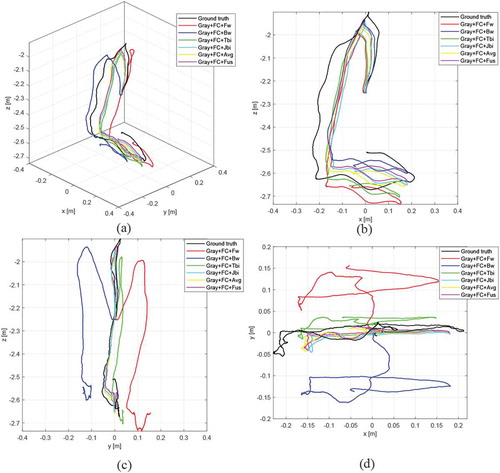
For further illustration, we also provide four sequences, each from ICL-NUIM dataset with simulated noise and TUM RGB-D dataset, for quantitative evaluation as shown in Table 1. We can obviously find that the methods with bi-directional calculation (Jbi, Tbi, Avg, and Fus) significantly improve the accuracy of the odometry. At the same time, we also find that the bi-directional pyramid estimation method (Tbi) has the best results on most sequences. Compared with handling data together (Jbi), Tbi can better utilize the data due to whose additional backward estimation already well initialized with forward estimation. The results of transform fusion with covariance (Fus) are slightly better than the weighted transform average (Avg). As shown in Figure 10, we plot the estimated trajectories of five methods to explain the benefits of bi-directional consideration. The red curve and blue curve clearly show the positive and negative difference on y-axis. After the forward and backward calculations, this part of the error is offset.

Table 1. Results of the RMSE of the translational RPE[m/s]. The “deskp” is short for “desk with person”. The “lr” and “of” also represent living room and office room in ICL-NUIM dataset with simulated noise. The bold indicates the best value and the underline indicates the second best

	lr kt0	lr kt1	of kt0	of kt1	fr1/360	fr2/deskp	fr2/rpy	fr2/xyz	average
Gray+FC+Fw	0.0313	0.0195	0.0629	0.0266	0.0935	0.0185	0.0057	0.0076	0.0332
Gray+IC+Fw	0.0362	0.0212	0.0659	0.0292	0.0861	0.0219	0.0073	0.0095	0.0346
Gray+FC+Bw	0.0282	0.0186	0.0587	0.0278	0.0819	0.0186	0.0057	0.0071	0.0308
Gray+IC+Bw	0.0327	0.0212	0.0631	0.0330	0.0873	0.0220	0.0071	0.0087	0.0344
Gray+FC+Tbi	0.0302	0.0183	0.0613	0.0254	0.0822	0.0150	0.0037	0.0049	0.0301
Gray+IC+Tbi	0.0345	0.0189	0.0647	0.0281	0.0828	0.0172	0.0048	0.0063	0.0322
Gray+FC+Jbi	0.0289	0.0165	0.0575	0.0259	0.0851	0.0181	0.0037	0.0062	0.0302
Gray+IC+Jbi	0.0329	0.0172	0.0598	0.0306	0.0857	0.0217	0.0044	0.0077	0.0325
Gray+FC+Avg	0.0289	0.0163	0.0590	0.0260	0.0860	0.0213	0.0037	0.0060	0.0309
Gray+IC+Avg	0.0325	0.0164	0.0608	0.0294	0.0856	0.0170	0.0041	0.0073	0.0316
Gray+FC+Fus	0.0276	0.0153	0.0565	0.0252	0.0884	0.0180	0.0037	0.0060	0.0301
Gray+IC+Fus	0.0311	0.0171	0.0588	0.0292	0.0881	0.0214	0.0041	0.0073	0.0321
GradM+FC+Fw	0.0345	0.0187	0.0574	0.0301	0.0670	0.0178	0.0051	0.0065	0.0297
GradM+IC+Fw	0.0396	0.0203	0.0618	0.0404	0.0713	0.0235	0.0067	0.0089	0.0341
GradM+FC+Bw	0.0315	0.0175	0.0580	0.0287	0.0620	0.0177	0.0052	0.0068	0.0284
GradM+IC+Bw	0.0354	0.0182	0.0680	0.0362	0.0689	0.0240	0.0066	0.0091	0.0333
GradM+FC+Tbi	0.0341	0.0194	0.0561	0.0283	0.0610	0.0138	0.0032	0.0044	0.0276
GradM+IC+Tbi	0.0385	0.0193	0.0600	0.0380	0.0649	0.0180	0.0042	0.0060	0.0311
GradM+FC+Jbi	0.0327	0.0174	0.0566	0.0289	0.0636	0.0172	0.0034	0.0055	0.0282
GradM+IC+Jbi	0.0367	0.0171	0.0608	0.0353	0.0723	0.0235	0.0042	0.0077	0.0322
GradM+FC+Avg	0.0326	0.0173	0.0573	0.0282	0.0638	0.0170	0.0033	0.0055	0.0282
GradM+IC+Avg	0.0356	0.0159	0.0600	0.0332	0.0694	0.0231	0.0040	0.0075	0.0311
GradM+FC+Fus	0.0323	0.0170	0.0562	0.0278	0.0643	0.0171	0.0033	0.0055	0.0280
GradM+IC+Fus	0.0353	0.0157	0.0595	0.0331	0.0720	0.0233	0.0039	0.0075	0.0313

In addition, results on real-world TUM RGB-D dataset also gain agreement with the previous work (Klose, Heise, and Knoll 2013) in which IC can slightly increase the convergence radius and improve the precision in some sequences (e.g., fr1/360). But results on synthetic ICL-NUIM dataset are mainly weak compared with FC.

In general, bi-directional consideration really works for improving the precision of RGB-D visual odometry. From our experiments, we observe that GradM+FC+Tbi and Gray+FC+Tbi have better performance on realistic datasets. So in practice, we usually recommend these two combinations.

Figure 10. The estimated trajectories of Gray+FC+Fw, Gray+FC+Bw, Gray+FC+Tbi, Gray+FC+Avg, and Gray+FC+Fus on the living room1 sequence of ICL-NUIM dataset with simulated noise

Comparison with State-of-the-art Methods

For the performance comparison with the state-of-the-art, we follow the previous research (Christensen and Hebert 2019), which leverages seven sequences on TUM benchmarks and choice two methods (Gray+FC+Tbi and GradM+FC+Tbi) to compare with the following methods: DVO-SLAM (Kerl, Sturm, and Cremers 2013), Canny-VO (Zhou, Li, and Kneip 2018), Canny-FF (Christensen and Hebert 2019), REVO (Schenk and Fraundorfer 2017b), ORB-SLAM2 (Mur-Artal and Tardós 2017), and RGBDSLAM (Endres et al. 2013). DVO-SLAM is a extended algorithm of combined depth error cost, keyframe and loop closure. Canny-FF is a frame to frame edge-direct visual odometry strategy, which leverages the photometric error. Canny-VO is a 3D–2D edge-direct visual odometry using the geometric error with oriented nearest neighbor fields. REVO represents robust edge-based visual odometry using machine-learned edges. ORB-SLAM2 (RGB-D version, there we only use prue tracking part for fair assessment) is the state-of-the-art feature based SLAM method. RGBDSLAM is also feature based method using ICP and graph optimization.

As shown in Table 2, our algorithms perform competitively and achieve better results on more than half of the dataset. The results of the Canny-FF method on some data sets performs better than the proposed method due to which only considers the photometric errors on the edge pixels. Canny-VO also achieves a highly accurate relative pose due to it usage of Canny edge features and nearest neighbor fields which is robust to the change of light. The results of ORB-SLAM2 on fr1/xyz is best due to its good feature matching when scene views does not change much. It is worth noting that our methods are just frame-to-frame motion estimation method without any keyframe or loop closure. We assume that the random noises, missing depth data on edges and other factors, are independent in two frames. Therefore, more information can be excavated by bi-directional estimation. On the other hand, forward motion can also provide a good initial value for backward motion in pyramid optimization so that a refined estimation could be obtained. Compared with DVO-SLAM, an improvement method of (Kerl, Sturm, and Cremers 2013) which is similar to our Gray+FC+Fw, our frame to frame pose estimation algorithm (Gray+FC+Tbi) is still very competitive without any frame-to-keyframe tracking or pose graph optimization techniques. We believe that the proposed method will be better with keyframe technology or local bundle adjustment.

Table 2. Comparison of the performance of our methods with state of the art by the RMSE of the translational RPE [m/s]. The best result is with bold and second is with underscore. For fair comparison, we directly cited the results from the previous research (Zhou, Li, and Kneip 2018) and (Christensen and Hebert 2019)

Seq.	Gray+FC+Tbi	GradM+FC+Tbi	DVO-SLAM	Canny-FF	Canny-VO	REVO	ORB2-SLAM	RGBDSLAM
fr1/xyz	0.02576	0.02677	0.02661	0.02768	0.019	0.03202	0.01470	0.04193
fr1/rpy	0.02581	0.02351	0.04865	0.03126	0.034	0.03553	0.03221	0.07028
fr1/desk	0.03187	0.03643	0.04429	0.03022	0.031	0.07800	0.06178	0.05346
fr1/desk2	0.04901	0.05340	0.05722	0.04387	0.131	0.07056	0.06535	0.06955
fr1/room	0.03962	0.04034	0.06427	0.04830	0.042	0.04816	0.07081	0.06666
fr1/plant	0.02528	0.03155	0.04362	0.02736	0.036	0.03063	0.04218	0.03789
fr2/desk	0.01201	0.01339	0.03248	0.01375	0.008	0.01426	0.03067	0.01400
average	0.02991	0.03220	0.04531	0.03127	0.043	0.04417	0.04539	0.05054

Performance

Figure 11. Comparison of runtime for the eight algorithms on TUM RGB-D datasets

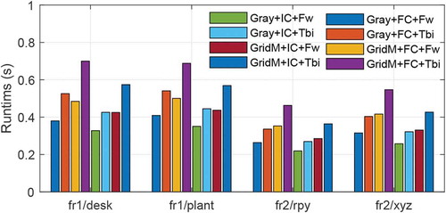
As shown in Figure 11, the average time of the eight algorithms on four datasets are: 0.3421, 0.4515, 0.4386, 0.5994, 0.2888, 0.3655, 0.3696, and 0.4834 (units are seconds). We observe that the GridM-based method does not reduce the time but increases the time. For example, the number of pixels of second frame on fr1/desk dataset in optimization are 232356 and 224233 for gray and GridM method respectively. We use coder profiler (Moore 2017) in MATLAB and find that the overall operating speed is not improved even though the number of points becomes smaller. Extra time comes from the additional gradient calculation. Moreover, pose estimation using IC is really faster than FC. Overall, the bi-directional calculation increases 23.89$\mathrm{\%}$ of single forward estimation. We believe the performance of algorithm will be better when implemented in C/C++, which will be detail discussed in our future research.

Conclusion

In this research, we argue that motion bias plays an important role in the research of direct RGB-D visual odometry through the validation of sufficient experiments. Inspired by the raised completion, a novel bi-directional direct RGB-D visual odometry based on the Bayesian framework is introduced for improving performance using different strategies. For clarifying the contributions of our designed methods, we further investigate the characteristics of proposed methods by extensive experiments. For fair verification, we propose the comparison experiments through a series of popular benchmarks, which further demonstrates the superiorities about the joint optimization using both the forward and backward motions, thus improving motion estimation. In our future research, we intend to embed the designed methods into a complete direct RGB-D SLAM system for further improvements.

Disclosure Statement

No conflict of interest exits in the submission of this manuscript.

Additional information

Funding

This work was supported by the National Natural Science Foundation of China (61773262), and the China Aviation Science Foundation (20142057006).

References

- Aguilar, W. G., G. A. Rodrguez, L. Álvarez, S. Sandoval, F. Quisaguano, and A. Limaico. 2017a. On-board visual SLAM on a UGV using a RGB-D camera. In International Conference on Intelligent Robotics and Applications, 298–308, Springer, Wuhan, China.
- Aguilar, W. G., G. A. Rodrguez, L. Álvarez, S. Sandoval, F. Quisaguano, and A. Limaico. 2017b. Real-time 3D modeling with a RGB-D camera and on-board processing. In International Conference on Augmented Reality, Virtual Reality and Computer Graphics, 410–19, Springer, Ugento, Italy.
- Alismail, H., B. Browning, and S. Lucey. 2016. Enhancing direct camera tracking with dense feature descriptors. In Asian Conference on Computer Vision, 535–51, Springer, Taipei, Taiwan.
- Babu, B. W., S. Kim, Z. Yan, and L. Ren. 2016. σ-dvo: Sensor noise model meets dense visual odometry. In 2016 IEEE International Symposium on Mixed and Augmented Reality (ISMAR), 18–26, IEEE, Merida, Yucatan, Mexico.
- Baker, S., and I. Matthews. 2004. Lucas-kanade 20 years on: A unifying framework. International Journal of Computer Vision 56 (3):221–55. doi:10.1023/B:VISI.0000011205.11775.fd.
- Bergmann, P., R. Wang, and D. Cremers. 2017. Online photometric calibration of auto exposure video for realtime visual odometry and slam. IEEE Robotics and Automation Letters 3 (2):627–34. doi:10.1109/LRA.2017.2777002.
- Christensen, K., and M. Hebert. 2019. Edge-direct visual odometry. arXiv preprint arXiv:1906.04838.
- Civera, J., and S. H. Lee. 2019. RGB-D Image Analysis and Processing. In Advances in Computer Vision and Pattern Recognition, edited by Rosin, P.L., Lai, Y.-K., Shao, L. and Liu, Y., 117-44. Cham: Springer.
- Cvišic, I., J. Cesic, I. Markovic, and I. Petrovic. 2017. Soft-slam: Computationally efficient stereo visual slam for autonomous uavs. Journal of Field Robotics 35 (4):578–595. doi:10.1002/rob.21762.
- Deigmoeller, J., and J. Eggert. 2016. Stereo visual odometry without temporal filtering. In German Conference on Pattern Recognition, 166–75, Springer, Hannover, Germany.
- Dos Reis, D. H., D. Welfer, M. A. De Souza Leite Cuadros, and D. F. T. Gamarra. 2019. Mobile robot navigation using an object recognition software with RGBD images and the YOLO algorithm. Applied Artificial Intelligence 33 (14):1290–305. doi:10.1080/08839514.2019.1684778.
- Endres, F., J. Hess, J. Sturm, D. Cremers, and W. Burgard. 2013. 3-D mapping with an RGB-D camera. IEEE Transactions on Robotics 30 (1):177–87. doi:10.1109/TRO.2013.2279412.
- Engel, J., V. Koltun, and D. Cremers. 2017. Direct sparse odometry. IEEE Transactions on Pattern Analysis and Machine Intelligence 40 (3):611–25. doi:10.1109/TPAMI.2017.2658577.
- Engel, J., V. Usenko, and D. Cremers. 2016. A photometrically calibrated benchmark for monocular visual odometry. arXiv preprint arXiv:1607.02555.
- Handa, A., T. Whelan, J. McDonald, and A. J. Davison. 2014. A benchmark for RGB-D visual odometry, 3D reconstruction and SLAM. In 2014 IEEE international conference on Robotics and automation (ICRA), 1524–31, IEEE, Hong Kong, China.
- Hu, Y., R. Song, and Y. Li. 2016. Efficient coarse-to-fine patchmatch for large displacement optical flow. In Proceedings of the IEEE Conference on Computer Vision and Pattern Recognition, 5704–12, IEEE, Las Vegas, NV, USA.
- Iacono, M., and A. Sgorbissa. 2018. Path following and obstacle avoidance for an autonomous UAV using a depth camera. Robotics and Autonomous Systems 106:38–46. doi:10.1016/j.robot.2018.04.005.
- Kerl, C., J. Sturm, and D. Cremers. 2013. Robust odometry estimation for RGB-D cameras. In 2013 IEEE International Conference on Robotics and Automation, 3748–54, IEEE, Karlsruhe, Germany.
- Klose, S., P. Heise, and A. Knoll. 2013. Efficient compositional approaches for real-time robust direct visual odometry from RGB-D data. In 2013 IEEE/RSJ International Conference on Intelligent Robots and Systems, 1100–06, IEEE, Tokyo, Japan.
- Kuse, M., and S. Shen. 2016. Robust camera motion estimation using direct edge alignment and sub-gradient method. In 2016 IEEE International Conference on Robotics and Automation (ICRA), 573–79, IEEE, Stockholm, Sweden.
- Lin, Y., F. Gao, T. Qin, W. Gao, T. Liu, W. Wu, Z. Yang, and S. Shen. 2018. Autonomous aerial navigation using monocular visual-inertial fusion. Journal of Field Robotics 35 (1):23–51. doi:10.1002/rob.21732.
- Ling, Y., and S. Shen. 2019. Real-time dense mapping for online processing and navigation. Journal of Field Robotics 36 (5):1004–36. doi:10.1002/rob.21868.
- Markley, F. L., Y. Cheng, J. L. Crassidis, and Y. Oshman. 2007. Averaging quaternions. Journal of Guidance, Control, and Dynamics 30 (4):1193–97. doi:10.2514/1.28949.
- Moore, H. 2017. MATLAB for engineers. Upper Saddle River, New Jersey: Pearson.
- Mur-Artal, R., and J. D. Tardós. 2017. Orb-slam2: An open-source slam system for monocular, stereo, and rgb-d cameras. IEEE Transactions on Robotics 33 (5):1255–62. doi:10.1109/TRO.2017.2705103.
- Park, S., T. Schöps, and M. Pollefeys. 2017. Illumination change robustness in direct visual slam. In 2017 IEEE international conference on robotics and automation (ICRA), 4523–30, IEEE, Singapore, Singapore.
- Pereira, F., J. Luft, G. Ilha, A. Sofiatti, and A. Susin. 2017. Backward motion for estimation enhancement in sparse visual odometry. In 2017 Workshop of Computer Vision (WVC), 61–66, IEEE, Natal, Brazil.
- Pillai, S., and J. J. Leonard. 2017. Towards visual ego-motion learning in robots. In 2017 IEEE/RSJ International Conference on Intelligent Robots and Systems (IROS), 5533–40, IEEE, Vancouver, BC, Canada.
- Proesmans, M., L. Van Gool, E. Pauwels, and A. Oosterlinck. 1994. Determination of optical flow and its discontinuities using non-linear diffusion. In European Conference on Computer Vision, 294–304, Springer, Stockholm, Sweden.
- Revaud, J., P. Weinzaepfel, Z. Harchaoui, and C. Schmid. 2015. Epicflow: Edge-preserving interpolation of correspondences for optical flow. In Proceedings of the IEEE conference on computer vision and pattern recognition, 1164–72, IEEE, Boston, MA, USA.
- Schenk, F., and F. Fraundorfer. 2017a. Combining edge images and depth maps for robust visual odometry. In British Machine Vision Conference (BMVC), BMVA Press, London, UK.
- Schenk, F., and F. Fraundorfer. 2017b. Robust edge-based visual odometry using machine-learned edges. In 2017 IEEE/RSJ International Conference on Intelligent Robots and Systems (IROS), 1297–304, IEEE, Vancouver, BC, Canada.
- Schenk, F., and F. Fraundorfer. 2019. RESLAM: A real-time robust edge-based SLAM system. In 2019 International Conference on Robotics and Automation (ICRA), 154–60, IEEE, Montreal, QC, Canada.
- Schops, T., T. Sattler, and M. Pollefeys. 2019. BAD SLAM: Bundle adjusted direct RGB-D SLAM. In Proceedings of the IEEE Conference on Computer Vision and Pattern Recognition, 134–44, IEEE, Long Beach, CA, USA.
- Sturm, J., N. Engelhard, F. Endres, W. Burgard, and D. Cremers. 2012. A benchmark for the evaluation of RGB-D SLAM systems. In 2012 IEEE/RSJ International Conference on Intelligent Robots and Systems, 573–80. IEEE, Vilamoura, Algarve, Portugal.
- Wan, Y., W. Gao, and Y. Wu. 2019. Optical flow assisted monocular visual odometry. In Asian Conference on Pattern Recognition, 366–77, Springer, Auckland, New Zealand.
- Wasenmüller, O., M. D. Ansari, and D. Stricker. 2016. Dna-slam: Dense noise aware slam for tof rgb-d cameras. In Asian Conference on Computer Vision Workshop, 613–29, Springer, Taipei, Taiwan.
- Wong, A., X. Fei, S. Tsuei, and S. Soatto. 2020. Unsupervised depth completion from visual inertial odometry. IEEE Robotics and Automation Letters 5 (2):1899–906. doi:10.1109/LRA.2020.2969938.
- Yang, N., R. Wang, X. Gao, and D. Cremers. 2018. Challenges in monocular visual odometry: Photometric calibration, motion bias, and rolling shutter effect. IEEE Robotics and Automation Letters 3 (4):2878–85. doi:10.1109/LRA.2018.2846813.
- Yin, Z., and J. Shi. 2018. Geonet: Unsupervised learning of dense depth, optical flow and camera pose. In Proceedings of the IEEE Conference on Computer Vision and Pattern Recognition, 1983–92, IEEE, Salt Lake City, UT, USA.
- Zhou, T., P. Krahenbuhl, M. Aubry, Q. Huang, and A. A. Efros. 2016. Learning dense correspondence via 3d-guided cycle consistency. In Proceedings of the IEEE Conference on Computer Vision and Pattern Recognition, 117–26, IEEE, Las Vegas, NV, USA.
- Zhou, Y., H. Li, and L. Kneip. 2018. Canny-vo: Visual odometry with rgb-d cameras based on geometric 3-d–2-d edge alignment. IEEE Transactions on Robotics 35 (1):184–99. doi:10.1109/TRO.2018.2875382.
- Zubizarreta, J., I. Aguinaga, and J. M. M. Montiel. 2020. Direct sparse mapping. IEEE Transactions on Robotics 36 (4):1363–70. doi:10.1109/TRO.2020.2991614.