A Modified Grey Wolf Optimizer Based Data Clustering Algorithm

ABSTRACT

Data clustering is an important data analysis and data mining tool in many fields such as pattern recognition and image processing. The goal of data clustering is to optimally organize similar objects into clusters. Grey wolf optimizer is a newly introduced optimization algorithm with inspiration from the social behavior of gray wolves. In this work, we propose a modified gray wolf optimizer to tackle some of the challenges in meta-heuristic algorithms. These modifications include a balanced approach to the exploration and exploitation stages of the algorithm as well as a local search around the best solution found. The performance of the proposed algorithm is compared to seven other clustering methods on nine data sets from the UCI machine learning laboratory. Experimental results demonstrate the competence of the proposed algorithm in solving data clustering problems. Overall, the intra-cluster distance of the proposed algorithm is lower than other algorithms and gives an average error rate of 11.22% which is the lowest among all.

Introduction

Data clustering which is the practice of organizing a set of objects into groups of objects is one of the most important and common analysis tools for data statistics in many fields of engineering such as machine learning, image processing, signal processing, pattern recognition, and data mining (Jacques and Preda 2014; Mai, Cheng, and Wang 2018; Shirkhorshidi et al. 2014). The goal of clustering is to group data objects into clusters such that the closeness of members belonging to the same group are maximized while closeness of members from different groups is minimized.

Generally, clustering techniques can be divided into two categories of hierarchical clustering and partitional clustering (Celebi 2014; Murtagh and Contreras 2012; Nanda and Panda 2014). One method of hierarchical clustering is to start with assigning each data member to individual clusters and combining more similar clusters into a larger cluster at each step and the other method is to start with the total set of data as one big cluster and breaking it down into smaller clusters until no further improvement is feasible. Partitional clustering, which is the technique utilized in this paper, attempts to divide a set of data objects into a set of non-overlapping clusters without the nested structure. The center of a cluster is called centroid and each data object is initially assigned to the closest centroid and then centroids are updated based on current assignment and by optimizing some criterion (Reynolds et al. 2006).

One of the most popular and widely used partitional clustering algorithms is k-means algorithm which is a fast and simple algorithm that minimizes the average squared distance (Hartigan and Wong 1979). However, k-means efficiency is not only reliant on the initial values of cluster centers but it is also vulnerable to local optimum convergence. Later, k-means++ was proposed to address the sensitivity issue of the standard algorithm to the initial centers (Arthur and Vassilvitskii 2007). However, it failed to solve the problem of convergence to a local optimum (Jain, Murty, and Flynn 1999). In order to overcome this convergence issue and reducing the risk of getting trapped in local optima, we use a meta-heuristic approach to solve the data clustering problem.

In the last few decades, meta-heuristic algorithms have been commonly used to solve NP-hard problems and data clustering falls into the category of NP-hard problems. Several meta-heuristic algorithms have been developed, such as Particle Swarm Optimization (PSO) (Kennedy 2011), Firefly Algorithm (FA) (Yang 2009), Artificial Bee Colony (ABC) algorithm (Karaboga and Basturk 2007), Gravitational Search Algorithm (GSA) (Rashedi, Nezamabadi-pour, and Saryazdi 2009), Simulated Annealing (SA) (Van Laarhoven and Aarts 1987), and Ant Colony Optimization (ACO) (Dorigo and Birattari 2011). A tabu search based method to avoid convergence to local optima in clustering problem was developed which improved k-means by using a tabu search strategy (Lu et al. 2018). Shelokar, Jayaraman, and Kulkarni in 2004 used ACO which mimics the way real ants find the shortest path from their nest to the food source and back to propose an approach to the clustering problem. Artificial bee colony-based algorithm (Zhang, Ouyang, and Ning 2010), particle swarm optimization-based algorithm (Cura 2012), a hybrid of k-means, Medler-Mead simplex, and PSO (Kao, Zahara, and Kao 2008) and a hybrid of PSO and SA (Niknam et al. 2009) are also among the approaches of solving the clustering problem using meta-heuristic algorithms.

Recently, a meta-heuristic technique named gray wolf optimizer (GWO) (Mirjalili, Mirjalili, and Lewis 2014) is used to solve many problems such as load dispatch problem (Kamboj, Bath, and Dhillon 2016), feature subset selection (Emary et al. 2015), concept-based text mining (Thilagavathy and Sabitha 2017), task allocation (Gupta, Ghrera, and Goyal 2018), transmission network expansion planning (Khandelwal et al. 2018), and image segmentation (Mostafa et al. 2016). The promising results of the mentioned literature motivated the authors of this paper to apply a modified version of the GWO algorithm to the data clustering problem.

The remainder of this paper is organized as follows. A summary of data clustering is described in Section “Data Clustering.” Introduction of GWO and the proposed improvements are described in Section “Methodology.” Experimental results on benchmark problems are provided in Section “Experimental Results.” Conclusion of the work is discussed in Section “Conclusion.”

Data Clustering

Extracting information from extensive amounts of data is the main objective of data mining methods. These methods identify compelling patterns in large data sets using data analysis methods. Data analysis methods include clustering, classification, anomaly detection, deviation detection, summarization, and regression. Data clustering is the process of organizing a set of data into subsets such that members of each subset have a high intensity of resemblance while having low resemblance to data in other subsets. The similarity between members of a subset is measured by distance metrics such as Euclidean distance, Chord distance, and Jaccard index. Generally speaking, based on how data is managed and how clusters are formed, clustering methods fall into two main categories: hierarchical and partitional.

In hierarchical clustering, without any advance knowledge of the number of clusters or dependency on the initial condition, a tree which represents a series of clusters is formed (Leung, Zhang, and Xu 2000). However, they are static and an object that belongs to a cluster cannot be assigned to other clusters. This is the primary weakness of hierarchical algorithms. Also, the lack of foresight about the number of clusters may lead to ineffective grouping of overlapping clusters (Jain, Murty, and Flynn 1999). Conversely, partitional clustering separates objects into clusters with a predefined number of clusters. Many partitional clustering algorithms attempt to decrease the dissimilarity between objects within each cluster while increasing the dissimilarity of members assigned to different clusters (Frigui and Krishnapuram 1999).

Problem Formulation

To mathematically formulate the data clustering problem, a set of $N$objects is represented by $X=\left\{X_1,X_2,\dots ,X_N\right\}$. Then, $X_i=\left\{X_i^1,X_i^2,\dots ,X_i^N\right\}$ is a vector representing the $i^{th}$ data object and $x_i^j$ is representing the $j^{th}$ attribute of $x_i$. The objective of clustering is to assign each object in $X$to one of $K$clusters, $C_1$, $C_2$, $\dots$, $C_k$, such that all clusters contain at least one object$(C_i\ne \mathrm{\varnothing };i=1,\dots ,k)$, no object is assigned to more than one cluster $(C_i\cap C_j=\mathrm{\varnothing };i\ne j)$ and all objects are assigned to a cluster $({\cup }_{i=1}^k{C}_i=X)$ (Zhang, Ouyang, and Ning 2010) while minimizing the objective function.

Methodology

Grey wolf optimizer and modifications made to improve its efficiency are presented in this section.

Grey Wolf Optimizer

By taking inspiration from the natural behavior of gray wolves while hunting for prey, a new optimization algorithm called Grey Wolf Optimizer was introduced (Mirjalili, Mirjalili, and Lewis 2014). In this section, the mathematical models for the four stages of this algorithm called surrounding, hunting, searching, and attacking are introduced.

All gray wolves fall into four categories: alpha ($\alpha$), beta ($\beta$), delta ($\delta$), and omega ($\omega$). Alpha wolves which are the decision-makers represent the best solution. The second best solution is represented by beta wolves which provide assistance to alpha wolves. The third best solution is represented by delta wolves, and the remaining solutions are omegas.

The hunting step in GWO is carried out by alpha, beta, and delta wolves while the omega wolves follow their lead. However, before starting to hunt, gray wolves surround the prey. The surrounding operation is modeled by the following equations:

(1) $\vec{D}=|\vec{C}.{\vec{X}}_p-\vec{X}(t)|$(1)

(2) $\vec{X}(t+1)={\vec{X}}_p(t)-\vec{A}.\vec{D}$(2)

where $t$ marks the current iteration, $\vec{A}$ and $\vec{C}$ are coefficient, ${\vec{X}}_p$ represents the position of the prey, and $\vec{X}$ represents the position of a gray wolf.

$\vec{A}$ and $\vec{C}$ are worked out by:

(3) $\vec{A}=2\vec{a}.{\vec{r}}_1-\vec{a}$(3)

(4) $\vec{C}=2{\vec{r}}_2$(4)

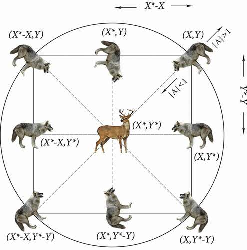
where $\alpha$ is lowered from 2 to 0 over the course of time in a linear manner. Random vectors ${\vec{r}}_1$ and ${\vec{r}}_2$ are in the range of [0, 1]. Using Eq. (1)(1) $\vec{D}=|\vec{C}.{\vec{X}}_p-\vec{X}(t)|$(1) and Eq. (2(2) $\vec{X}(t+1)={\vec{X}}_p(t)-\vec{A}.\vec{D}$(2) ), a gray wolf can move to a new random location in the area around the prey. Figure 1 shows multiple possible positions for a gray wolf based on the position of prey. Coordinates of a gray wolf and the prey are, respectively, $(X,Y)$ and $(X^{\ast },Y^{\ast })$ and different values of $\vec{A}$ and $\vec{C}$ affect the movement direction of a gray wolf.

Figure 1. Possible next positions of a gray wolf

Grey wolves approximate the position of the prey. After all, the position of the prey is unknown, but we can expect that the alpha, beta, and delta wolves to be the nearest to the prey among all wolves. Hence, the position of other wolves is calculated based on the best solutions found so far using the following equations which models the hunting operation:

(5) ${\vec{D}}_{\alpha }=|{\vec{C}}_1.{\vec{X}}_{\alpha }-\vec{X}|$(5)

(6) ${\vec{D}}_{\beta }=|{\vec{C}}_2.{\vec{X}}_{\beta }-\vec{X}|$(6)

(7) ${\vec{D}}_{\delta }=|{\vec{C}}_3.{\vec{X}}_{\delta }-\vec{X}|$(7)

(8) ${\vec{X}}_1={\vec{X}}_{\alpha }-{\vec{A}}_1.({\vec{D}}_{\alpha })$(8)

(9) ${\vec{X}}_2={\vec{X}}_{\beta }-{\vec{A}}_2.({\vec{D}}_{\beta })$(9)

(10) ${\vec{X}}_3={\vec{X}}_{\delta }-{\vec{A}}_3.({\vec{D}}_{\delta })$(10)

(11) $\vec{X}(t+1)=\frac{{\vec{X}}_1+{\vec{X}}_2+{\vec{X}}_3}{3}$(11)

Eqs. (5)(5) ${\vec{D}}_{\alpha }=|{\vec{C}}_1.{\vec{X}}_{\alpha }-\vec{X}|$(5) -(7(7) ${\vec{D}}_{\delta }=|{\vec{C}}_3.{\vec{X}}_{\delta }-\vec{X}|$(7) ) calculate the distance between the prey and alpha, beta, and delta wolves. Eqs. (8)(8) ${\vec{X}}_1={\vec{X}}_{\alpha }-{\vec{A}}_1.({\vec{D}}_{\alpha })$(8) -(10(10) ${\vec{X}}_3={\vec{X}}_{\delta }-{\vec{A}}_3.({\vec{D}}_{\delta })$(10) ) calculate the new position of alpha, beta, and delta wolves while Eq. (11)(11) $\vec{X}(t+1)=\frac{{\vec{X}}_1+{\vec{X}}_2+{\vec{X}}_3}{3}$(11) calculates the position of the prey.

The exploration of search space or searching for prey is accomplished when $|\vec{A}|>1$ which commands the gray wolves to move away from the prey. The coefficient $\vec{C}$ also assists in the searching step. The value of $\vec{C}$ is randomly chosen between 0 and 2 which increases or decreases the impact of prey on distance calculation.

The exploitation of search space or attacking the prey is accomplished when $\vec{A}$ is in the range of −1 and 1. With $|\vec{A}|<1$ the new position of a gray wolf is in any place within its current position and the position of prey, which forces gray wolves to move toward the prey.

Figure 2 depicts the flowchart of gray wolf optimizer. It begins by generating a set of random solutions as the initial population. Best, second best, and third best solutions are chosen as alpha, beta, and delta wolves and the position of each remaining wolf is calculated based on the approximated position of the prey. In conclusion, alpha is returned as the ultimate solution.

Figure 2. Flowchart of gray wolf optimizer

Modified Grey Wolf Optimizer (MGWO)

Exploration and exploitation are two common stages in most optimization algorithms. Exploration is the process of probing the search space. First iterations of an algorithm scan the search space with the hope of finding more fitting solutions. This process allows searching agents to avoid local optima while scanning throughout the search space. Gradually, exploration declines and exploitation rises, so the algorithm can converge to an optimum solution which is the exploitation stage of an algorithm. Finding a proper balance between these two stages is critical to the performance of the algorithm. Hence, proposing a new approach is desirable.

In GWO these two stages are controlled using the parameter $\vec{a}$. As mentioned in the previous section, this parameter is decreased linearly. In earlier iterations of the algorithm, there is more emphasis on exploration and in the later iterations of the algorithm, exploitation is carried out. By changing the linear behavior of $\vec{a}$ we can change the power of exploration and exploitation and come up with a balanced approach between these two stages. Our new control parameter is as followed:

(12) $\vec{a}(t)=2-2{\left(\frac{t}{t_{max}}\right)}^k$(12)

where $t$ indicates the current iteration, $t_{max}$ is the total number of iterations, and $k$ is a constant. Here the parameter $\vec{a}$ is still decreased from 2 to 0 but in a non-linear manner. For the values of $k$ between 0 and 1, the emphasis will be on exploitation; however, the quality of searching capability might suffer. For values of more than 1, search space will be thoroughly explored and then the algorithm moves on to exploitation. A suitable value for $k$should be found by trial and error.

We expect to improve the performance of GWO by the non-linear reduction of the control parameter; however, there is still room for further improvement. In order to make up for the decreased number of iterations that exploit the search space, we use a mapping method to carry out a local search around the best solution. This method maps the best gray wolf position to a new position and if it results in better fitness, the gray wolf will be moved to that place. The new position is calculated as:

(13) ${\vec{X}}_n={\vec{X}}_{\alpha }+r(U-L)(z-0.5)$(13)

where $U$ and $L$are the upper and lower boundaries, $r$ is the center, and $z$ is the mapping parameter which gets updated at each iteration:

(14) ${\vec{z}}_{t+1}=4\times {\vec{z}}_t\times (1-{\vec{z}}_t)$(14)

The modified GWO is expressed by the following pseudo-code.

Algorithm 1. MGWO

Random generation of gray wolves: $X_i(i=1,2,\dots ,n)$

Setting initial values of $\overrightarrow{a}$, $\overrightarrow{A}$, and $\overrightarrow{C}$

$t_{max}$ = total number of iterations

Fitness evaluation of each gray wolf

${\vec{X}}_{\alpha }$: the best solution

${\vec{X}}_{\beta }$: second best solution

${\vec{X}}_{\delta }$: third best solution

while $t<t_{max}$ do

for each ${\vec{X}}_i$ in $\vec{X}$ do

Update the position of ${\vec{X}}_i$

end for

Update $\overrightarrow{a}$, $\overrightarrow{A}$, and $\overrightarrow{C}$

Evaluate the fitness of all gray wolves

Map a new position for ${\vec{X}}_{\alpha }$ and move it there if it’s improved

Update ${\vec{X}}_{\alpha }$, ${\vec{X}}_{\beta }$, and ${\vec{X}}_{\delta }$

$t=t+1$

end while

return ${\vec{X}}_{\alpha }$ as the solution

Solution Encoding and Fitness Function for Data Clustering

Solution encoding is a key step in any meta-heuristic algorithm. Each solution (gray wolf) represents all the cluster centers. Initially, these solutions are generated randomly. However, at each iteration of the GWO, the best solutions (alpha, beta, and delta) guide the rest of the gray wolves. Each solution is an array of size $d\times k$, where $k$is the total number of clusters in the data set and $d$ is the total number of attributes for each data object. A population of gray wolves representing the solutions is shown in Figure 3.

Figure 3. Example of solution encoding

We use the sum of the intra-cluster distance as the objective function. To find optimal cluster centers with MGWO, the objective function should be minimized. Achieving a lower sum of intra-cluster distances is desired. Cluster center is defined in Eq. (15)(15) $y_j=\frac{1}{n_j}\sum _{\mathrm{\forall }{x}_p\in C_j}{x}_p$(15) and distances between cluster members are defined in Eq. (16)(16) $\mathrm{D}\mathrm{i}\mathrm{s}\mathrm{t}\mathrm{a}\mathrm{n}\mathrm{c}\mathrm{e}(x_p-y_j)=\sqrt{\sum _{i=1}^a{(x_{pi}-y_{ji})}^2}$(16) .

(15) $y_j=\frac{1}{n_j}\sum _{\mathrm{\forall }{x}_p\in C_j}{x}_p$(15)

(16) $\mathrm{D}\mathrm{i}\mathrm{s}\mathrm{t}\mathrm{a}\mathrm{n}\mathrm{c}\mathrm{e}(x_p-y_j)=\sqrt{\sum _{i=1}^a{(x_{pi}-y_{ji})}^2}$(16)

Here, $y_j$ is the center of cluster$j$, $x_p$ is the $p^{th}$ member of a cluster. The total number of attributes is represented by $a$, $n_j$ is the number of members in cluster $j$ and $C_j$ are the members of cluster $j$.

Experimental Results

In this section, the quality of MGWO performance is evaluated. First, simulations are carried out on unimodal and multimodal benchmark functions where minimization is the goal and then data clustering using MGWO is performed. In both experiments, a comparison with other algorithms is presented.

Performance Evaluation of MGWO Algorithm

MGWO is tested on 23 standard test problems ($F_1$-$F_{23}$) used by many researchers (Mirjalili and Lewis 2016; Mirjalili, Mirjalili, and Lewis 2014; Rashedi, Nezamabadi-pour, and Saryazdi 2009). These functions have different types of modality and complexity as presented in Table 1. D is the dimension of a function, R is the range of a function’s search space, and ${\mathrm{f}}_{\mathrm{m}\mathrm{i}\mathrm{n}}$ is the minimum of a function. To evaluate the competitiveness of MGWO, it is compared to the standard Grey Wolf Optimizer (GWO) (Mirjalili, Mirjalili, and Lewis 2014), Particle Swarm Optimization (PSO) (Kennedy 2011), Gravitational Search algorithm (GSA) (Rashedi, Nezamabadi-pour, and Saryazdi 2009), and Whale Optimization Algorithm (WOA) (Mirjalili and Lewis 2016). The objective in these test functions is minimization.

Table 1. Definition of standard test functions

Function	D	R	${\mathrm{f}}_{\mathrm{m}\mathrm{i}\mathrm{n}}$
$f_1(x)=\sum _{i=1}^n{x}_i^2$	30	[−100,100]	0
$f_2(x)=\sum _{i=1}^n|x_i|+\prod _{i=1}^n|x_i|$	30	[−10,10]	0
$f_3(x)=\sum _{i=1}^n{(\sum _{j-1}^i{x}_j)}^2$	30	[−100,100]	0
$f_4(x)=ma{x}_i\{|x_i|,1\le i\le n\}$	30	[−100,100]	0
$f_5(x)=\sum _{i=n}^{n-1}\left[100{\left(x_{i+1}-x_i^2\right)}^2+{\left(x_i-1\right)}^2\right]$	30	[−30,30]	0
$f_6(x)=\sum _{i=1}^n{([x_i+0.5])}^2$	30	[−100,100]	0
$f_7(x)=\sum _{i=1}^{n}i{x}_i^4+random[0,1)$	30	[−1.28,1.28]	0
$f_8(x)=\sum _{i=1}^n-x_{i}sin(\sqrt{|x_i|})$	30	[−500,500]	−418.9829 × 5
$f_9(x)=\sum _{i=1}^n\left[x_i^2-10cos\left(2\pi x_i\right)+10\right]$	30	[−5.12,5.12]	0
$f_{10}(x)=-20exp(-0.2\sqrt{\frac{1}{n}\sum _{i=1}^n{x}_i^2})-exp(\frac{1}{n}\sum _{i=1}^{n}cos(2\pi x_i))+20+e$	30	[−32,32]	0
$f_{11}(x)=\frac{1}{4000}\sum _{i=1}^n{x}_i^2-\prod _{i=1}^{n}cos(\frac{x_i}{\sqrt{i}})+1$	30	[−600,600]	0
$\begin{array}{rl}& f_{12}(x)=\frac{\pi }{n}\{10sin(\pi y_i)+\sum _{i=1}^{n-1}{(y_i-1)}^2[1+10{sin}^2(\pi y_{i+1})]+(y_n-1{)}^2\}\\ & +\sum _{i=1}^{n}u(x_i,10,100,4)\\ & y_i=1+\frac{x_i+1}{4}\\ & u(x_i,a,k,m)=\left\{\begin{array}{cc}k{(x_i-a)}^m& x_i>a\\ 0& -a<x_i<a\\ k{(-x_i-a)}^m& x_i<-a\end{array}\right.\end{array}$	30	[−50,50]	0
$\begin{array}{rl}& f_{13}(x)=0.1\{si{n}^2(3\pi x_1)+\sum _{i=1}^n{(x_i-1)}^2[1+si{n}^2(3\pi x_i+1)]\\ & +(x_n-1{)}^2[1+si{n}^2(2\pi x_n)]\}+\sum _{i=1}^{n}u(x_i,5,100,4)\end{array}$	30	[−50,50]	0
$f_{14}(x)=(\frac{1}{500}+\sum _{j=1}^{25}\frac{1}{j+\sum _{i=1}^2{(x_i-a_{ij})}^6}{)}^{-1}$	2	[−65,65]	1
$f_{15}(x)=\sum _{i=1}^{11}{[a_i-\frac{x_i(b_i^2+b_i{x}_2)}{b_i^2+b_i{x}_3+x_4}]}^2$	4	[−5,5]	0.00030
$f_{16}(x)=4x_1^2-2.1x_1^4+\frac{1}{3}{x}_1^6+x_1{x}_2-4x_2^2+4x_2^4$	2	[−5,5]	−1.0316
$f_{17}(x)=(x_2-\frac{5.1}{4{\pi }^2}{x}_1^2+\frac{5}{\pi }{x}_1-6{)}^2+10(1-\frac{1}{8\pi })cos{x}_i+10$	2	[−5,5]	0.398
$\begin{array}{rl}& f_{18}(x)=[1+(x_1+x_2+1{)}^2(19-14x_1+3x_1^2-14x_2+6x_1{x}_2+3x_2^2)]\\ & \times [30+(2x_1-3x_2{)}^2\times (18-32x_1+12x_1^2+48x_2-36x_1{x}_2+27x_2^2)]\end{array}$	2	[−2,2]	3
$f_{19}(x)=-\sum _{i=1}^4{c}_{i}exp(-\sum _{j=1}^3{a}_{ij}(x_j-{p_{ij}}^2)$	3	[1,3]	−3.86
$f_{20}(x)=-\sum _{i=1}^4{c}_{i}exp(-\sum _{j=1}^6{a}_{ij}(x_j-{p_{ij}}^2)$	6	[0,1]	−3.32
$f_{21}(x)=-\sum _{i=1}^5{[(X-a_i){(X-a_i)}^T+c_i]}^{-1}$	4	[0,10]	−10.1532
$f_{22}(x)=-\sum _{i=1}^7{[(X-a_i){(X-a_i)}^T+c_i]}^{-1}$	4	[0,10]	−10.4028
$f_{23}(x)=-\sum _{i=1}^{10}{[(X-a_i){(X-a_i)}^T+c_i]}^{-1}$	4	[0,10]	−10.5363

The total number of search agents is 30 and the total number of iterations is set to 500. Parameters $z$and $k$are, respectively, set to 0.15 and 2. The stopping criterion is reaching the total number of iterations. Our algorithm is independently run 30 times on each test function, mean, and standard deviation results are reported in Table 2. Results show that the overall MGWO gives better results and is superior to the other methods.

Table 2. Results of test problems $F_1$ to $F_{23}$

	MGWO		GWO		PSO		GSA		WOA
	Mean	Std	Mean	Std	Mean	Std	Mean	Std	Mean	Std
F1	5.7849E-36	1.3675E-35	1.7929E-27	3.1886E-27	0.000136	0000202	2.53E-16	9.67E-17	1.41E-30	4.91E-30
F2	9.4232E-22	7.4645E-22	1.2656E-16	1.7063E-16	0.042144	0.045421	0.055655	0.194074	1.06E-21	2.39E-21
F3	6.4878E-07	2.6693E-06	4.3995E-05	0.00014684	70.12562	22.11924	896.5347	318.9559	5.39E-07	2.93E-06
F4	1.2982E-09	2.0487E-09	6.1031E-07	5.5882E-07	1.086481	0.317039	7.35487	1.741452	0.072581	0.39747
F5	26.8472	0.55809	27.1034	0.77555	96.71832	60.11559	67.54309	62.22534	27.86558	0.763626
F6	0.66062	0.38643	0.6712	0.3577	0.000102	8.28E-05	2.5E-16	1.74E-16	3.116266	0.532429
F7	0.0016112	0.00091939	0.0020548	0.0012676	0.122854	0.044957	0.089441	0.04339	0.001425	0.001149
F8	−5516.8023	1129.774	−5838.6035	815.6955	−4841.29	1152.814	−2821.07	493.0375	−5080.76	695.7968
F9	2.4632E-14	7.4165E-14	3.439	6.9524	46.70423	11.62938	25.96841	7.470068	0	0
F10	2.2797E-14	4.5786E-15	1.0581E-13	1.9453E-14	0.276015	0.50901	0.062087	0.23628	7.4043	9.897572
F11	0.0029237	0.0077608	0.0049926	0.0090249	0.009215	0.007724	27.70154	5.040343	0.000289	0.001586
F12	0.03737	0.018899	0.062244	0.097997	0.006917	0.026301	1.799617	0.95114	0.339676	0.214864
F13	0.45877	0.197	0.66336	0.26329	0.006675	0.008907	8.899084	7.126241	1.889015	0.266088
F14	4.556	4.2063	3.2234	3.3473	3.627168	2.560828	5.859838	3.831299	2.111973	2.498594
F15	0.00043824	0.008082	0.0030304	0.0069151	0.000577	0.000222	0.003673	0.001647	0.000572	0.000324
F16	−1.0316	2.0284E-08	−1.0316	3.0386E-08	−1.03163	6.25E-16	−1.03163	4.88E-16	−1.03163	4.2E-07
F17	0.398	4.9031E-05	0.39789	2.8163E-06	0.397887	0	0.397887	0	0.397914	2.7E-05
F18	3	2.6543E-05	3	3.9183E-05	3	1.33E-15	3	4.17E-15	3	4.22E-15
F19	−3.8648	0.0025351	−3.8615	0.0021957	−3.86278	2.58E-15	−3.86278	2.29E-15	−3.85616	0.002706
F20	−3.2699	0.06636	−3.2693	0.066951	−3.26634	0.060516	−3.31778	0.023081	−2.98105	0.376653
F21	−9.8072	1.2858	−9.1408	2.0555	−6.8651	3.019644	−5.95512	3.737079	−7.04918	3.629551
F22	−10.3963	0.0039211	−10.1788	1.2191	−8.45653	3.087094	−9.68447	2.014088	−8.18178	3.829202
F23	−10.2731	1.3981	−9.9034	1.968	−9.95291	1.782786	−10.5364	2.6E-15	−9.34238	2.414737

Exploitation ability of meta-heuristic algorithms is evaluated by unimodal functions $F_1-F_7$since they only have one global minimum. It can be seen from the results that MGWO is the best performing algorithm for functions$F_1$, $F_2$, $F_4$, and $F_5$ while being the second best performing algorithm for functions $F_3$ and $F_7$ which is an indication of excellent exploitation of MGWO.

To evaluate the exploration capability of algorithms, multimodal functions $F_8-F_{23}$ are selected which unlike unimodal functions include multiple local minima. In all multimodal functions but$F_{14}$, MGWO is the best or the second best performing algorithm. GWO is the best algorithm for function$F_8$, PSO gives the best result for $F_{12}$ and $F_{13}$, GSA outperforms other algorithms for $F_{23}$ and WOA is superior for $F_9$, $F_{11}$, and$F_{14}$. Overall the results of the proposed algorithm indicate efficient exploration and exploitation capabilities.

Data Clustering Using MGWO Algorithm

We used nine benchmark data sets from the UCI databases (Blake 1998) which are commonly used in cluster analysis literature. The chosen data sets have a different number of data objects, number of classes, and number of attributes. Three-quarter of data objects in each data set is chosen randomly for training and the remainder is used for testing. Properties of these data sets are provided in Table 3.

Table 3. Characteristics of UCI data sets

Data set	Data objects	Classes	Attributes
Heart	303	2	35
E. Coli	327	5	7
Horse	364	3	58
Dermatology	366	6	34
Cancer	569	2	30
Balance	625	3	4
Credit	690	2	15
Cancer-Int	699	2	9
Diabetes	768	2	8

Heart data set obtained from the Cleveland Heart Clinic database includes 303 objects with 35 attributes. The individuals are grouped into two classes.

E. Coli data set includes information about Escherichia Coli bacterium. Classes with a low number of instances have been removed from this data set. The remaining data has 327 objects and 5 classes.

Horse data set is used for predicting the health situation of a horse with colic disease. Horses are divided into three groups. This data set includes 364 objects and 58 attributes.

Dermatology data set is based on the examination of skin diseases. This data set consists of 366 objects, 34 attributes, and 6 classes.

Cancer data set obtained from the Wisconsin-Diagnostic database groups breast tumors into two classes of mild and deadly. This data set includes 569 objects and 30 attributes.

Balance data set is formed from psychological tests. Each member is classified into one of the three classes: balanced, tip to the left, and tip to the right. This data set includes 625 objects and 4 attributes.

Credit data set is used for the evaluation of credit card applicants in Australia. Data objects in this data set are classified into 2 groups using 15 attributes.

Cancer-Int data set is similar to the Cancer data set but includes 699 objects and 9 attributes instead.

Diabetes data set is the diagnosis of diabetes for patients. A total of 768 objects with 8 attributes are classified into 2 groups of positive and negative.

The total number of search agents is 30 and the total number of iterations is set to 500. Parameters $z$and $k$are, respectively, set to 0.15 and 2. The stopping criterion is reaching the total number of iterations. Results are compared to GSA (Bahrololoum et al. 2012), k-means (Nanda and Panda 2014), PSO (De Falco, Della Cioppa, and Tarantino 2007), K-PSO (Kao, Zahara, and Kao 2008), K-NM-PSO (Kao, Zahara, and Kao 2008), and Firefly Algorithm (Senthilnath, Omkar, and Mani 2011).

Results obtained from these methods are compared based on the sum of intra-cluster distances as well as the error rate. The error rate is the percentage of misclassified data objects in each data set.

Intra-cluster distances obtained from the eight algorithms are provided in Table 4. The values are the average of the sums of intra-cluster distances over 25 runs.

Table 4. Intra-cluster distances of each algorithm on data sets

Data set	MGWO	GWO	GSA	k-means	PSO	K-PSO	K-NM-PSO	FA
Heart	1683.51	2103.95	4350.15	10284.16	2298.83	2144.42	6693.52	9095.10
E.Coli	28.49	42.64	571.97	675.21	40.37	408.93	566.36	57.78
Horse	15.58	18.19	14.85	19.69	8.42	15.10	70.41	94.37
Dermatology	115.83	702.47	654.98	442.87	1862.78	742.20	555.49	1448.48
Cancer	19.53	118.96	34.89	90.25	169.88	29.62	195.20	126.67
Balance	12893.22	21870.25	131293.30	20137.76	61987.01	10966.71	17153.45	37640.44
Credit	1369.16	2403.58	1398.57	3349.21	5090.77	1973.18	4194.19	4036.46
Cancer-Int	96.72	137.45	260.61	148.82	230.30	272.94	150.33	117.52
Diabetes	134.60	3482.75	6747.03	156.52	3140.59	5148.62	9525.25	5488.42

In Credit, Cancer-Int, and Diabetes data sets which have the highest number of data objects, MGWO outperforms all algorithms while PSO, KPSO, and K-NM-PSO have the worst results. Dermatology data set has the highest number of classes which is six classes. Again, our proposed algorithm gives substantially better result on this data set while PSO and FA have the worst results. The only data sets where MGWO doesn’t outperform other algorithms are Horse and Balance. For the Horse data set, PSO gives the best answer followed by GSA, K-PSO, and our proposed algorithm. For Balance data set, MGWO has the second best answer after K-PSO.

Table 5 shows the mean error rate of each algorithm on each data set over 25 simulation runs. For Heart and E. Coli data sets, MGWO has the lowest error rate among all algorithms and k-means, PSO and K-NM-PSO are the worst performing algorithms. For Horse and Dermatology data sets, the mean error rate of K-NM-PSO is the smallest, although, MGWO obtains lower intra-cluster distances for these data sets. It is worth mentioning that since the data distribution in these data sets is not a normal distribution, intra-cluster distance and error rate are not comparable and a lower error rate does not imply a smaller distance.

Table 5. Mean error rate (%) of each algorithm on data sets

Data set	MGWO	GWO	GSA	k-means	PSO	K-PSO	K-NM-PSO	FA
Heart	9.18	17.98	25.01	37.81	16.82	16.26	38.20	19.46
E. Coli	3.92	12.52	7.15	15.51	38.82	21.71	26.31	8.71
Horse	14.22	15.69	7.22	12.31	24.56	12.91	4.06	16.90
Dermatology	11.39	26.73	34.29	40.47	14.39	27.51	5.13	25.37
Cancer	6.04	11.51	12.72	14.62	13.74	6.37	11.77	29.44
Balance	8.27	9.04	3.38	15.11	11.34	36.87	24.19	2.59
Credit	24.70	21.88	14.66	27.67	18.05	36.16	33.33	24.09
Cancer-Int	18.76	16.95	10.09	26.06	8.41	5.76	25.86	7.92
Diabetes	4.53	12.14	7.59	38.30	12.47	2.62	30.76	31.54
Average	11.22	16.04	13.56	25.31	17.62	18.46	22.17	18.44
Rank	1	3	2	8	4	6	7	5

The mean error rate of MGWO is the lowest for Cancer data set which is slightly better than K-PSO. For Balance and Credit data sets, FA and GSA, respectively, have the lowest error rate and K-PSO has the highest error rate in both data sets. For Cancer-Int and Diabetes data sets, K-PSO is the superior algorithm, although MGWO obtains better intra-distances in these instances.

Although MGWO in some data sets does not provide the lowest error rate, it never obtains the highest error rate and the average error rate of MGWO over all data sets is 11.22% which is the lowest and puts it at rank number 1 followed by GSA, GWO, and PSO. k-means and K-NM-PSO have a significantly higher error rate compared to other algorithms.

Conclusion

In this work, we introduced a modified version of a new meta-heuristic optimization method named gray wolf optimizer. The modification is mainly on the importance of the exploration and exploitation aspects of meta-heuristic algorithms and finding a suitable balance between these two stages. The performance of the proposed algorithm was evaluated on well-known benchmark functions and after establishing its superiority compared to PSO, GSA, GWO, and WOA, it was evaluated in terms of intra-cluster distances and error rate on commonly used data clustering benchmark data sets. The results showed that it is overall the better performing algorithm.

Correction Statement

This article has been republished with minor changes. These changes do not impact the academic content of the article.

References

- Arthur, D., and S. Vassilvitskii. 2007. k-means++: The advantages of careful seeding. In Proceedings of the eighteenth annual ACM-SIAM symposium on Discrete algorithms, New Orleans, Louisiana, 1027–35. January.
- Bahrololoum, A., H. Nezamabadi-pour, H. Bahrololoum, and M. Saeed. 2012. A prototype classifier based on gravitational search algorithm. Applied Soft Computing 12 (2):819–25. doi:https://doi.org/10.1016/j.asoc.2011.10.008.
- Blake, C. 1998. UCI repository of machine learning databases. http://www.ics.uci.edu/~mlearn/MLRepository.html.
- Celebi, M. E. 2014. Partitional clustering algorithms. Switzerland: Springer International Publishing.
- Cura, T. 2012. A particle swarm optimization approach to clustering. Expert Systems with Applications 39 (1):1582–88. doi:https://doi.org/10.1016/j.eswa.2011.07.123.
- De Falco, I., A. Della Cioppa, and E. Tarantino. 2007. Facing classification problems with Particle Swarm Optimization. Applied Soft Computing 7 (3):652–58. doi:https://doi.org/10.1016/j.asoc.2005.09.004.
- Dorigo, M., and M. Birattari. 2011. Ant colony optimization. In Sammut C., Webb G.I. (Eds.), Encyclopedia of machine learning, 36–39. Boston, MA: Springer.
- Emary, E., H. Zawbaa, C. Grosan, and A. Hassenian. 2015. Feature Subset Selection Approach by Gray-Wolf Optimization. Advances In Intelligent Systems And Computing 1–13. doi:https://doi.org/10.1007/978-3-319-13572-4_1.
- Frigui, H., and R. Krishnapuram. 1999. A robust competitive clustering algorithm with applications in computer vision. IEEE Transactions On Pattern Analysis And Machine Intelligence 21 (5):450–65. doi:https://doi.org/10.1109/34.765656.
- Gupta, P., S. Ghrera, and M. Goyal. 2018. QoS Aware Grey Wolf Optimization for Task Allocation in Cloud Infrastructure. Proceedings Of First International Conference On Smart System, Innovations And Computing 875–86. doi:https://doi.org/10.1007/978-981-10-5828-8_82.
- Hartigan, J., and M. Wong. 1979. Algorithm AS 136: A K-Means Clustering Algorithm. Applied Statistics 28 (1):100–08. doi:https://doi.org/10.2307/2346830.
- Jacques, J., and C. Preda. 2014. Functional data clustering: A survey. Advances In Data Analysis And Classification 8 (3):231–55. doi:https://doi.org/10.1007/s11634-013-0158-y.
- Jain, A., M. Murty, and P. Flynn. 1999. Data clustering: A review. ACM Computing Surveys 31 (3):264–323. doi:https://doi.org/10.1145/331499.331504.
- Kamboj, V., S. Bath, and J. Dhillon. 2016. Solution of non-convex economic load dispatch problem using Grey Wolf Optimizer. Neural Computing And Applications 27 (5):1301–16. doi:https://doi.org/10.1007/s00521-015-1934-8.
- Kao, Y., E. Zahara, and I. Kao. 2008. A hybridized approach to data clustering. Expert Systems with Applications 34 (3):1754–62. doi:https://doi.org/10.1016/j.eswa.2007.01.028.
- Karaboga, D., and B. Basturk. 2007. A powerful and efficient algorithm for numerical function optimization: Artificial bee colony (ABC) algorithm. Journal Of Global Optimization 39 (3):459–71. doi:https://doi.org/10.1007/s10898-007-9149-x.
- Kennedy, J. 2011. Particle swarm optimization. In Sammut C, Webb G (Eds.), Encyclopedia of machine learning, 760–66. Boston, MA: Springer.
- Khandelwal, A., A. Bhargava, A. Sharma, and H. Sharma. 2018. Modified Grey Wolf Optimization Algorithm for Transmission Network Expansion Planning Problem. Arabian Journal For Science And Engineering 43 (6):2899–908. doi:https://doi.org/10.1007/s13369-017-2967-3.
- Leung, Y., J. S. Zhang, and Z. B. Xu. 2000. Clustering by scale-space filtering. IEEE Transactions On Pattern Analysis And Machine Intelligence 22 (12):1396–410. doi:https://doi.org/10.1109/34.895974.
- Lu, Y., B. Cao, C. Rego, and F. Glover. 2018. A Tabu search based clustering algorithm and its parallel implementation on Spark. Applied Soft Computing 63:97–109. doi:https://doi.org/10.1016/j.asoc.2017.11.038.
- Mai, X., J. Cheng, and S. Wang. 2018. Research on semi supervised K-means clustering algorithm in data mining. Cluster Computing 1–8. doi:https://doi.org/10.1007/s10586-018-2199-7.
- Mirjalili, S., and A. Lewis. 2016. The Whale Optimization Algorithm. Advances in Engineering Software 95:51–67. doi:https://doi.org/10.1016/j.advengsoft.2016.01.008.
- Mirjalili, S., S. Mirjalili, and A. Lewis. 2014. Grey Wolf Optimizer. Advances in Engineering Software 69:46–61. doi:https://doi.org/10.1016/j.advengsoft.2013.12.007.
- Mostafa, A., A. Fouad, M. Houseni, N. Allam, A. Hassanien, H. Hefny, and I. Aslanishvili. 2016. A Hybrid Grey Wolf Based Segmentation with Statistical Image for CT Liver Images. Advances In Intelligent Systems And Computing 846–55. doi:https://doi.org/10.1007/978-3-319-48308-5_81.
- Murtagh, F., and P. Contreras. 2012. Algorithms for hierarchical clustering: An overview. Wiley Interdisciplinary Reviews: Data Mining And Knowledge Discovery 2 (1):86–97. doi:https://doi.org/10.1002/widm.53.
- Nanda, S., and G. Panda. 2014. A survey on nature inspired metaheuristic algorithms for partitional clustering. Swarm And Evolutionary Computation 16:1–18. doi:https://doi.org/10.1016/j.swevo.2013.11.003.
- Niknam, T., B. Amiri, J. Olamaei, and A. Arefi. 2009. An efficient hybrid evolutionary optimization algorithm based on PSO and SA for clustering. Journal Of Zhejiang University-SCIENCE A 10 (4):512–19. doi:https://doi.org/10.1631/jzus.a0820196.
- Rashedi, E., H. Nezamabadi-pour, and S. Saryazdi. 2009. GSA: A Gravitational Search Algorithm. Information Sciences 179 (13):2232–48. doi:https://doi.org/10.1016/j.ins.2009.03.004.
- Reynolds, A., G. Richards, B. de la Iglesia, and V. Rayward-Smith. 2006. Clustering Rules: A Comparison of Partitioning and Hierarchical Clustering Algorithms. Journal Of Mathematical Modelling And Algorithms 5 (4):475–504. doi:https://doi.org/10.1007/s10852-005-9022-1.
- Senthilnath, J., S. Omkar, and V. Mani. 2011. Clustering using firefly algorithm: Performance study. Swarm And Evolutionary Computation 1 (3):164–71. doi:https://doi.org/10.1016/j.swevo.2011.06.003.
- Shelokar, P., V. Jayaraman, and B. Kulkarni. 2004. An ant colony approach for clustering. Analytica chimica acta 509 (2):187–95. doi:https://doi.org/10.1016/j.aca.2003.12.032.
- Shirkhorshidi, A., S. Aghabozorgi, T. Wah, and T. Herawan. 2014. Big Data Clustering: A Review. Computational Science And Its Applications – ICCSA 2014:707–20. doi:https://doi.org/10.1007/978-3-319-09156-3_49.
- Thilagavathy, R., and R. Sabitha. 2017. Using cloud effectively in concept based text mining using grey wolf self organizing feature map. Cluster Computing. doi:https://doi.org/10.1007/s10586-017-1159-y.
- Van Laarhoven, P. J. M., and E. H. L. Aarts. 1987. Simulated annealing. Simulated Annealing: Theory And Applications 37:7–15. doi:https://doi.org/10.1007/978-94-015-7744-1_2.
- Yang, X. S. 2009. Firefly Algorithms for Multimodal Optimization. Stochastic Algorithms: Foundations And Applications 5792:169–78. doi:https://doi.org/10.1007/978-3-642-04944-6_14.
- Zhang, C., D. Ouyang, and J. Ning. 2010. An artificial bee colony approach for clustering. Expert Systems with Applications 37 (7):4761–67. doi:https://doi.org/10.1016/j.eswa.2009.11.003.