General Learning Equilibrium Optimizer: A New Feature Selection Method for Biological Data Classification

ABSTRACT

Finding relevant information from biological data is a critical issue for the study of disease diagnosis, especially when an enormous number of biological features are involved. Intentionally, the feature selection can be an imperative preprocessing step before the classification stage. Equilibrium optimizer (EO) is a recently established metaheuristic algorithm inspired by the principle of dynamic source and sink models when measuring the equilibrium states. In this research, a new variant of EO called general learning equilibrium optimizer (GLEO) is proposed as a wrapper feature selection method. This approach adopts a general learning strategy to help the particles to evade the local areas and improve the capability of finding promising regions. The proposed GLEO aims to identify a subset of informative biological features among a large number of attributes. The performance of the GLEO algorithm is validated on 16 biological datasets, where nine of them represent high dimensionality with a smaller number of instances. The results obtained show the excellent performance of GLEO in terms of fitness value, accuracy, and feature size in comparison with other metaheuristic algorithms.

Introduction

One of the most common challenges in biological data sets is the existence of a large number of variables, which are often called features. The complexity of biological data is gradually growing due to advances in measuring devices (Li et al. 2020; Yamada et al. 2018). Conventionally, the immense amounts of data not only makes the process of classifying them challenging but also increases the complexity (Mafarja et al. 2019). Besides, biological data contain many irrelevant and redundant features, which may adversely degrade the processing accuracy. To remove the noisy information and define the most significant features, the feature selection (FS) process should be considered as a pre-processing step before employing the classifiers to a dataset (Pashaei and Aydin 2017; Zhang et al. 2015).

There are two types of FS in the literature: filter and wrapper. The filter approaches point out the relevant features independently of the learning model. That is, they rank the attributes using the properties of the data and remove all features that do not perceive an adequate score (Hu et al. 2018; Sayed et al. 2019). The wrapper approaches rank the features using a pre-determined learning model, which can select the feature sub-set with a high evaluation measure (Kashef and Nezamabadi-pour 2015). Although the filter is computationally less expensive, the wrapper FS can often produce better results. In wrapper, the FS is known as NP-hard optimization problem (Lu, Yan, and de Silva 2015; Zhang, Shan, and Wang 2017). Hence, many approaches based on metaheuristic algorithms, such as genetic algorithm (Krömer et al. 2018), ant colony optimization (Aghdam, Ghasem-Aghaee, and Basiri 2009), and particle swarm optimization (Chuang et al. 2008) have proposed to assess the efficient solution.

(Kaur, Saini, and Gupta 2018) proposed a parameter-free bat algorithm to find an optimal set of features when classifying brain tumor MR images. The proposed method selected significant features by minimizing the weighted distance between different groups. (Li Zhang et al. 2018) integrated the chaotic attractiveness movement, simulated annealing, and scattering strategies into the firefly algorithm for FS. In their study, the proposed method can often accelerate the convergence and improve the weak solutions, which overtook other conventional algorithms in classification and regression tasks. (Emary, Zawbaa, and Hassanien 2016) developed a novel binary gray wolf optimization for dimensionality reduction. In this approach, a modified sigmoid function was implemented, and it enabled the wolves to conduct the search around the binary feature space. Moreover, (Sindhu et al. 2017) proposed an advanced sine cosine algorithm to tackle the high-dimensional FS in medical datasets. The proposed method utilized elitism strategy to replace the worst agents with quality agents, which ensured high-quality search. The authors in (Too and Abdullah 2020b) proposed a fast rival genetic algorithm in which the competition concept was integrated to boost the performance of the algorithm in FS tasks. Besides, (Amoozegar and Minaei-Bidgoli 2018) developed a multi-objective particle swarm optimization to rank the importance of features by considering the frequency in the archive set. Furthermore, an improved binary dragonfly algorithm was proposed in (Hammouri et al. 2020) for feature selection problems. The authors modified the five main coefficients to overcome the randomness of the algorithm in the diversification and intensification process. More FS studies can be found in (Banka and Dara 2015; Barani, Mirhosseini, and Nezamabadi-pour 2017; Bhadra and Bandyopadhyay 2015; Too and Abdullah 2020a; Wang et al. 2017).

A new metaheuristic algorithm, named Equilibrium Optimizer (EO), has been developed by Faramarzi et al. in 2020 (Faramarzi et al. 2020). Details about the mathematical model and inspiration of the EO is provided in Section 2. Among the early work, EO has shown its superiority against conventional metaheuristic algorithms in several benchmark function tests. However, the EO algorithm has the limitation of restricting the local optimal. Due to the insufficient results and few engineering applications of the EO when compared to other algorithms, this article introduces a new variant of EO, namely general learning equilibrium optimizer (GLEO), to resolve the problem of feature selection in biological data classification. In GLEO, a general learning strategy is proposed to evolve the capability of EO in discovering promising solutions. Unlike EO, GLEO enables the particle to learn from different candidates in multi-dimensions, which is beneficial in preventing the particles from being trapped in the local optimal. Sixteen biological datasets are collected from Arizona State University (ASU) and UCI repository to investigate the usefulness of proposed GLEO in this work. The performance of GLEO is further compared with other six well-known FS algorithms. The experimental results disclose the ascendancy of GLEO not only in higher processing accuracy but also in smaller feature sizes.

The main contributions are summarized as follows:

• A variant version of standard EO is proposed and named GLEO by using a general learning strategy to improve the capability of the EO in exploring the promising regions and escaping the local optimal.

• The proposed GLEO is validated on 16 biological datasets. GLEO overtook other FS algorithms (EO, BOA, GWO, PSO, SCA, and RF).

• The proposed GLEO proved its efficacy based on the obtained solutions and offered excellent results.

Equilibrium Optimizer

Equilibrium optimizer (EO) is a recently established physics-based metaheuristic algorithm in 2020. The EO is inspired by the concept of dynamic source and sink models in measuring equilibrium states (Faramarzi et al. 2020). Like other metaheuristic algorithms, EO generates an initial population of stochastic solutions to start the optimization process. In EO, an initial population of N particles is computed as follows:

(1) $X_i^d=X_{min}+ran{d}_i^d\left(X_{max}-X_{min}\right),i=1,2,\dots ,N\mathrm{a}\mathrm{n}\mathrm{d}d=1,2,\dots ,D$(1)

where X is the position of the particle, N represents the number of particles, D is the number of dimensions, and rand is a random vector between [0, 1]. The X_max and X_min are the maximum and minimum values for the dimensions. After generating the initial population, the particles are evaluated with a specific fitness function, and the equilibrium candidates were identified.

Equilibrium Pool and Candidates

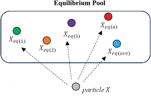
In EO, there is an equilibrium pool to store promising candidates. Correspondingly, four best-so-far particles and their average are stored in the equilibrium pool and will be used for the updating process. These four best-so-far candidates can assist the EO to explore the untried areas, which ensures a high exploration. On the one hand, the average of these candidates can help to exploit the areas near the best solution to find the global optimum. Following this line of thoughts, the equilibrium pool is constructed as follows:

(2) $X_{eq,pool}=\left\{X_{eq\left(1\right)},X_{eq\left(2\right)},X_{eq\left(3\right)},X_{eq\left(4\right)},X_{eq\left(ave\right)}\right\}$(2)

(3) $X_{eq\left(ave\right)}=\frac{X_{eq\left(1\right)}+X_{eq\left(2\right)}+X_{eq\left(3\right)}+X_{eq\left(4\right)}}{4}$(3)

where X_eq,pool is the equilibrium pool, X_eq(1), X_eq(2), X_eq(3), and X_eq(4) are the four best-so-far candidates. The X_eq(ave) is the average of four best-so-far candidates. In each iteration, the particles update their positions with random selection among these five candidates (same probability).

Exponential Term

The exponential term is an important factor that will help EO to maintain a proper balance between global and local searches. The exponential term is defined as follows:

(4) $F=exp\left(-\lambda \left(t-t_0\right)\right)$(4)

where λ is a random vector between [0, 1], t is the time that can be computed as below:

(5) $t={\left(1-\frac{Iter}{MaxIter}\right)}^{\left(\alpha \frac{Iter}{MaxIter}\right)}$(5)

where Iter is the current iteration, MaxIter is the maximum number of iterations, and α is a constant used to control the local search behavior. On the other hand, t₀ is a parameter used to manage exploration and exploitation as follows:

(6) $t_0=\frac{1}{\lambda }In\left(-\beta sign\left(r-0.5\right)\left[1-exp\left(-\lambda t\right)\right]\right)+t$(6)

where r is a random vector between [0, 1], and β is a constant used to manage the exploration capability. As given in Equation (6)(6) $t_0=\frac{1}{\lambda }In\left(-\beta sign\left(r-0.5\right)\left[1-exp\left(-\lambda t\right)\right]\right)+t$(6) , the larger the value of β, the better the exploration capability. According to (Faramarzi et al. 2020), α and β are equal to 1 and 2, respectively. By substituting the Equation (6)(6) $t_0=\frac{1}{\lambda }In\left(-\beta sign\left(r-0.5\right)\left[1-exp\left(-\lambda t\right)\right]\right)+t$(6) into Equation (4)(4) $F=exp\left(-\lambda \left(t-t_0\right)\right)$(4) , the final version of the exponential term can be redefined as below:

(7) $F=\beta sign\left(r-0.5\right)\left[exp\left(-\lambda t\right)-1\right]$(7)

Generation Rate

Another important factor in EO is the generation rate. Intuitively, the generation rate helps the EO to explore the search domain. In EO, the generation rate (G) is formulated as follows:

(8) $G=G_{0}exp\left(-\lambda \left(t-t_0\right)\right)=G_{0}F$(8)

(9) $G_0=GCP\left(X_{eq}-\lambda X\right)$(9)

(10) $GCP=\left\{\begin{array}{c}0.5r_1{r}_2\ge GP\\ 0r_2<GP\end{array}\right.$(10)

where r₁ and r₂ are two random vectors between [0, 1], respectively. The GCP is the generation rate control parameter, and it is computed using Equation (10)(10) $GCP=\left\{\begin{array}{c}0.5r_1{r}_2\ge GP\\ 0r_2<GP\end{array}\right.$(10) . Eventually, the updating rule of EO is defined as:

(11) $X=X_{eq}+\left(X-X_{eq}\right)F+\frac{G}{\lambda V}\left(1-F\right)$(11)

where F is the exponential term, G is the generate rate, X_eq is a random candidate from equilibrium pool, and V is a constant unit with a value equal to 1 (Faramarzi et al. 2020).

Memory Saving

In EO, a mechanism resembles the pbest concept in particle swarm optimization is implemented. If the fitness value attained by the particle in the present iteration is better than the previous iteration, then the particle with better fitness will be saved and stored in pbest. The pseudocode of the EO algorithm is displayed in Algorithm 1.

Table

Algorithm 1. Equilibrium optimizer

1) Initialize a population of N particles using (1)

2) Assign the parameters α = 1; β = 2; GP = 0.5;

3) for (Iter = 1 to MaxIter)

4) for i = 1 to N

5) Evaluate the fitness of Xi

6) Update four best-so-far candidates, Xeq(1), Xeq(2), Xeq(3), Xeq(4)

7) end for

8) Compute Xeq(ave) using (3)

9) Construct the equilibrium pool as shown in (2)

10) Accomplish memory saving

11) Compute t using (5)

12) for i = 1 to N

13) Randomly select one candidate from equilibrium pool

14) Construct F as shown in (7)

15) Compute G using (8)

16) Update the Xi using (11)

17) end for

18) end for

Output: Best candidate, Xeq(1)

General Learning Equilibrium Optimizer

Generally speaking, EO has the benefits and advantages of being casual, adaptable, and flexible, as compared to other metaheuristic optimization algorithms (Faramarzi et al. 2020). However, the performance of EO is still far from perfect. Besides, EO has the limitation of restricting the local optimal. As given in Equation (11)(11) $X=X_{eq}+\left(X-X_{eq}\right)F+\frac{G}{\lambda V}\left(1-F\right)$(11) , the particles are guided by X_eq to move toward the global optimum. Recall that X_eq is a random candidate selected from the equilibrium pool. It means that each particle is learning from a randomly selected candidate in the updating process. The particle might have the difficulty of searching the promising regions if the selected candidate is trapped in the local optimal.

In this article, a new variant of EO, namely general learning equilibrium optimizer (GLEO) is proposed to promote the performance of the EO algorithm. The main idea of general learning is originated from (Liang et al. 2006). The GLEO utilizes a general learning strategy (see Figure 1) that enables the particles to learn from the potential candidates in different dimensions, which can assist the algorithm to escape the local optimal and explore more promising regions.

Figure 1. Basic concept of general learning strategy

General Learning Strategy

In this general learning strategy, the particle is updated as follows:

(12) $X^d=X_{feq\left(d\right)}^d+\left(X^d-X_{feq\left(d\right)}^d\right)F+\frac{G}{\lambda V}\left(1-F\right)$(12)

(13) $G=G_{0}F=\left(GCP\left(X_{feq\left(d\right)}^d-\lambda X^d\right)\right)\cdot F$(13)

where feq = [feq(1), feq(2), …,feq(D)] defines which candidate the particle should follow. The X^d_feq(d) can be the corresponding dth dimension of any candidate in the equilibrium pool. Unlike EO, the candidates of each particle are selected randomly for each dimension. In an alternative word, the particle is learning from different candidates to explore the promising regions.

All the X_feq can generate new positions in the search space using the information offered by different candidates in the equilibrium pool. Therefore, to ensure the particle learns from good candidates and prevents poor direction, the feq will be refreshed only when the fitness value obtained by the current particle is worse than its pbest. With a general learning strategy, it is believed that the search capability and diversity of GLEO can be dramatically enhanced. The pseudocode of GLEO is presented in Algorithm 2.

Table

Algorithm 2. General Learning Equilibrium optimizer

1) Initialize a population of N particles using (1)

2) Assign the parameters α = 1; β = 2; GP = .5;

3) for (Iter = 1 to MaxIter)

4) for i = 1 to N

5) Evaluate the fitness of Xi

6) Update four best-so-far candidates, Xeq(1), Xeq(2), Xeq(3), Xeq(4)

7) end for

8) Compute Xeq(ave) using (3)

9) Construct the equilibrium pool as shown in (2)

10) for i = 1 to N

11) if Xi better than pbesti

12) refreshi = 0

13) else

14) refreshi = 1

15) end if

16) end for

17) Accomplish memory saving

18) Compute t using (5)

19) for i = 1 to N

20) if refreshi = = 1

21) for d = 1 to D

22) Random one candidate from equilibrium pool

23) Store selected index in feq(i, d)

24) end for

25) end if

26) end for

27) for i = 1 to N

28) Construct F as shown in (7)

29) Compute G using (13)

30) Update the Xi using (12)

31) end for

32) end for

Output: Best candidate, Xeq(1)

Proposed GLEO for Feature Selection

Figure 2 illustrates the block diagram of the proposed GLEO for biological data classification. In the first stage, the biological features are collected from the biological dataset to construct the feature set. Due to the high dimensionality of the biological feature set, the Pearson correlation coefficient is used to remove and filter some unwanted features . Then, the GLEO is employed to identify the most informative feature sub-set.

Figure 2. Block diagram of proposed GLEO for biological data classification

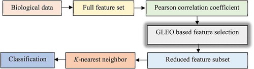
The GLEO starts the FS by creating a set of initial solutions with size (N × D), where N is the number of particles, and D is the number of features. In the population, each vector represents the indices of corresponding features. A threshold of 0.5 is employed to determine whether the feature is selected or not.

(14) $\left\{\begin{array}{c}{x}_i^d>0.5,\mathrm{S}\mathrm{e}\mathrm{l}\mathrm{e}\mathrm{c}\mathrm{t}\mathrm{e}\mathrm{d}\mathrm{f}\mathrm{e}\mathrm{a}\mathrm{t}\mathrm{u}\mathrm{r}\mathrm{e}\\ x_i^d\le 0.5,\mathrm{U}\mathrm{n}\mathrm{s}\mathrm{e}\mathrm{l}\mathrm{e}\mathrm{c}\mathrm{t}\mathrm{e}\mathrm{d}\mathrm{f}\mathrm{e}\mathrm{a}\mathrm{t}\mathrm{u}\mathrm{r}\mathrm{e}\end{array}\right.$(14)

As given in Equation (14)(14) $\left\{\begin{array}{c}{x}_i^d>0.5,\mathrm{S}\mathrm{e}\mathrm{l}\mathrm{e}\mathrm{c}\mathrm{t}\mathrm{e}\mathrm{d}\mathrm{f}\mathrm{e}\mathrm{a}\mathrm{t}\mathrm{u}\mathrm{r}\mathrm{e}\\ x_i^d\le 0.5,\mathrm{U}\mathrm{n}\mathrm{s}\mathrm{e}\mathrm{l}\mathrm{e}\mathrm{c}\mathrm{t}\mathrm{e}\mathrm{d}\mathrm{f}\mathrm{e}\mathrm{a}\mathrm{t}\mathrm{u}\mathrm{r}\mathrm{e}\end{array}\right.$(14) , if the value of the vector is greater than 0.5, then the corresponding feature is selected. Otherwise, the feature is considered an unselected feature. In GLEO, each particle is evaluated by a fitness function. The fitness function is expressed as follows:

(15) $\downarrow \mathrm{F}\mathrm{i}\mathrm{t}\mathrm{n}\mathrm{e}\mathrm{s}\mathrm{s}\mathrm{F}\mathrm{u}\mathrm{n}\mathrm{c}\mathrm{t}\mathrm{i}\mathrm{o}\mathrm{n}=\gamma CE+\left(1-\gamma \right)\frac{\left|R\right|}{\left|F\right|}$(15)

where CE is the classification error, |R| is the length of reduced feature sub-set, |F| is the number of features, and γ is a control parameter. As given in Equation (15)(15) $\downarrow \mathrm{F}\mathrm{i}\mathrm{t}\mathrm{n}\mathrm{e}\mathrm{s}\mathrm{s}\mathrm{F}\mathrm{u}\mathrm{n}\mathrm{c}\mathrm{t}\mathrm{i}\mathrm{o}\mathrm{n}=\gamma CE+\left(1-\gamma \right)\frac{\left|R\right|}{\left|F\right|}$(15) , the first term measures the prediction power, whereas the second term estimates the ratio of feature size. Iteratively, the proposed GLEO will evolve the initial solutions to find the global best solution (Optimal feature subset), as shown in Algorithm 2. Last but not least, the reduced feature sub-set is fed into the k-nearest neighbor (KNN) for the performance validation process.

Results and Discussions

Biological Data and Performance Metrics

Sixteen biological datasets are collected from ASU and UCI repository to evaluate the effectiveness of proposed GLEO algorithm. Table 1 depicts the detailed of 16 utilized biological datasets. As can be seen, the datasets were made up of various numbers of instances, features, and classes, which can examine the efficacy of the proposed GLEO in different perspectives. From Table 1, one can see that nine datasets consisted of very high dimensions (number of features >1000). The dataset with a larger number of features is more complex and represents a real challenge.

Table 1. Detail of 16 utilized biological datasets

	Name of dataset	Training Samples	Features	Classes	Dimension
1	TOX_171	171	5748	4	High
2	Leukemia	72	7070	2	High
3	Lung_discrete	73	325	7	Medium
4	Lymphoma	96	4026	9	High
5	Colon	62	2000	2	High
6	GLIOMA	50	4434	4	High
7	Prostate_GE	102	5966	2	High
8	CLL_SUB_111	111	11340	3	High
9	nci9	60	9712	9	High
10	Lung	203	3312	5	High
11	Lung Cancer	32	56	3	Low
12	Arrhythmia	452	279	16	Medium
13	Dermatology	366	34	6	Low
14	SPECT Heart	267	22	2	Low
15	HCC Survival	165	49	2	Low
16	SCADI	70	205	7	Medium

Four different statistical measurements are used to investigate the efficacy of proposed GLEO in biological data FS and classification. These performance metrics are fitness value, accuracy, feature size, and running time (Emary, Zawbaa, and Hassanien 2016; Kashef and Nezamabadi-pour 2015).

Comparison of Proposed GLEO with EO Algorithm

In this section, the performance of the GLEO is evaluated and compared to the EO algorithm. The environment settings of the experiment are population size = 10, maximum number of iterations = 100, and the lower and upper boundaries are set at 0 and 1, respectively (Faris et al. 2018). According to (Aljarah et al., 2018; Faris et al. 2018), the γ is set at 0.99 because the classification accuracy is the most important measurement. Each dataset is assessed using stratified K-fold cross-validation. To evaluate the fitness of each solution, the k-nearest neighbor (KNN) is employed, which is one of the best classifier as also investigated in (Aljarah et al., 2018; Ibrahim et al. 2019). Due to the stochastic of metaheuristic algorithms, for each algorithm, the experiment is running for G times. Lastly, the average results obtained from all the simulations are recorded and reported. The K and G are at 10 and 20, respectively.

Figure 3 demonstrates the convergence curves of the GLEO and EO algorithms. As can be seen, GLEO offered a very high diversity. As compared to EO, GLEO can often converge faster to find the global optimum, thus resulting in an optimal feature subset. The cardinal cause for the improved efficacy of the GLEO is that it enables the particle to learn from potential candidates in different dimensions. Hence, in the case of immature convergence, the GLEO can effectively prevent converging to inferior locations.

Figure 3. Convergence curves of GLEO and EO algorithms

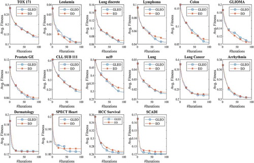
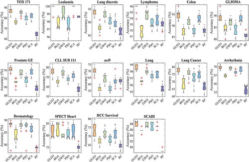
Figure 4. Boxplot of different algorithms

Table 2 presents the results of the GLEO and EO algorithms. From Table 2, GLEO yielded the best fitness value in most cases. Besides, GLEO scored the highest accuracy in at least 14 datasets. Taking dataset 8 (CLL_SUB_111) and dataset 9 (nci9) as the examples, GLEO achieved the optimal accuracies of 76.27% and 70.50%, which proves its superiority in solving the high-dimensional FS problem. Owing to the general learning strategy, GLEO can be capable to avoid local optimal and can effectively get the best solution in this work.

Table 2. Experimental results of GLEO and EO algorithms

No.	Dataset	Performance metrics
		Avg. fitness value		Avg. accuracy		Avg. feature size		Avg. running time (s)
		GLEO	EO	GLEO	EO	GLEO	EO	GLEO	EO
1	TOX_171	0.1338	0.1389	0.8674	0.8621	701.60	679.60	9.848	8.239
2	Leukemia	0.0016	0.0022	0.9986	0.9980	74.55	75.70	3.286	2.138
3	Lung_discrete	0.0638	0.0695	0.9382	0.9325	41.85	43.50	1.100	1.069
4	Lymphoma	0.0431	0.0480	0.9573	0.9526	168.50	212.45	3.088	2.563
5	Colon	0.0550	0.0626	0.9454	0.9376	88.00	79.45	1.718	1.331
6	GLIOMA	0.1063	0.1044	0.8930	0.8950	92.95	89.85	2.277	1.501
7	Prostate_GE	0.0577	0.0594	0.9425	0.9407	237.10	206.80	4.009	3.073
8	CLL_SUB_111	0.2368	0.2453	0.7627	0.7541	1103.25	1004.40	11.431	8.478
9	nci9	0.2932	0.3171	0.7050	0.6808	571.30	547.65	5.075	3.018
10	Lung	0.0157	0.0170	0.9855	0.9841	218.45	214.90	5.388	4.476
11	Lung Cancer	0.2193	0.2253	0.7808	0.7750	6.55	7.05	0.761	0.772
12	Arrhythmia	0.3033	0.3035	0.6955	0.6951	26.25	23.00	5.508	5.869
13	Dermatology	0.1260	0.1251	0.8795	0.8803	11.50	11.25	4.046	4.368
14	SPECT Heart	0.1856	0.1872	0.8160	0.8144	3.85	3.80	2.252	2.298
15	HCC Survival	0.2637	0.2670	0.7360	0.7328	5.55	5.85	1.519	1.520
16	SCADI	0.1204	0.1231	0.8793	0.8764	9.40	7.75	0.958	0.907

In terms of feature size, GLEO and EO can often remove a large quantity of irrelevant and redundant features from the original datasets. The results affirm the supremacy of GLEO and EO in feature reduction. As for computation time, it is seen that the processing speed of GLEO and EO algorithms were very closed. Based on the results obtained, it can be inferred that GLEO not only offered great prediction power but also excellent in selecting a smaller number of informative features.

Comparison of Proposed GLEO with Other Well-known Algorithms

In this section, the performance of GLEO is further compared with butterfly optimization algorithm (BOA) (Arora and Singh 2018), grey wolf optimizer (GWO) (Mirjalili, Mirjalili, and Lewis 2014), particle swarm optimization (PSO) (Kennedy 2011), sine cosine algorithm (SCA) (Mirjalili 2016) and ReliefF algorithm (RF) (Kira and Rendell 1992). Table 3 outlines the parameter settings of comparison algorithms.

Table 3. Parameter settings of comparison algorithms

Algorithm	Controlling parameter	Set value
BOA	Number of butterflies	10
	Maximum number of iterations	100
	Modular modality, c	0.01
	Switch probability, p	0.8
GWO	Number of wolves	10
	Maximum number of iterations	100
PSO	Number of particles	10
	Maximum number of iterations	100
	w	1
	c1	2
	c2	2
SCA	Number of solutions	10
	Maximum iterations	100
	Alpha, α	2
RF	Number of nearest neighbors	5

Table 4 depicts the result of the average fitness value. From Table 4, GLEO achieved the best fitness value in most datasets (14 datasets), followed by BOA and GWO (one dataset). In a nutshell, GLEO retained very good convergence behavior compared to BOA, GWO, PSO, and SCA methods.

Table 4. Results of the fitness value

No.	Dataset	Avg. fitness value
		GLEO	BOA	GWO	PSO	SCA
1	TOX_171	0.1338	0.2369	0.1500	0.2012	0.1836
2	Leukemia	0.0016	0.0237	0.0099	0.0303	0.0022
3	Lung_discrete	0.0638	0.1243	0.0712	0.0978	0.1075
4	Lymphoma	0.0431	0.0839	0.0542	0.0722	0.0630
5	Colon	0.0550	0.1285	0.0835	0.1282	0.0685
6	GLIOMA	0.1063	0.1583	0.1270	0.1639	0.1102
7	Prostate_GE	0.0577	0.0909	0.0677	0.0872	0.0620
8	CLL_SUB_111	0.2368	0.3446	0.2579	0.3246	0.2807
9	nci9	0.2932	0.4346	0.3568	0.4346	0.3735
10	Lung	0.0157	0.0368	0.0213	0.0315	0.0243
11	Lung Cancer	0.2193	0.3151	0.2420	0.2769	0.2500
12	Arrhythmia	0.3033	0.3516	0.3074	0.3328	0.3128
13	Dermatology	0.1260	0.1655	0.1250	0.1320	0.1397
14	SPECT Heart	0.1856	0.1776	0.1942	0.1914	0.1842
15	HCC Survival	0.2637	0.3281	0.2865	0.3177	0.2861
16	SCADI	0.1204	0.1445	0.1220	0.1301	0.1265

Table 5 outlines the result of the accuracy. Based on the result obtained, GLEO outperformed other algorithms on around 87.5% of the datasets. The result reveals that GLEO worked very well in defining the informative features, especially on high-dimensional datasets. Figure 4, exhibits the boxplot of the accuracy. As can be observed, GLEO obtained the highest median value in most datasets, which contributed better classification performance than BOA, GWO, PSO, SCA, and RF algorithms. GLEO’s superior performance is due to high ability to escape local solutions and avoid immature convergence with the general learning mechanism.

Table 5. Results of the accuracy

No.	Dataset	Avg. accuracy
		Original	GLEO	BOA	GWO	PSO	SCA	RF
1	TOX_171	0.6448	0.8674	0.7633	0.8512	0.8016	0.8157	0.6413
2	Leukemia	0.8824	0.9986	0.9792	0.9912	0.9740	0.9979	0.9865
3	Lung_discrete	0.8479	0.9382	0.8786	0.9309	0.9055	0.8938	0.8645
4	Lymphoma	0.9169	0.9573	0.9186	0.9468	0.9317	0.9372	0.9296
5	Colon	0.7604	0.9454	0.8725	0.9171	0.8749	0.9313	0.8758
6	GLIOMA	0.8480	0.8930	0.8420	0.8730	0.8390	0.8890	0.8190
7	Prostate_GE	0.8714	0.9425	0.9113	0.9332	0.9166	0.9379	0.8975
8	CLL_SUB_111	0.5247	0.7627	0.6536	0.7420	0.6770	0.7173	0.5725
9	nci9	0.4308	0.7050	0.5625	0.6417	0.5658	0.6233	0.6242
10	Lung	0.9558	0.9855	0.9659	0.9804	0.9728	0.9763	0.9553
11	Lung Cancer	0.5496	0.7808	0.6850	0.7583	0.7246	0.7492	0.6671
12	Arrhythmia	0.5452	0.6955	0.6477	0.6914	0.6682	0.6849	0.5635
13	Dermatology	0.8668	0.8795	0.8383	0.8803	0.8735	0.8643	0.7881
14	SPECT Heart	0.7869	0.8160	0.8275	0.8061	0.8095	0.8174	0.7502
15	HCC Survival	0.6100	0.7360	0.6717	0.7133	0.6834	0.7128	0.6437
16	SCADI	0.7864	0.8793	0.8571	0.8779	0.8721	0.8729	0.7879

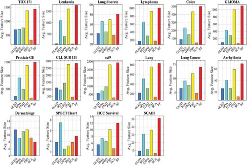
Figure 5 shows the result of the feature size. It is seen that SCA yielded the smallest number of selected features in 13 datasets, followed by GLEO, GWO, and RF (one dataset). Although GLEO is not the best algorithm in feature reduction; however, GLEO can often select the descriptive features that can best describe the target class. Hence, GLEO has attained higher accuracies in this work.

Figure 5. Feature size of different algorithms

Table 6 exhibits the p-values obtained from the Wilcoxon signed-rank test for the pair-wise comparison of the best accuracy achieved from whole iterations with a 5% significance level. Inspecting the result, the performance of GLEO was significantly better than other algorithms in this work. On the whole, GLEO can be inferred as a valuable FS tool in biological data classification.

Table 6. Results of the Wilcoxon test with p-value

No.	Dataset	p-value
		BOA	GWO	PSO	SCA	RF
1	TOX_171	9.00E-05	0.01602	0.00012	0.00029	9.00E-05
2	Leukemia	0.00017	0.00830	8.00E-05	1.00000	0.00013
3	Lung_discrete	9.00E-05	0.09100	0.00019	9.00E-05	9.00E-05
4	Lymphoma	8.00E-05	0.00444	8.00E-05	0.00038	0.00012
5	Colon	9.00E-05	0.00041	9.00E-05	0.04157	9.00E-05
6	GLIOMA	8.00E-05	0.00067	0.00012	0.68335	8.00E-05
7	Prostate_GE	8.00E-05	0.00024	8.00E-05	0.20292	8.00E-05
8	CLL_SUB_111	9.00E-05	0.03994	9.00E-05	0.00034	9.00E-05
9	nci9	8.00E-05	8.00E-05	8.00E-05	8.00E-05	7.00E-05
10	Lung	9.00E-05	0.00447	0.00013	0.00028	9.00E-05
11	Lung Cancer	9.00E-05	0.00689	0.00013	0.00324	8.00E-05
12	Arrhythmia	9.00E-05	0.16704	9.00E-05	0.01054	9.00E-05
13	Dermatology	0.00045	0.04673	0.00327	0.00222	0.00010
14	SPECT Heart	0.20258	0.05273	0.24219	0.78125	9.00E-05
15	HCC Survival	0.00013	0.05521	0.00025	0.04003	9.00E-05
16	SCADI	0.00015	0.75391	0.03674	0.00391	5.00E-05

Conclusion and Future Works

FS is an important pre-processing step before applying the classifier to the datasets. That is, the wrapper-based FS method helps to select the informative features, which is an extremely challenging task in high-dimensional datasets. In this article, a new FS method called GLEO has been developed to solve the FS issue in biological data classification tasks. The integration of general learning strategy within GLEO made it highly capable of searching the promising regions, which can effectively eliminate the redundant and irrelevant information. The experimental results of GLEO implied this algorithm perceived the highest accuracy with the reduced feature sub-set for most of the datasets. The efficacy of GLEO has been proven by verifying the results with EO, BOA, GWO, PSO, SCA, and RF algorithms. Ultimately, GLEO can be considered as a powerful tool in the classification of medical and biological datasets. In the future, GLEO can be hybridized with the other metaheuristic algorithms to further enhance its optimization behavior. Furthermore, the implementation of the general learning strategy as a new mechanism for other metaheuristic algorithms can be investigated in future studies.

Ethical approval

This article does not contain any studies with human participants or animals performed by

any of the authors.

Disclosure statement

No potential conflict of interest was reported by the author(s).

References

- Aghdam, M. H., N. Ghasem-Aghaee, and M. E. Basiri. 2009. Text feature selection using ant colony optimization. Expert Systems with Applications 36 (3,Part 2):6843–53. doi:10.1016/j.eswa.2008.08.022.
- Aljarah, I., M. Mafarja, A. A. Heidari, H. Faris, Y. Zhang, and S. Mirjalili. 2018. Asynchronous accelerating multi-leader salp chains for feature selection. Applied Soft Computing 71:964–79. doi:10.1016/j.asoc.2018.07.040.
- Amoozegar, M., and B. Minaei-Bidgoli. 2018. Optimizing multi-objective PSO based feature selection method using a feature elitism mechanism. Expert Systems with Applications 113:499–514. doi:10.1016/j.eswa.2018.07.013.
- Arora, S., and S. Singh. 2018. Butterfly optimization algorithm: A novel approach for global optimization. Soft Computing. doi:10.1007/s00500-018-3102-4.
- Banka, H., and S. Dara. 2015. A Hamming distance based binary particle swarm optimization (HDBPSO) algorithm for high dimensional feature selection, classification and validation. Pattern Recognition Letters 52 (SupplementC):94–100. doi:10.1016/j.patrec.2014.10.007.
- Barani, F., M. Mirhosseini, and H. Nezamabadi-pour. 2017. Application of binary quantum-inspired gravitational search algorithm in feature subset selection. Applied Intelligence 47 (2):304–18. doi:10.1007/s10489-017-0894-3.
- Bhadra, T., and S. Bandyopadhyay. 2015. Unsupervised feature selection using an improved version of Differential Evolution. Expert Systems with Applications 42 (8):4042–53. doi:10.1016/j.eswa.2014.12.010.
- Chuang, L.-Y., H.-W. Chang, C.-J. Tu, and C.-H. Yang. 2008. Improved binary PSO for feature selection using gene expression data. Computational Biology and Chemistry 32 (1):29–38. doi:10.1016/j.compbiolchem.2007.09.005.
- Emary, E., H. M. Zawbaa, and A. E. Hassanien. 2016. Binary grey wolf optimization approaches for feature selection. Neurocomputing 172:371–81. doi:10.1016/j.neucom.2015.06.083.
- Faramarzi, A., M. Heidarinejad, B. Stephens, and S. Mirjalili. 2020. Equilibrium optimizer: A novel optimization algorithm. Knowledge-Based Systems 191:105190. doi:10.1016/j.knosys.2019.105190.
- Faris, H., M. M. Mafarja, A. A. Heidari, I. Aljarah, A. M. Al-Zoubi, S. Mirjalili, and H. Fujita. 2018. An efficient binary Salp Swarm Algorithm with crossover scheme for feature selection problems. Knowledge-Based Systems 154:43–67. doi:10.1016/j.knosys.2018.05.009.
- Hammouri, A. I., M. Mafarja, M. A. Al-Betar, M. A. Awadallah, and I. Abu-Doush. 2020. An improved Dragonfly Algorithm for feature selection. Knowledge-Based Systems 203:106131. doi:10.1016/j.knosys.2020.106131.
- Hu, L., W. Gao, K. Zhao, P. Zhang, and F. Wang. 2018. Feature selection considering two types of feature relevancy and feature interdependency. Expert Systems with Applications 93:423–34. doi:10.1016/j.eswa.2017.10.016.
- Ibrahim, R. A., A. A. Ewees, D. Oliva, M. Abd Elaziz, and S. Lu. 2019. Improved salp swarm algorithm based on particle swarm optimization for feature selection. Journal of Ambient Intelligence and Humanized Computing 10 (8):3155–69. doi:10.1007/s12652-018-1031-9.
- Kashef, S., and H. Nezamabadi-pour. 2015. An advanced ACO algorithm for feature subset selection. Neurocomputing 147:271–79. doi:10.1016/j.neucom.2014.06.067.
- Kaur, T., B. S. Saini, and S. Gupta. 2018. A novel feature selection method for brain tumor MR image classification based on the Fisher criterion and parameter-free Bat optimization. Neural Computing and Applications 29 (8):193–206. doi:10.1007/s00521-017-2869-z.
- Kennedy, J. 2011. Particle Swarm Optimization. In Encyclopedia of Machine Learning, ed. Claude S., Geoffrey I. W.,760–66. Boston, MA: Springer. doi:10.1007/978-0-387-30164-8_630.
- Kira, K., and L. A. Rendell. 1992. The feature selection problem: Traditional methods and a new algorithm. Proceedings of the Tenth National Conference on Artificial Intelligence, San Jose, California, 129–34.
- Krömer, P., J. Platoš, J. Nowaková, and V. Snášel. 2018. Optimal column subset selection for image classification by genetic algorithms. Annals of Operations Research 265 (2):205–22. doi:10.1007/s10479-016-2331-0.
- Li, C., X. Luo, Y. Qi, Z. Gao, and X. Lin. 2020. A new feature selection algorithm based on relevance, redundancy and complementarity. Computers in Biology and Medicine 119:103667. doi:10.1016/j.compbiomed.2020.103667.
- Liang, J. J., A. K. Qin, P. N. Suganthan, and S. Baskar. 2006. Comprehensive learning particle swarm optimizer for global optimization of multimodal functions. IEEE Transactions on Evolutionary Computation 10 (3):281–95. doi:10.1109/TEVC.2005.857610.
- Lu, L., J. Yan, and C. W. de Silva. 2015. Dominant feature selection for the fault diagnosis of rotary machines using modified genetic algorithm and empirical mode decomposition. Journal of Sound and Vibration 344:464–83. doi:10.1016/j.jsv.2015.01.037.
- Mafarja, M., I. Aljarah, H. Faris, A. I. Hammouri, A. M. Al-Zoubi, and S. Mirjalili. 2019. Binary grasshopper optimisation algorithm approaches for feature selection problems. Expert Systems with Applications 117:267–86. doi:10.1016/j.eswa.2018.09.015.
- Mirjalili, S. 2016. SCA: A Sine Cosine Algorithm for solving optimization problems. Knowledge-Based Systems 96:120–33. doi:10.1016/j.knosys.2015.12.022.
- Mirjalili, S., S. M. Mirjalili, and A. Lewis. 2014. Grey Wolf Optimizer. Advances in Engineering Software 69:46–61. doi:10.1016/j.advengsoft.2013.12.007.
- Pashaei, E., and N. Aydin. 2017. Binary black hole algorithm for feature selection and classification on biological data. Applied Soft Computing 56:94–106. doi:10.1016/j.asoc.2017.03.002.
- Sayed, S., M. Nassef, A. Badr, and I. Farag. 2019. A Nested Genetic Algorithm for feature selection in high-dimensional cancer Microarray datasets. Expert Systems with Applications 121:233–43. doi:10.1016/j.eswa.2018.12.022.
- Sindhu, R., R. Ngadiran, Y. M. Yacob, N. A. H. Zahri, and M. Hariharan. 2017. Sine–cosine algorithm for feature selection with elitism strategy and new updating mechanism. Neural Computing and Applications 28 (10):2947–58. doi:10.1007/s00521-017-2837-7.
- Too, J., and A. R. Abdullah. 2020a. Opposition based competitive grey wolf optimizer for EMG feature selection. Evolutionary Intelligence. doi:10.1007/s12065-020-00441-5.
- Too, J., and A. R. Abdullah. 2020b. A new and fast rival genetic algorithm for feature selection. The Journal of Supercomputing 1–31. doi:10.1007/s11227-020-03378-9.
- Wang, M., Y. Wan, Z. Ye, and X. Lai. 2017. Remote sensing image classification based on the optimal support vector machine and modified binary coded ant colony optimization algorithm. Information Sciences 402:50–68. doi:10.1016/j.ins.2017.03.027.
- Yamada, M., J. Tang, J. Lugo-Martinez, E. Hodzic, R. Shrestha, A. Saha, H. Ouyang, D. Yin, H. Mamitsuka, C. Sahinalp, et al. 2018. Ultra high-dimensional nonlinear feature selection for big biological data. IEEE Transactions on Knowledge and Data Engineering 30 (7):1352–65. doi:10.1109/TKDE.2018.2789451.
- Zhang, L., K. Mistry, C. P. Lim, and S. C. Neoh. 2018. Feature selection using firefly optimization for classification and regression models. Decision Support Systems 106:64–85. doi:10.1016/j.dss.2017.12.001.
- Zhang, L., L. Shan, and J. Wang. 2017. Optimal feature selection using distance-based discrete firefly algorithm with mutual information criterion. Neural Computing and Applications 28 (9):2795–808. doi:10.1007/s00521-016-2204-0.
- Zhang, Y., D. Gong, Y. Hu, and W. Zhang. 2015. Feature selection algorithm based on bare bones particle swarm optimization. Neurocomputing 148:150–57. doi:10.1016/j.neucom.2012.09.049.