Comparative Investigation of Learning Algorithms for Image Classification with Small Dataset

ABSTRACT

Increase in popularity of deep learning in various research areas leads to use it in resolving image classification problems. The objective of this research is to compare and to find learning algorithms which perform better for image classification task with small dataset. We have also tuned the hyperparameters associated with optimizers and models to improve performance. First, we performed several experiments using eight learning algorithms to come closer to optimal values of hyperparameters. Then, we executed twenty-four final experiments with near optimum values of hyperparameters to find the best learning algorithm. Experimental results showed that the AdaGrad learning algorithm achieves better accuracy, lesser training time, as well as fewer memory utilization compared to the rest of the learning algorithms.

Introduction

Machine learning is a subfield of computer science that provides ability to electronic devices to learn automatically and improve their performance without being programmed with any task-specific rules. Arthur Samuel in 1952 made the first learning code game of checkers (Samuel 1959). Deep learning is subclass of machine learning. We typically say it “Deep” when we have more than two layers in network otherwise it is called “Shallow” learning. The study of deep learning started in 1940s (Mcculloch and Pitts 1943) when McCulloch introduce the ideas immanent in nervous activity using calculus. Using massive datasets in deep networks achieved better performance for image recognition (LeCun et al. 1998), video classification (Karpathy et al. 2014), natural language processing (Collobert and Weston 2008), and speech recognition (Hinton et al. 2012) tasks.

There are three main kinds of machine learning: supervised learning, unsupervised learning and reinforcement learning as shown in Figure 1. In supervised learning, we have x as input variables, and try to learn a function mapping from x to y, y is called output variable. For example, we give an image to network as input and want to predict a number from model, say from 0 to 4, it may be any one of a five given images.

Figure 1. Three common forms of machine learning, their subclasses and renowened algorihtms

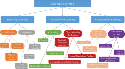
Supervised learning can be further divided into classification and regression. Classification is basically a method of processing some input and mapping it to discrete output. Spam filter is the simplest example of classification; e-mails in inbox are process by machine learning spamming algorithm and if some criteria is fulfilled than e-mails are consider as spam. In regression problem, we try to predict numeric dependences of function value from set of input parameters. For example, housing price prediction and many other engineering problems.

A neural network is a widely used supervised learning algorithm and is inspired by the function of human brain such as learning through experience. Network is automated to learn by examining dataset over and over again, identify and observing underlying relations to construct models, and persistently improving these models.

There are three main types of artificial neural networks: standard neural networks, convolution neural networks and recurrent neural networks. If we want to solve problems such as real estate market prediction and online advertising, we may use the standard neural network. Problems which utilize images as input, convolution neural network is the best choice. Recurrent neural network typically deals with the sequential data problems such as machine translation and speech recognition. For more complex problems such as autonomous driving we may use the combination of these three neural networks.

Convolutional neural network has been studied since 1990s, but it became popular with the following classic networks: LeNet (LeCun et al. 1998), AlexNet (Krizhevsky, Sutskever, and Hinton 2012), VGG (Simonyan and Zisserman 2015), and it has started to be utilized in different research areas such as interpretation of medical images (Iqbal, et al. 2020; Iqbal, Mustafa, and Ma 2020; Iqbal et al. 2021). Deep neural networks are very suitable to solve the problems related to audio, images, speech and video (Lecun, Bengio, and Hinton 2015). There are three types of layer in a convolutional neural network: convolution layer, pooling layer and fully connected layer.

Hyperparameters can be tuned manually or by defined rules. Choosing optimum hyperparameter is as essential as to choose the right learning algorithm such as RMSProp or Adam and choose the correct network architecture such as AlexNet or Inception (Szegedy et al. 2015) in terms of performance of problem.

The objective of this research is to find out the better learning algorithm which can be utilized to train the deep networks for image classification problem with small dataset after tuning the hyperparameters. Several datasets are available for speech recognition task but for image recognition problem there are only a few datasets are available as compared to speech recognition. And lot of GPUs or TPUs resources are needed to train the deep networks using large dataset specially when we tune the hyperparameters.

It has been seen that different learning algorithms are more suitable for different problems. Experiments of this research were performed using Keras and TensorFlow (Abadi et al. 2016) deep programming frameworks. In all experiments eight learning algorithms, which are renowned algorithms, were employed which are SGDNesterov, AdaGrad, RMSProp, AdaDelta, Adam, AdaMax, Nadam and AMSGrad. AdaGrad optimizer achieved best performance on test set when hyperparameters: learning rate (η), mini-batch size (M_b), number of layers (N_l), number of epochs (N_e), tune to near optimum values.

The rest of the article is organized as follows: “Learning algorithms” section briefly describes the detail of eight algorithms which are used in this research work to train the deep networks. “Experiments” section explains the hyperparameters, dataset, and network architectures of this research. “Evaluations” section covers the detailed comparison of accuracy, time, and memory utilization of all algorithms. Finally, the “Conclusions and future work” are discussed in the last section.

Learning Algorithms

In this section, we briefly discuss learning algorithms which we used in this research to train the networks. Gradient descent is a common framework to do optimization task in artificial neural networks. This optimizer can minimize the cost function. Gradient descent parameters are given in Equation (1) and formula for updating parameters is in Equation (2)(2) ${\theta }_{\mathrm{t}+1}={{\theta }_{\mathrm{t}}}_{}-\eta \mathrm{\nabla }\mathrm{L}\left({\theta }_{\mathrm{t}}\right)$(2) .

(1) ${\theta }_{\mathrm{t}}=\left[\begin{array}{c}b\\ w\end{array}\right]$(1)

(2) ${\theta }_{\mathrm{t}+1}={{\theta }_{\mathrm{t}}}_{}-\eta \mathrm{\nabla }\mathrm{L}\left({\theta }_{\mathrm{t}}\right)$(2)

Where b is biases, w is weights, t is a time step, $\theta$ is a parameter, η is a learning rate, $\mathrm{L}\left(\theta \right)$ is a cost function and $\mathrm{\nabla }\mathrm{L}\left(\theta \right)$ is the gradient of cost function.

Stochastic Gradient Descent Algorithm

There are three different types of gradient descent methods: batch gradient descent, mini-batch gradient descent and stochastic gradient descent (SGD) (Robbins and Monro 1951). In batch gradient descent, we calculate the partial derivative of cost function with respect to parameters $\theta$, weights and biases, for the whole training dataset. While in mini-batch gradient descent, we choose mini-batch size and perform an update for each mini-batch. If we choose mini-batch size to one, then it is called SGD. It does not always converge and may be noisy. The update rule of SGD is in Equation (3)(3) ${\theta }_{\mathrm{t}+1}={{\theta }_{\mathrm{t}}}_{}-\eta \mathrm{\nabla }\mathrm{L}\left({\theta }_{\mathrm{t}};{\mathrm{x}}^{\left(\mathrm{i}\right)};{\mathrm{y}}^{\left(\mathrm{i}\right)}\right)$(3) .

(3) ${\theta }_{\mathrm{t}+1}={{\theta }_{\mathrm{t}}}_{}-\eta \mathrm{\nabla }\mathrm{L}\left({\theta }_{\mathrm{t}};{\mathrm{x}}^{\left(\mathrm{i}\right)};{\mathrm{y}}^{\left(\mathrm{i}\right)}\right)$(3)

Where ${\mathrm{x}}^{\left(\mathrm{i}\right)}$is the i^th training example, and ${\mathrm{y}}^{\left(\mathrm{i}\right)}$ is the i^th label.

SGD is a simple and basic algorithm that usually does not give good accuracy. There is a modified version of this method which is called SGD with momentum (Qian 1999) which almost always works better than this simple learning algorithm. Using momentum in SGD, accelerate gradients vectors in the right directions which damp out oscillation and gives us fast convergence. The update equations are Equations (4)(4) ${\mathrm{v}}_{\mathrm{t}}=\beta {\mathrm{v}}_{\mathrm{t}-1}+\eta \hspace{0.17em}\mathrm{\nabla }\mathrm{L}\left({\theta }_{\mathrm{t}}\right)$(4) – (5(5) ${\theta }_{\mathrm{t}+1}={{\theta }_{\mathrm{t}}}_{}-{\mathrm{v}}_{\mathrm{t}}$(5) ).

(4) ${\mathrm{v}}_{\mathrm{t}}=\beta {\mathrm{v}}_{\mathrm{t}-1}+\eta \hspace{0.17em}\mathrm{\nabla }\mathrm{L}\left({\theta }_{\mathrm{t}}\right)$(4)

(5) ${\theta }_{\mathrm{t}+1}={{\theta }_{\mathrm{t}}}_{}-{\mathrm{v}}_{\mathrm{t}}$(5)

Common value for momentum term $\beta$ is from 0.8 to 0.999, where $\mathrm{v}$ is the exponentially weighted moving average.

Nesterov (Nesterov 1983) is another method similar to momentum. Nesterov accelerated gradient (NAG) algorithm calculate the partial derivative with respect to the approximate future position of weights and bias. The equations of this technique are Equations (6)(6) ${\mathrm{v}}_{\mathrm{t}}=\beta {\mathrm{v}}_{\mathrm{t}-1}+\eta \hspace{0.17em}\mathrm{\nabla }\mathrm{L}\left({\theta }_{\mathrm{t}}-\beta {\mathrm{v}}_{\mathrm{t}-1}\right)$(6) – (7(7) ${\theta }_{\mathrm{t}+1}={{\theta }_{\mathrm{t}}}_{}-{\mathrm{v}}_{\mathrm{t}}$(7) ). The default value of η is 0.01.

(6) ${\mathrm{v}}_{\mathrm{t}}=\beta {\mathrm{v}}_{\mathrm{t}-1}+\eta \hspace{0.17em}\mathrm{\nabla }\mathrm{L}\left({\theta }_{\mathrm{t}}-\beta {\mathrm{v}}_{\mathrm{t}-1}\right)$(6)

(7) ${\theta }_{\mathrm{t}+1}={{\theta }_{\mathrm{t}}}_{}-{\mathrm{v}}_{\mathrm{t}}$(7)

Adaptive Gradient Algorithm

Adaptive gradient or AdaGrad (Duchi, Hazan, and Singer 2011) algorithm uses a simple gradient process at each time step, this method takes a different η for every weight and bias. This learning algorithm does slighter change for frequent parameters and greater change for infrequent parameters. The drawback of technique is vanishing η. Parameters update by AdaGrad are given in Equations (8)(8) ${\mathrm{g}}_{\mathrm{t}}=\mathrm{\nabla }\mathrm{L}\left({\theta }_{\mathrm{t}}\right)$(8) – (9(9) ${\theta }_{\mathrm{t}+1}={\theta }_{\mathrm{t}}-\frac{\eta \hspace{0.17em}}{\sqrt{{\mathrm{G}}_{\mathrm{t}}+}}\hspace{0.17em}{\mathrm{g}}_{\mathrm{t}}$(9) ).

(8) ${\mathrm{g}}_{\mathrm{t}}=\mathrm{\nabla }\mathrm{L}\left({\theta }_{\mathrm{t}}\right)$(8)

(9) ${\theta }_{\mathrm{t}+1}={\theta }_{\mathrm{t}}-\frac{\eta \hspace{0.17em}}{\sqrt{{\mathrm{G}}_{\mathrm{t}}+}}\hspace{0.17em}{\mathrm{g}}_{\mathrm{t}}$(9)

Where η is usually set to 0.01, ${\mathrm{G}}_{\mathrm{t}}$ is a diagonal matrix and is an element wise multiplication of matrix and vector. The value of hyperparameter, ε, of this technique does not matter very much because it is just to prevent division by zero, 10⁻⁸ is default value.

Root Mean Square Propagation Algorithm

RMSProp (Hinton, Srivastava, and Swersky 2012), which stands for root mean square prop, this may speed up gradient descent. This technique divides the learning rate η by an exponentially weighted moving averages of squared gradients. This algorithm actually desires to damp out learning in one direction and try to speedup learning in another direction. It was first presented in a Coursera lecture by Geoffrey Hinton. RMSProp usually works well for recurrent neural networks. The update parameters process of this method is given in Equations (10)(10) ${\mathrm{v}}_{\mathrm{t}}=\beta {\mathrm{v}}_{\mathrm{t}-1}+\left(1-\beta \right){\mathrm{g}}_{\mathrm{t}}^2$(10) – (11(11) ${\theta }_{\mathrm{t}+1}={\theta }_{\mathrm{t}}-\hspace{0.17em}\eta \frac{{\mathrm{g}}_{\mathrm{t}}}{\sqrt{{\mathrm{v}}_{\mathrm{t}}+}}$(11) ), where common default value of η in RMSProp is 0.001.

(10) ${\mathrm{v}}_{\mathrm{t}}=\beta {\mathrm{v}}_{\mathrm{t}-1}+\left(1-\beta \right){\mathrm{g}}_{\mathrm{t}}^2$(10)

(11) ${\theta }_{\mathrm{t}+1}={\theta }_{\mathrm{t}}-\hspace{0.17em}\eta \frac{{\mathrm{g}}_{\mathrm{t}}}{\sqrt{{\mathrm{v}}_{\mathrm{t}}+}}$(11)

Adaptive Learning Rate Algorithm

Adaptive learning rate or AdaDelta (Zeiler 2012) optimizer is a modified version of AdaGrad method to resolve the problem of learning rates which frequently vanish. The equations of this learning algorithm are Equations (12)(12) $\mathrm{R}\mathrm{M}\mathrm{S}{\left[\delta \theta \right]}_{\mathrm{t}}=\sqrt{\mathrm{E}{\left[\delta {\theta }^2\right]}_{\mathrm{t}}+}$(12) – (14(14) ${\theta }_{\mathrm{t}+1}={\theta }_{\mathrm{t}}-\delta {\theta }_{\mathrm{t}}$(14) ).

(12) $\mathrm{R}\mathrm{M}\mathrm{S}{\left[\delta \theta \right]}_{\mathrm{t}}=\sqrt{\mathrm{E}{\left[\delta {\theta }^2\right]}_{\mathrm{t}}+}$(12)

(13) ${\delta \theta }_{\mathrm{t}}=\frac{\mathrm{R}\mathrm{M}\mathrm{S}{\left[\theta \right]}_{\mathrm{t}-1}}{\mathrm{R}\mathrm{M}\mathrm{S}{\left[\mathrm{g}\right]}_{\mathrm{t}}}{\mathrm{g}}_{\mathrm{t}}$(13)

(14) ${\theta }_{\mathrm{t}+1}={\theta }_{\mathrm{t}}-\delta {\theta }_{\mathrm{t}}$(14)

Where RMS is parameter root mean squared error, E is a running average.

Adaptive Moment Estimation Algorithm

Adam (Kingma and Ba 2015) stands for adaptive moment estimation; this is most frequently used learning algorithm in neural networks which does not use only the average of the sum of the gradients but also the average of the sum of the squared gradients. This learning algorithm is actually a combination of gradient descent with momentum and gradient descent with RMSProp.

This algorithm has four hyperparameters. The learning rate which is most important and usually set to 0.001. Momentum like term ${\beta }_1$, the default choice is 0.9. The RMSProp like term ${\beta }_2$, the authors of the Adam paper recommend it to 0.999. The choice of last hyperparameter value of ε is 10⁻⁸. The update equations of Adam are shown in Equations (15)(15) ${\mathrm{m}}_{\mathrm{t}}={\beta }_1{\mathrm{m}}_{\mathrm{t}-1}+(1-{\beta }_1){\mathrm{g}}_{\mathrm{t}}$(15) – (19(19) ${\theta }_{\mathrm{t}+1}={\theta }_{\mathrm{t}}-\hspace{0.17em}\frac{{\hat{\mathrm{m}}}_{\mathrm{t}}}{\sqrt{{\hat{\mathrm{v}}}_{\mathrm{t}}}+}$(19) ).

(15) ${\mathrm{m}}_{\mathrm{t}}={\beta }_1{\mathrm{m}}_{\mathrm{t}-1}+(1-{\beta }_1){\mathrm{g}}_{\mathrm{t}}$(15)

(16) ${\mathrm{v}}_{\mathrm{t}}={\beta }_2{\mathrm{v}}_{\mathrm{t}-1}+(1-{\beta }_2){\mathrm{g}}_{\mathrm{t}}^2$(16)

(17) ${\hat{\mathrm{m}}}_{\mathrm{t}}=\frac{{\mathrm{m}}_{\mathrm{t}}}{1-{\beta }_1^{\mathrm{t}}}$(17)

(18) ${\hat{\mathrm{v}}}_{\mathrm{t}}=\frac{{\mathrm{v}}_{\mathrm{t}}}{1-{\beta }_2^{\mathrm{t}}}$(18)

(19) ${\theta }_{\mathrm{t}+1}={\theta }_{\mathrm{t}}-\hspace{0.17em}\frac{{\hat{\mathrm{m}}}_{\mathrm{t}}}{\sqrt{{\hat{\mathrm{v}}}_{\mathrm{t}}}+}$(19)

Where m and v are the exponentially weighted moving average of gradient and squared gradient, respectively.

AdaMax Algorithm

AdaMax (Kingma and Ba 2015) algorithm is a modified form of Adam optimizer. In this method, ${\mathrm{L}}_{\mathrm{\infty }}$ norm is used to find the ${\mathrm{g}}_{\mathrm{t}}$ term instead of ${\mathrm{L}}_2$ norm. The default value of learning rate is 0.002. Parameters update equations are given in Equation (20)(20) ${\mathrm{m}}_{\mathrm{t}}={\beta }_1{\mathrm{m}}_{\mathrm{t}-1}+(1-{\beta }_1){\mathrm{g}}_{\mathrm{t}}$(20) – (23(23) ${\theta }_{\mathrm{t}+1}={\theta }_{\mathrm{t}}-\hspace{0.17em}\frac{{\hat{\mathrm{m}}}_{\mathrm{t}}}{{\mathrm{v}}_{\mathrm{t}}}$(23) )

(20) ${\mathrm{m}}_{\mathrm{t}}={\beta }_1{\mathrm{m}}_{\mathrm{t}-1}+(1-{\beta }_1){\mathrm{g}}_{\mathrm{t}}$(20)

(21) ${\hat{\mathrm{m}}}_{\mathrm{t}}=\frac{{\mathrm{m}}_{\mathrm{t}}}{1-{\beta }_1^{\mathrm{t}}}$(21)

(22) ${\mathrm{v}}_{\mathrm{t}}={\beta }_2^{\mathrm{\infty }}{\mathrm{v}}_{\mathrm{t}-1}+\left(1-{\beta }_2^{\mathrm{\infty }}\right){\left|{\mathrm{g}}_{\mathrm{t}}\right|}^{\mathrm{\infty }}=max\left({\beta }_2{\mathrm{v}}_{\mathrm{t}-1},\left|{\mathrm{g}}_{\mathrm{t}}\right|\right)$(22)

(23) ${\theta }_{\mathrm{t}+1}={\theta }_{\mathrm{t}}-\hspace{0.17em}\frac{{\hat{\mathrm{m}}}_{\mathrm{t}}}{{\mathrm{v}}_{\mathrm{t}}}$(23)

Nesterov Accelerated Adaptive Moment Estimation Algorithm

Nadam (Dozat 2016) stands for nesterov accelerated adaptive moment estimation, this algorithm introduce NAG into Adam. The update parameters process of Nadam can be seen in Equations (24)(24) ${\mathrm{m}}_{\mathrm{t}}={\beta }_1{\mathrm{m}}_{\mathrm{t}-1}+(1-{\beta }_1){\mathrm{g}}_{\mathrm{t}}$(24) – (28(28) ${\theta }_{\mathrm{t}+1}={\theta }_{\mathrm{t}}-\frac{\hspace{0.17em}}{\sqrt{{\hat{\mathrm{v}}}_{\mathrm{t}}}+}\left({\beta }_1{\hat{\mathrm{m}}}_{\mathrm{t}}+\frac{1-{\beta }_1}{1-{\beta }_1^{\mathrm{t}}}{\mathrm{g}}_{\mathrm{t}}\right)$(28) ).

(24) ${\mathrm{m}}_{\mathrm{t}}={\beta }_1{\mathrm{m}}_{\mathrm{t}-1}+(1-{\beta }_1){\mathrm{g}}_{\mathrm{t}}$(24)

(25) ${\hat{\mathrm{m}}}_{\mathrm{t}}=\frac{{\mathrm{m}}_{\mathrm{t}}}{1-{\beta }_1^{\mathrm{t}}}$(25)

(26) ${\mathrm{v}}_{\mathrm{t}}={\beta }_2{\mathrm{v}}_{\mathrm{t}-1}+(1-{\beta }_2){\mathrm{g}}_{\mathrm{t}}^2$(26)

(27) ${\hat{\mathrm{v}}}_{\mathrm{t}}=\frac{{\mathrm{v}}_{\mathrm{t}}}{1-{\beta }_2^{\mathrm{t}}}$(27)

(28) ${\theta }_{\mathrm{t}+1}={\theta }_{\mathrm{t}}-\frac{\hspace{0.17em}}{\sqrt{{\hat{\mathrm{v}}}_{\mathrm{t}}}+}\left({\beta }_1{\hat{\mathrm{m}}}_{\mathrm{t}}+\frac{1-{\beta }_1}{1-{\beta }_1^{\mathrm{t}}}{\mathrm{g}}_{\mathrm{t}}\right)$(28)

Where $\hat{\mathrm{m}}$ and $\hat{\mathrm{v}}$ are the bias-corrected form of m and v respectively, and common value of learning rate η is 0.002.

AMSGrad Algorithm

Training neural networks for machine translation or image classification using adaptive learning rate optimizer may not get the good accuracy. To resolve this issue, a new exponential moving average variant or AMSGrad (Reddi, Kale, and Kumar 2018) method uses the past squared gradients instead of exponential weighted moving average to modify the biases and weights. Updating parameters with this learning algorithm without bias-corrected are given in Equations (29) – (32). Common value of η is 0.001.

(29) ${\mathrm{m}}_{\mathrm{t}}={\beta }_1{\mathrm{m}}_{\mathrm{t}-1}+(1-{\beta }_1){\mathrm{g}}_{\mathrm{t}}$(29)

(30) ${\mathrm{v}}_{\mathrm{t}}={\beta }_2{\mathrm{v}}_{\mathrm{t}-1}+(1-{\beta }_2){\mathrm{g}}_{\mathrm{t}}^2$(30)

(31) ${\hat{\mathrm{v}}}_{\mathrm{t}}=max\left({\hat{\mathrm{v}}}_{\mathrm{t}-1},{\mathrm{v}}_{\mathrm{t}}\right)$(31)

(32) ${\theta }_{\mathrm{t}+1}={\theta }_{\mathrm{t}}-\hspace{0.17em}\frac{{\mathrm{m}}_{\mathrm{t}}}{\sqrt{{\hat{\mathrm{v}}}_{\mathrm{t}}}+}$(32)

Experiments

There are dozens of hyperparameters in neural networks such as learning rate, mini-batch size, number of hidden layers, number of epoch, number of hidden units, learning rate decay, momentum term, activation function etc. Important hyperparameters, which have greater influence on results, are learning rate (Bengio 2012), mini-batch size, number of hidden layers and number of epoch so we tune these four hyperparameters in this research work.

Parameters and hyperparameters have very different functions. Weights (filters) and biases are called parameters which have to learn from backpropagation (Rumelhard, Hinton, and Williams 1986) while hyperparameters need to tune.

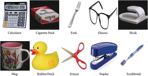
Dataset of this research has total 1440 images with 10 Classes (Figure 2) which are Calculator, Cigarette Pack, Fork, Glasses, Hook, Mug, Rubber Duck, Scissor, Stapler, and Toothbrush, images were taken from Columbia Object Image Library (Nene, Nayar, and Murase 1996). Every image in dataset is RGB and 128 by 128 pixels after pre-processing. One pre-processing requirement is to centering and standardize the data so we divided each pixel value of image by 255. For hyperparameters tuning, we need development set so we split the dataset into training ~60%, development ~20% and testing ~20%.

Figure 2. Dataset for image classification task with ten classes: Calculator, Cigarette Pack, Fork, Glasses, Hook, Mug, Rubber Duck, Scissor, Stapler, and Toothbrush

One of the problem in training deep neural networks is exploding or vanishing gradients so we employed Xavier uniform initializer (Glorot and Bengio 2010) in convolutional layers and fully connected layer to set the initial random weights to resolve the issue of exploding and vanishing gradients to some extent in deep neural networks. We utilized batch normalization (Ioffe and Szegedy 2015) after convolution but before rectified linear unit (ReLU) (Nair and Hinton 2010) activation to normalize hidden units activations and as a result it speed up training process.

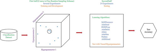
The proposed algorithm consists of two main phases as shown in Figure 3. In first phase, we performed several experiments to come closer to optimal values of hyperparameters as shown in Table 1. The near optimal hyperparameters were selected based on the development set performance of learning algorithms. We selected three best η for each optimizer independently, two M_b, two N_l and two N_e for each method. In second phase, we executed twenty-four final experiments to find the best learning algorithm. In all experiments, we utilized network architecture similar to ResNet (He et al. 2016) of 38 and 50 layers with skip connections over three layers instead of two layers.

Table 1. Eight learning algorithms with their learning rates, mini-batch sizes, number of layers, and number of epochs

Learning algorithms	Learning rates (η)	Mini-batch sizes (Mb)	Number of layers (Nl)	Number of epochs (Ne)
SGDNesterov	0.0009, 0.0015, 0.003	32 and 64	38 and 50	50 and 70
AdaGrad	0.0001, 0.0004, 0.0008
RMSProp	0.000009, 0.00001, 0.00003
AdaDelta	0.03, 0.06, 0.11
Adam	0.00001, 0.00005, 0.0001
AdaMax	0.00007, 0.00015, 0.0004
Nadam	0.00002, 0.00004, 0.00008
AMSGrad	0.0000099, 0.00003, 0.00009

Figure 3. The layout of first and second phases of the proposed algorithm using coarse to fine random sampling scheme

Evaluations

The comparison of training accuracy, development accuracy, training cost, and development cost of learning algorithms of experiment in which the performance of all algorithms are better than their average performance on test set (Table 2) are shown in Figure 4. While the performance on test set of the same experiment of all algorithms can be seen via precision-recall curves (Figure 5) and confusion matrices (Figure 6). We can say that the AdaGrad algorithm outperform the other algorithms with 95.9% accuracy on test set when we set learning rate to 0.0008, mini-batch size to 32, number of layers to 50, and number of epoch to 70.

Figure 4. Accuracy and cost curves of eight learning algorithms on training and development sets. (a) Training accuracy, (b) Development accuracy, (c) Training cost, (d) Development cost

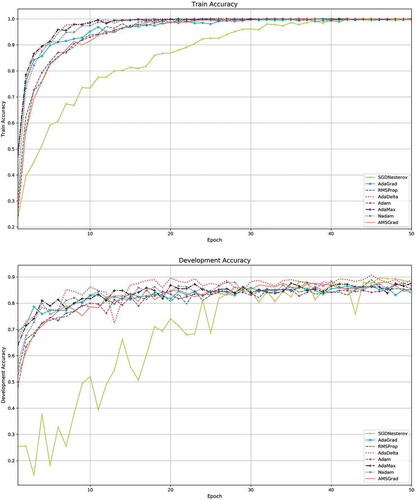
Figure 4. Continued

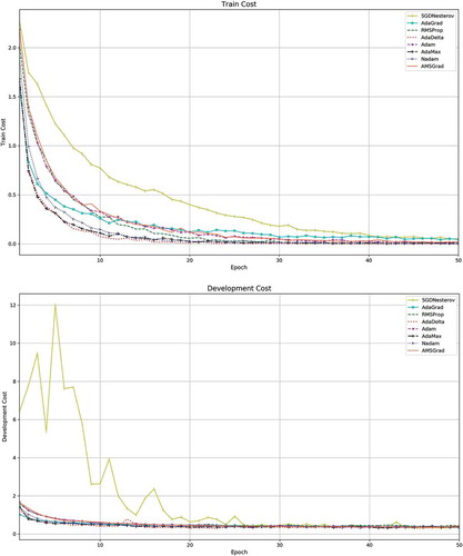
Figure 5. Precision-recall curves of eight learning algorithms on test set of ten object classes. (a) SGDNesterov optimizer, (b) AdaGrad optimizer, (c) RMSProp optimizer, (d) AdaDelta optimizer, (e) Adam optimizer, (f) AdaMax optimizer, (g) Nadam optimizer, (h) AMSGrad optimizer

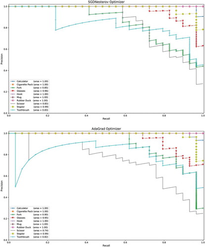
Figure 5. Continued

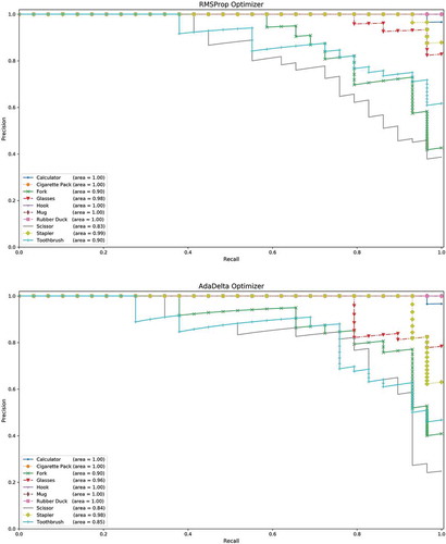
Figure 5. Continued

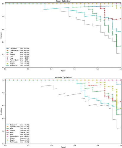
Figure 5. Continued

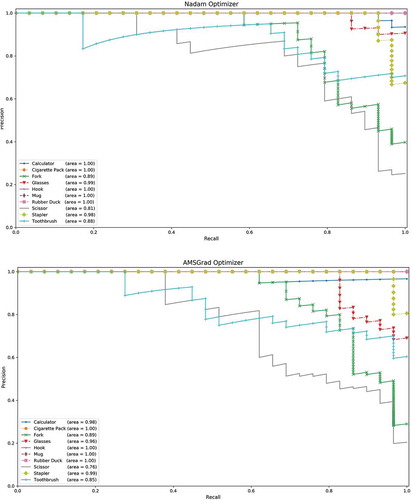
Figure 6. Confusion matrices of eight learning algorithms on test set of ten object classes. (a) SGDNesterov optimizer, (b) AdaGrad optimizer, (c) RMSProp optimizer, (d) AdaDelta optimizer, (e) Adam optimizer, (f) AdaMax optimizer, (g) Nadam optimizer, (h) AMSGrad optimizer

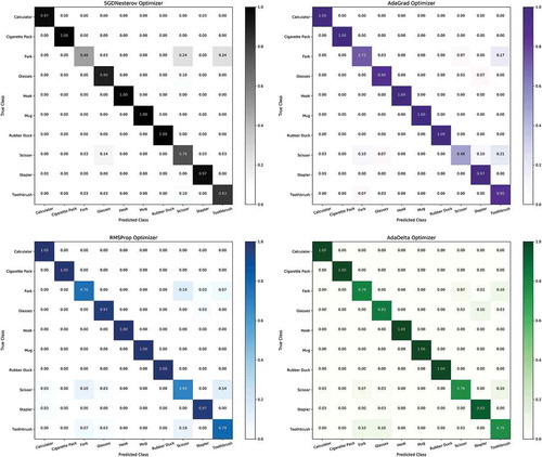
Figure 6. Continued

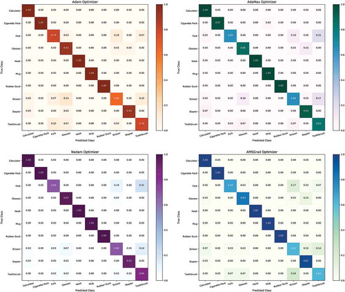
Table 2. Training time, memory utilization, and accuracy on test set of eight learning algorithms. Bold font shows the best results

Learning algorithms	Training time (seconds)		Trained model memory (megabytes)		Accuracy on test set
	Minimum	Maximum	38 Layers architecture	50 Layers architecture	Average	Best
SGDNesterov AdaGrad RMSProp AdaDelta Adam AdaMax Nadam AMSGrad	166 157 161 175 168 164 176 173	365 362 374 418 395 382 418 409	135 135 135 203 203 203 203 270	180 180 180 271 271 271 271 361	0.871 0.889 0.847 0.877 0.882 0.864 0.855 0.857	0.938 0.959 0.917 0.938 0.927 0.941 0.955 0.934

Precision-recall curve is very valuable plot to find which algorithm is performing better. Precision is the number of true positives over the sum of the number of true positives and the number of false positives. Recall is the number of true positives over the sum of the number of true positives and the number of false negatives. A high area under the precision-recall curve denotes high precision as well as high recall, where high recall tells us a low false negative rate, and high precision is simply a low false positive rate.

Confusion matrix (Townsend 1971) is a pictorial way for summarizing the performance of algorithm. Each row of confusion matrix indicates the instances of true class and each column indicates the instances of predicted class. The diagonal entries of confusion matrix show the number for which the predicted class is same as true class, though non-diagonal entries are those which are mislabeled by the algorithm. The higher the diagonal values the better the performance of algorithm.

If we observe Figure 6 carefully, we can see that AdaGrad, RMSProp, AdaDelta, AdaMax, Nadam and AMSGrad wrongly classified a few Scissor images to Toothbrush. We can also see that SGDNesterov, AdaGrad, AdaMax and Nadam algorithms faced difficulty to distinguish between Fork and Toothbrush images. But all algorithms 100% correctly recognized Hook, Mug, and Rubber Duck images.

Best and average accuracies on test set from all twenty-four experiments, maximum and minimum training time to train the networks using each learning algorithms and the memory need to save the trained model in hard disk drive are shown in Table 2. Trained model saving time in hard disk drive for 38 layers’ architecture is around 42 seconds and 50 layers’ architecture is around 72 seconds for all algorithms.

All experiments were performed on GEFORCE GTX1080-8GD5X with CUDA compute capability and last twenty-four experiments took around 17.5 hours. Thirty-eight layers’ architecture has approximately 17.6 million trainable parameters and more than 41 thousand non-trainable parameters. Fifty layers’ architecture has approximately 23.6 million trainable parameters and more than 53 thousand non-trainable parameters.

Conclusions and Future Work

Deep convolutional neural network has become a very useful tool for various scientific research areas nowadays. The goal of this research was to find the best learning algorithm and near optimum hyperparameters values for image classification problem with small dataset. Experiments of this research was divided in two phases. In first phase, several experiments were performed for each learning algorithm to come closer to optimum values of hyperparameters which were tuned for image classification task. The second phase was aimed to determine the best learning algorithm from eight algorithms which were discussed in this research to train the deep networks. After completion of first phase, we selected three best η for each optimizer independently, two M_b, two N_l and two N_e for each technique. We then executed twenty-four final experiments and found that AdaGrad algorithm performed much better when learning rate was 0.0008, mini-batch size was 32, number of layers were 50, and number of epoch were 70 than the rest of the learning algorithms.

For future work, we are aiming to do localization and detection of robotic grasps of objects with deep reinforcement learning as well as work in image processing and guidance for knee and hip replacement surgical robot.

Disclosure Statement

The authors declare that there is no conflict of interests.

Additional information

Funding

This work was supported by the “Chinese Natural Science Research Project” under grant [2017YFC0110700].

References

- Abadi, M.; Agarwal, A.; Barham, P.; Brevdo, E.; Chen, Z.; Citro, C.; Corrado, G.S.; Davis, A.; Dean, J.;Devin, M.; et al. 2016. TensorFlow: Large-scale machine learning on heterogeneous distributed systems. http://arxiv.org/abs/1603.04467.
- Andrej Karpathy, George Toderici, Sanketh Shetty, Thomas Leung, Rahul Sukthankar, Li Fei-Fei. Proceedings of International Computer Vision and Pattern Recognition (CVPR 2014), In 2014, it took place at the Greater Columbus Convention Center in Columbus, Ohio. Main Conference: June 24–27, 2014
- Bengio, Y. 2012. Practical recommendations for gradient-based training of deep architectures. Lecture Notes in Computer Science (Including Subseries Lecture Notes in Artificial Intelligence and Lecture Notes in Bioinformatics), Springer, Berlin, Heidelberg. 7700 LECTU:437–78.
- Collobert, R., and J. Weston. 2008. A unified architecture for natural language processing. Proceedings of the 25th International Conference on Machine Learning, Helsinki, Finland, 2008. http://portal.acm.org/citation.cfm?doid=1390156.1390177.
- Dozat, T. 2016. Incorporating nesterov momentum into adam. ICLR Workshopno 1:2013–16.
- Duchi, J., E. Hazan, and Y. Singer. 2011. Adaptive subgradient methods for online learning and stochastic optimization. Journal of Machine Learning Research 12:2121–59. http://jmlr.org/papers/v12/duchi11a.html.
- Glorot, X., and Y. Bengio. 2010. Understanding the difficulty of training deep feedforward neural networks. Journal of Machine Learning Research 9:249–56.
- He, K., X. Zhang, S. Ren, and J. Sun. 2016 December. Deep residual learning for image recognition. Proceedings of the IEEE Computer Society Conference on Computer Vision and Pattern Recognition. Las Vegas, USA, 770–78.
- Hinton, G., L. Deng, D. Yu, G. E. Dahl, A. Mohamed, N. Jaitly, A. Senior, V. Vanhoucke, P. Nguyen, T. Sainath, et al. 2012. Deep neural networks for acoustic modeling in speech recognition: The shared views of four research groups. IEEE Signal Processing Magazine 29 (6):82–97. http://ieeexplore.ieee.org/abstract/document/6296526/.
- Hinton, G. E., N. Srivastava, and K. Swersky. 2012. Lecture 6a- overview of mini-batch gradient descent. COURSERA: Neural Networks for Machine Learning 31. http://www.cs.toronto.edu/~tijmen/csc321/slides/lecture_slides_lec6.pdf.
- Ioffe, S., and C. Szegedy. 2015. Batch normalization: accelerating deep network training by reducing internal covariate shift. 32nd International Conference on Machine Learning, ICML, 1:448–56.Lille, France. http://arxiv.org/abs/1502.03167.
- Iqbal, I., G. Mustafa, and J. Ma. 2020. Deep learning-based morphological classification of human sperm heads. Diagnostics 10 (5):325. https://www.mdpi.com/2075-4418/10/5/325.
- Iqbal, I., G. Shahzad, N. Rafiq, G. Mustafa, and J. Ma. 2020. Deep learning-based automated detection of human knee joint’s synovial fluid from magnetic resonance images with transfer Learning. IET Image Processing 14 (10):1990–98. doi:10.1049/iet-ipr.2019.1646.
- Iqbal, I., M. Younus, K. Walayat, M. U. Kakar, and J. Ma. 2021. Automated multi-class classification of skin lesions through deep convolutional neural network with dermoscopic images. Computerized Medical Imaging and Graphics 88:101843. doi:10.1016/j.compmedimag.2020.101843.
- Kingma, D. P., and J. L. Ba. 2015. Adam: A method for stochastic optimization. 3rd International Conference on Learning Representations. San Diego, USA. http://arxiv.org/abs/1412.6980.
- Krizhevsky, A., I. Sutskever, and G. E. Hinton. 2012. ImageNet classification with deep convolutional neural networks. Advances in Neural Information Processing Systems 2:1097–105.
- LeCun, Y., L. Bottou, Y. Bengio, and P. Haffner. 1998. Gradient-based learning applied to document recognition. Proceedings of the IEEE 86:2278–323. https://papers.nips.cc/paper/4824-imagenet-classification-with-deep-convolutional-neural-networks.pdf.
- Lecun, Y., Y. Bengio, and G. Hinton. 2015. Deep Learning. Nature 521 (7553):436–44. doi:10.1038/nature14539.
- Mcculloch, W. S., and W. Pitts. 1943. A logical calculus of the ideas immanent in nervous activity. Bulletin of Mathematical Biophysics 5 (4):99–115. doi:10.1007/BF02478259.
- Nair, V., and G. E. Hinton. 2010. Rectified linear units improve restricted boltzmann machines. Proceedings of the 27th International Conference on Machine Learning, Haifa, Palestine. 807–14.
- Nene, S. A., S. K. Nayar, and H. Murase. 1996. Columbia University Image Library. http://www1.cs.columbia.edu/CAVE/software/softlib/coil-100.php
- Nesterov, Y. 1983. A method for unconstrained convex minimization problem with the rate of convergence O (1/K2). Doklady Akademii Nauk SSSR 269 (3):543–47.
- Qian, N. 1999. On the momentum term in gradient descent learning algorithms. Neural Networks 12 (1):145–51. doi:10.1016/S0893-6080(98)00116-6.
- Robbins, H., and S. Monro. 1951. A stochstic approximation method. The Annals of Mathematical Statistics 22 (3):400–07. doi:10.1214/aoms/1177729586.
- Rumelhard, D. E., G. E. Hinton, and R. J. Williams. 1986. Learning representations by back-propagating errors. Letters To Nature 323:533–36. doi:10.1038/323533a0.
- Samuel, A. L. 1959. Some Studies in machine learning using the game of checkers. IBM Journal of Research and Development 3 (3):210–29. doi:10.1147/rd.33.0210.
- Sashank Reddi, Satyen Kale, Sanjiv Kumar. Sixth International Conference on Learning Representations. Vancouver Convention Center, Vancouver CANADA. Mon Apr 30th through May 3rd, 2018
- Simonyan, K., and A. Zisserman. 2015. Very deep convolutional networks for large-scale image recognition. 3rd International Conference on Learning Representations, ICLR 2015 - Conference Track Proceedings. ICLR 2015 held May 7 - 9, 2015 in San Diego, CA.
- Szegedy, C., W. Liu, Y. Jia, P. Sermanet, S. Reed, D. Anguelov, D. Erhan, V. Vanhoucke, and A. Rabinovich. 2015. Going Deeper with Convolutions. Proceedings of the IEEE Computer Society Conference on Computer Vision and Pattern Recognition, 07-12-June:1–9. Boston, USA.
- Townsend, J. T. 1971. Theoretical analysis of an alphabet confusion matrix. Attention Perception & Psychophysics 9 (1A):40–50. doi:10.3758/BF03213026.
- Zeiler, M. D. 2012. ADADELTA: An adaptive learning rate method. http://arxiv.org/abs/1212.5701.