Wind Speed Predictability Accuracy with Height Using LiDAR Based Measurements and Artificial Neural Networks

ABSTRACT

Accurate prediction of future wind speed is important for wind energy integration into the power grid. Wind speeds are usually measured and predicted at lower heights, while modern wind turbines have hub heights of about 80–120 m. As per understanding, this is first attempt to analyze predictability of wind speed with height. To achieve this, wind data was collected using Laser Illuminated Detection and Ranging (LiDAR) system at 10 m, 20 m, 40 m, 90 m, 120 m, 200 m, 250 m and 300 m heights. The collected data is used for training and testing an Artificial Neural Network (ANN) for hourly wind speed prediction for each of the future 12 hours, using 48 previous hourly values. Careful analyses of short term wind speed prediction at different heights and future hours show that wind speed is predicted more accurately at higher heights. For example, the mean absolute percent error decreases from 0.25 to 0.12 corresponding to heights 10 to 300 m, respectively for the 6th future hour prediction, an improvement of around 50%. The performance of ANN method is compared with hybrid genetic algorithm and ANN method namely GANN. Results showed that GANN outperformed ANN for most of the heights for prediction of wind speed at the future 6th hour. Results are also confirmed on another data set and other methods.

Subject classification codes:

• Neural Networks

Introduction

Renewable energy penetration in to the energy mix and wind in particular is increasing globally due to its environmental friendly nature, fast technological development, commercial acceptance, ease of operation and maintenance, and competitive cost. Additionally, the deployment of wind power projects reduce the dependence on fossil fuels and consequently cut down the greenhouse gases (GHG) emissions into the local atmosphere. As a sign of progress in wind power sector, in 2017, the cumulative global wind power installed capacity reached 539.581 GW with new addition of 52.573 GW (2018). At present, there are more than 90 countries contributing toward wind power capacity build up including 9 countries with more than 10 GW and 29 more than 1 GW of installed capacities globally.

Wind speed is a highly fluctuating meteorological parameter both in temporal and spatial domains. It changes with time of the day, month of the year, and also day of the year. This fluctuating nature of wind speed creates an uncertainty in the availability of continuous power and more importantly the stability of the grid. Hence, understanding the variability of the wind speed at a location with time is critical for quality and magnitude of wind energy yield which is directly proportional to the cube of wind speed. It simply means that proper understanding of the wind speed variations based on long term historical wind data and its future trends is a pre-requisite for the success of huge investments. Hence, when planning the deployment of a farm at a site, an indispensable task is to conduct on-site wind speed measurements at least for one complete year (the longer the better) and analyze it to extract information on the variability of the wind (Akdag,et.al 2010; Aksoy, Toprak, and Aytek 2004; Carapellucci and Giordano 2013; Catalão, Pousinho, and Mendes 2011; Chang 2011; Jaramillo and Borja 2004). The variability of wind covers a wide spectrum of time-scales starting from seconds, hours, days, months, year, and to several years. So, predicting the wind speed accurately ahead of time, few hours to days, is important for power producers, grid operators, energy managers, and lastly the consumers (Kaneko et al. 2011). Advance but accurate knowledge of wind speed availability ahead of time can be utilized in applications, such as wind power dispatch planning, power quality, grid operation, reserve allocation, and generation scheduling.

Artificial intelligence techniques such as Artificial Neural Networks (ANN) (Mohandes, Rehman, and Halawani 1998), neuro-fuzzy systems (Mohandes et al. 2007), support vector machines (Mohandes et al. 2004), modes decomposition based low rank multi-kernel ridge regression (Ye et al. 2017), Gaussian process regression combined with numerical weather predictions (Niu et al. 2018), Singular Spectrum Analysis and Adaptive Neuro Fuzzy Inference System (Moreno, Coelho, and Dos 2018), optimal feature selection and a modified bat algorithm with the cognition strategy (Hoolohan, Tomlin, and Cockerill 2018), and spatial model (Naik, Bisoi, and Dash 2018) have been applied to capture the nonlinear trend of the wind speed data series. Since early 2000, trend of using hybrid methodologies has emerged in the literature in which more than one models are combined to achieve better forecasts of wind speed in future and spatial domains (Liu et al. 2010; Liu et al. 2012; Sfetsos 2000). These modern machine learning methods are very useful and provide relatively better estimates both in time and spatial domains as can be seen from wide ranging applications like performance prediction of thermosiphon solar water heaters (Kalogirou, Panteliou, and Dentsoras 1999), analysis of absorption systems (Şencan, Yakut, and Kalogirou 2006), sizing of photovoltaic systems (Mellit, Kalogirou, and Drif 2010, 2010) ground conductivity map generation (Kalogirou et al. 2015), and solar radiation forecasting (Voyant et al. 2017).

Akçay and Filik (2017) developed a framework based on data de-trending, covariance-factorization via subspace method and one and/or multi-step-ahead Kalman filter for the prediction of wind speed. The numerical experiments on the real data sets showed that the wind speed forecast particularly using multi-step-ahead filter outperformed persistence model based predictions. In another study, Filik and Filik (2017) used ANN based models in conjunction with weather parameters like ambient temperature and pressure and found good agreement between the measured and predicted values of wind speed. Santamaría-Bonfil, Reyes-Ballesteros, and Gershenson (2016) predicted wind speeds 1–24 hours ahead using hybrid methodology comprised of Support Vector Regression and showed better forecast compared to persistence and autoregressive models. Hu, Zhang, and Zhou (2016) introduced deep learning neural network technique to predict the wind speed and showed that the proposed approach reduced significantly the error between the predicted and measured values.

Kang et al. (2017) proposed a hybrid Ensemble Empirical Mode Decomposition (EEMD) and Least Square Support Vector Machine (LSSVM) model to improve short-term wind speed forecasting precision. The results showed that the proposed hybrid model outperformed some of the existing methods such as Back Propagation Neural Networks (BP), Auto-Regressive Integrated Moving Average (ARIMA), and combination of Empirical Mode Decomposition (EMD). Liu et al. (2015) used combination of Secondary Decomposition Algorithm (SDA) and the Elman neural networks and showed that the hybrid model performed better than the multi-step wind speed predictions. Wang, Wang, and Wei (2015) showed that Least Square Support Vector Machine and the Markov hybrid model performed better than other models for wind speed prediction. Marović, Sušanj, and Ožanić (2017) proposed ANN based wind speed prediction model for implementation in the early warning system to announce the possibility of the harmful phenomena occurrence due to winds which proved to be accurate in terms of alerting the community ahead of time due to bad wind conditions. Shukur and Lee (2015) used artificial neural network and Kalman filter hybrid model to address the nonlinearity and uncertainty issues and reported to be accurate in comparison with measured values. Jianzhou et al. (2015), used support vector regression combined with seasonal index adjustment and Elman recurrent neural network techniques and obtained relatively better forecast compared to other models.

Koo et al. (2015) evaluated the accuracy of the wind-speed prediction using artificial neural networks in terms of correlation coefficients between actual and simulated wind-speed data for plain, coastal, and mountainous areas. The study concluded that the geographical location played important role in prediction accuracy of wind speed. For hourly prediction, Wu et al. (2015) integrated single multiplicative neuron model with iterated nonlinear filters for updating the wind speed sequence accurately. The results indicated better performance of the proposed model compared to autoregressive moving average, artificial neural network, kernel ridge regression based residual active learning and single multiplicative neuron models. Zhang et al. (2016) used hybrid models (combination of empirical mode decomposition, feature selection with artificial neural network, and support vector machine) for short term wind speed prediction and found better results compared to single ANN, SVM, traditional EMD-based ANN and EMD-based SVM models. Doucoure, Agbossou, and Cardenas (2016) used multi-resolution analysis of the time-series by means of Wavelet decomposition and artificial neural networks and achieved around 29% reduction resources without affecting the predictability. Based on wavelet, wavelet packet, time series analysis, and artificial neural networks, Liu et al. (2013) developed three hybrid models [Wavelet Packet-BFGS, Wavelet Packet-ARIMA-BFGS and Wavelet-BFGS] and compared the performance with Neuro-Fuzzy, ANFIS (Adaptive Neuro-Fuzzy Inference Systems), Wavelet Packet-RBF (Radial Basis Function) and PM (Persistent Model). The results showed that the proposed hybrid models produced better results than the other models.

Most of the above methods use wind speed measurements and predictions at lower heights, while in reality wind energy is generated at hub height. At lower heights, the wind is influenced by ground activities such as heat of the ground, near surface turbulences and human activities. However, at higher heights (more than 80 m) these effects are minimized and better predictions are obtained. This paper utilizes machine learning method to predict wind speeds at different heights and analyses the predictability of wind speed with height. The paper is organized as follows: Section II discusses the methodology, while Section III is devoted to numerical experimental results. Section IV concludes the paper.

Methodology

As the focus of this paper is not the development of a new learning technique, rather our purpose is to analyze the predictability of wind speed with height. Therefore, we used the back propagation (BP) algorithm for training an ANN for short term wind speed prediction at different heights. However, at one specific future hour (6^th hour ahead) we compare the performance of the BP with a hybrid system (GANN) that combines the Genetic Algorithm (GA) with BP to avoid being trapped in local optima. The Application of GA to find optimum initial weights and biases values for ANN has been shown to find a better global solution (Rosin et al. 1997; Doucoure, Agbossou, and Cardenas 2016; Reza 2013). In this paper the GA is used along with the Levenberg-Marquardt (LM) method to enhance the search capability for optimum weights and bias values as illustrated in Figure 1. The LM algorithm is an iterative approach combining gradient descent and Gauss-Newton methods to minimize a function (Marquardt 1963). Parameters change their values every iteration according to the following equation:

(1) $W^{k+1}=W^k-{\left[J^{T}J+\lambda I\right]}^{-1}{J}^T\left(y-\bar{y}\right)$(1)

Figure 1. Training of ANN using genetic algorithm

where $W^{k+1}$and $W^k$are the values of the weights at $(k+1{)}^{th}$and$k^{th}$ iterations, correspondingly. The Jacobian matrix J contains first derivatives of model output with respect to the optimizing parameters. Measured and predicted output values are denoted by$y$and$\bar{y}$, respectively. Increasing the damping parameter$\lambda$decreases the step size, and vice versa. Therefore, if a step is unacceptable, $\lambda$should be increased for a smaller step. If a step is accepted, $\lambda$ is decreased in order to proceed more quickly in the correct descent direction, speeding up the convergence.

For performance evaluation of the proposed method, several measures are used including mean absolute percent error (MAPE), mean square error (MSE), and the coefficient of determination (R²). These error parameters are calculated using the following equations (Rehman 2009):

(2)

(3) $RMSE=\frac{{\sum }_{i=1}^N{\left(M_i-E_i\right)}^2}{N}$(3)

where N is the number of samples, M and E are the measured and the estimated values of the WS.

Experimental Results

The proposed study utilizes hourly averaged WS data collected by LiDAR system between April 2^nd and 30^th June 2015. The data was collected at 10, 20, 40, 90, 120, 200, 250 and 300 m heights above ground level (AGL). Figure 2 shows some measured hourly averaged wind speed data at different heights.

Figure 2. Measured wind speed at 10 m, 90 m and 300 m height

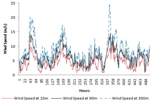
Wind speed at a particular hour is usually correlated with values at previous hours. Initial experiments indicated that using previous 48 hours WS values provide reasonable prediction at the future hours. This study forecasts wind speeds up to 12 hours ahead of time. To carry out this task, 12 different ANN models were built. The first ANN model uses previous 48 hours wind speed values as input to predict the WS at the first future hour as the output. The second model uses the same 48 wind speed values as input to predict the WS at the 2^nd future hour. Similar models were developed to find the wind speed at 3^rd to 12^th future hour using the same previous 48 values as input.

The available data was divided into two parts, training and testing. Wind speed data starting from 2nd April to 20th June was used for training and 21^st June to 30^th June for testing. The number of inputs to the ANN was set to be 48 and the number of output is one in all cases. Single hidden layer with 30 hidden neurons was selected based on the cross validation error analysis. For the GANN model, ten initial populations were considered where each population represents a set of weights and bias values for ANN. Based on cross validation a maximum of 100 iterations, 0.8 crossover factor, and a mutation parameter of 0.01 were found to be the best fit for the model.

Results and Discussions

The present study predicts hourly average wind speeds up to 12 hours ahead at 8 different heights. Separate ANN models are developed for predicting wind speeds at different hours and heights. A hybrid genetic algorithm and neural network method namely GANN (described above) is used to predict each of the future 12 hours ahead at all the heights. The results indicate that MAPE is always less than 0.45 (Table 1). It is also observed that MAPE values decrease with height. For example, for 1 hour predictions, the MAPE values decreased from 0.24 at 10 m to 0.13 at 300 m. Table 2 shows the RMSE between the predicted and measured WS values for each of the future 12 hours at different heights. Data in Table 2 indicates that WS prediction improvement with height is not as obvious as in the case of MAPE. However, it is noticed that RMSE values remain almost the same up to 6 hours predictions. At 10 m, the RMSE values increased from 1.10 to 1.91 m/s corresponding to hours 1 and 12, respectively. Table 3 shows the coefficient of determination R² values between predicted and measured values. The data is an indicative of significant improvements in the prediction of WS with heights in all future hours.

Table 1. MEAN ABSOLUTE PERCENTAGE ERROR (MAPE) AT DIFFERENT HEIGHTS AND DIFFERENT PREDICTION HOURS

	10 m	20 m	40 m	90 m	120 m	200 m	250 m	300 m
1 Hour	0.24	0.21	0.20	0.14	0.16	0.14	0.14	0.13
2 Hour	0.26	0.22	0.22	0.15	0.16	0.14	0.15	0.14
3 Hour	0.23	0.21	0.20	0.17	0.16	0.14	0.13	0.13
4 Hour	0.25	0.23	0.19	0.15	0.17	0.16	0.14	0.13
5 Hour	0.25	0.22	0.20	0.16	0.18	0.16	0.16	0.14
6 Hour	0.25	0.23	0.22	0.16	0.17	0.16	0.14	0.12
7 Hour	0.31	0.26	0.27	0.19	0.19	0.18	0.17	0.15
8 Hour	0.29	0.25	0.26	0.22	0.18	0.18	0.17	0.17
9 Hour	0.37	0.32	0.28	0.22	0.23	0.22	0.20	0.18
10 Hour	0.37	0.33	0.29	0.20	0.22	0.23	0.19	0.18
11 Hour	0.42	0.37	0.33	0.28	0.26	0.26	0.21	0.24
12 Hour	0.40	0.35	0.32	0.30	0.28	0.27	0.23	0.25

Table 2. ROOT MEAN SQUARE ERROR (RMSE) AT DIFFERENT HEIGHTS AND DIFFERENT PREDICTION HOURS

	10 m	20 m	40 m	90 m	120 m	200 m	250 m	300 m
1 Hour	1.10	1.11	1.13	0.91	1.13	1.08	1.16	1.07
2 Hour	1.15	1.15	1.13	0.99	1.13	1.08	1.13	1.20
3 Hour	1.10	1.11	1.17	0.99	1.09	1.08	1.14	1.13
4 Hour	1.15	1.18	1.12	0.97	1.10	1.21	1.08	1.08
5 Hour	1.18	1.13	1.08	1.08	1.17	1.18	1.16	1.13
6 Hour	1.14	1.10	1.13	1.10	1.16	1.23	1.18	1.05
7 Hour	1.30	1.27	1.33	1.27	1.29	1.28	1.32	1.24
8 Hour	1.24	1.27	1.28	1.29	1.31	1.27	1.27	1.31
9 Hour	1.53	1.53	1.56	1.50	1.50	1.61	1.60	1.53
10 Hour	1.59	1.59	1.60	1.48	1.53	1.72	1.58	1.51
11 Hour	1.96	1.83	1.93	1.81	1.96	2.04	1.75	2.03
12 Hour	1.91	1.84	1.87	1.94	1.98	2.03	1.77	1.96

Table 3. COEFFICIENT OF DETERMINATION (R²) AT DIFFERENT HEIGHTS AND DIFFERENT PREDICTION HOURS

	10 m	20 m	40 m	90 m	120 m	200 m	250 m	300 m
1 Hour	0.82	0.87	0.86	0.94	0.90	0.94	0.94	0.95
2 Hour	0.82	0.85	0.86	0.93	0.90	0.95	0.95	0.95
3 Hour	0.82	0.86	0.84	0.93	0.91	0.94	0.94	0.95
4 Hour	0.80	0.83	0.85	0.93	0.91	0.93	0.95	0.96
5 Hour	0.81	0.85	0.87	0.90	0.89	0.93	0.94	0.95
6 Hour	0.81	0.86	0.90	0.89	0.90	0.93	0.94	0.96
7 Hour	0.76	0.80	0.81	0.88	0.87	0.93	0.93	0.94
8 Hour	0.83	0.82	0.84	0.86	0.88	0.93	0.94	0.94
9 Hour	0.67	0.73	0.74	0.82	0.84	0.90	0.89	0.92
10 Hour	0.68	0.70	0.76	0.85	0.83	0.87	0.91	0.91
11 Hour	0.62	0.66	0.67	0.75	0.75	0.83	0.89	0.87
12 Hour	0.59	0.57	0.67	0.70	0.74	0.86	0.88	0.86

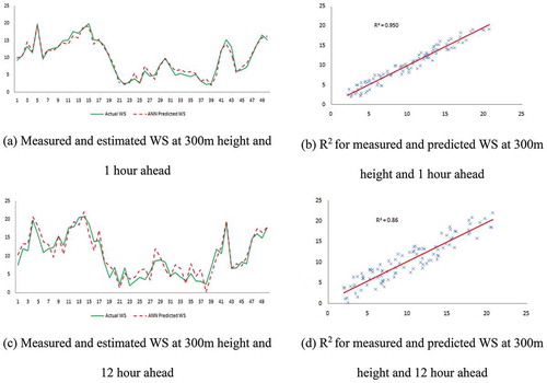
The measured and the predicted WS at 10 m and 1 hour ahead are compared in Figure 3(a). The predicted WS are found to be in close agreement with the measured values and also follow the trend quite closely. The corresponding scatter plot between the measured and predicted WSs at hour 1, Figure 3(b), shows a coefficient of determination of 0.82. The predicted and the measured WSs at 12 hours show relatively poor comparison compared to that for 1 hour ahead of time predictions, Figure 3(c), but do follow the trend quite closely. The scatter diagram, Figure 3(d), resulted in R² value of 0.591. At 90 m, the comparison between the predicted and the measured WS values at 1 hour (Figure 4(a)) is much better than that at 12 hours (Figure 4(c)). However, in both the cases the predicted WSs follow the trends of measured values closely. The scatter plots for 1 hour (Figure 4(b)) and 12 hours ahead of time predictions show less scatter with R² value of 0.936 at 1 hour compared to that at 12 hours with R² value of 0.702. Similar comparisons are made at 120 m and 300 m in Figure 5 and Figure 6, respectively. In all of these cases, it is confirmed that the comparisons between the predicted and measured values at hour 1 are much better than those at 12 hours ahead. This observation is further strengthened by the higher values of R² at 1 hour ahead of time predictions than those at 12 hours ahead.

Figure 3. Performance at height 10 m (a) Measured and predicted WS at 10 m height and 1 hour ahead (b) R² for measured and predicted WS at 10 m height and 1 hour ahead (c) Measured and predicted WS at 10 m height and 12 hour ahead (d) R² for measured and predicted WS at 10 m height and 12 hour ahead

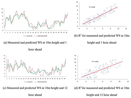
Figure 4. Performance at height 90 m (a) Measured and estimated WS at 90 m height and 1 hour ahead (b) R² for measured and predicted WS at 90 m height and 1 hour ahead (c) Measured and estimated WS at 90 m height and 12 hour ahead (d): R² for measured and predicted WS at 90 m height and 12 hour ahead

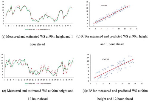
Figure 5. Performance at height 120 m (a) Measured and estimated WS at 120 m height and 1 hour ahead (b) R² for measured and predicted WS at 120 m height and 1 hour ahead (c) Measured and estimated WS at 120 m height and 12 hour ahead (d) R² for measured and predicted WS at 120 m height and 12 hour ahead

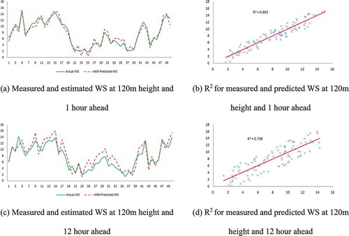
Figure 6. Performance at height 300 m (a) Measured and estimated WS at 300 m height and 1 hour ahead (b) R² for measured and predicted WS at 300 m height and 1 hour ahead (c) Measured and estimated WS at 300 m height and 12 hour ahead (d) R² for measured and predicted WS at 300 m height and 12 hour ahead

ANN and GANN Models Performance Comparison

In this section, the performance of ANN and GANN methods based on the predictions of WS at 6^th future hour and at different heights is compared. The predicted WS values from the two methods are compared with the measurements. The values of the performance measures RMSE, MAPE, and R² for both the methods are summarized in Table 4. The RMSE are around 1.1 m/s in case of ANN approach and always less than 1 m/s in case of GANN method. On the other hand, MAPE values decreased from 0.25 to 0.12 (almost 50%) corresponding to 10 m and 300 m heights; respectively in case of ANN method while these values decreased to 0.11 at 300 m from 0.21 at 10 m (a reduction of almost 48%) in case of GANN approach. Relatively smaller magnitudes of RMSE and MAPE along with the higher values of R² are indicative of better performance of GANN model over ANN approach.

Table 4. COMPARISON BETWEEN ANN AND GANN MODEL BASED ON ESTIMATED WIND SPEED AT 6^TH HOUR AHEAD OF TIME

	RMSE		MAPE		R^2
	ANN	GANN	ANN	GANN	ANN	GANN
10 m	1.14	0.92	0.25	0.21	0.81	0.87
20 m	1.10	0.87	0.23	0.20	0.86	0.91
40 m	1.13	0.89	0.22	0.18	0.90	0.91
90 m	1.10	0.89	0.16	0.14	0.89	0.92
120 m	1.16	0.93	0.17	0.14	0.90	0.93
200 m	1.23	1.01	0.16	0.14	0.93	0.95
250 m	1.18	1.04	0.14	0.13	0.94	0.95
300 m	1.05	0.94	0.12	0.11	0.96	0.97

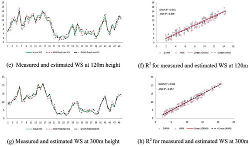
The WS values predicted using the two methods are compared with the measured ones at 10, 90, 120, and 300 m for the 6^th hour and are shown Figure 7. The corresponding scatter plots are also provided in this figure. It is evident from Figure 7(a, c, e, and g) that the comparisons between the predicted and measured WS values keep on improving with increasing height. This fact has also been confirmed by the corresponding scatter plots shown in Figure 7(b, d, f, and h). In these scatter plots, the R² values are found to be larger in case of GANN methods based prediction compared to those based on ANN methodology. Furthermore the coefficient of determination values kept on increasing with height which shows better predictions at higher heights.

Figure 7. Comparison of ANN and GANN at 6^th future hour and different heights (a) Measured and estimated WS at 10 m height (b) R² for measured and estimated WS at 10 m (c): Measured and estimated WS at 90 m height (d) R² for measured and estimated WS at 90 m (e) Measured and estimated WS at 120 m height (f) R² for measured and estimated WS at 120 m (g) Measured and estimated WS at 300 m height (h) R² for measured and estimated WS at 300 m

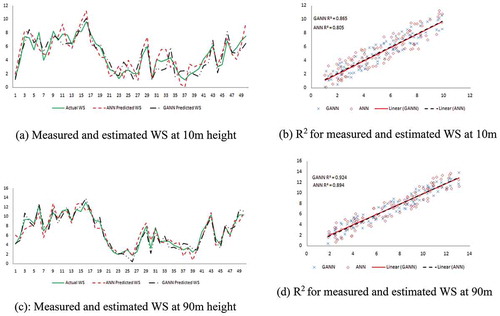
Figure 7. Continued

Predictability Analysis of WS with Heights

This sub-section is devoted to the analysis of the predictability of WS with heights. The MAPE and R² values for WS predictions for each of 1 to 12 hours ahead at each height are compared in Figure 8 using ANN. It is seen that as the prediction period in future time domain increases, the MAPE values also increase (Figure 8(a)). In general, a slower increment is observed in the values of MAPE up to hours 6 and a bit faster at further longer time durations. It is also worth mentioning that as the height of prediction increases, the MAPE value decreases. The R² values remained almost around 0.95 at 200, 250, and 300 m predictions for all the future hours of prediction (Figure 8(b)). At 20 to 120 m heights the R² values between the predicted and the measured WSs are seen to be between 0.8 and 0.9 up to hours 6 and then decreased faster beyond (Figure 8(b)). Figure 9 shows the variation of MAPE and R² with respect to heights using ANN. It can be observed that the performance measures MAPE and R² improve with heights.

Figure 8. Predictability in relation to the future hours (a) Variation of MAPE with prediction hour (b) Variation of R² with prediction hour

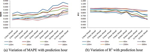
Figure 9. Predictability with heights (a) Variation of MAPE with respect to height (a) Variation of MAPE with heights (b) Variation of R² with heights

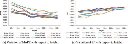
(A) Variation of R² with respect to Height

To further validate the results, we analyzed the predictability of wind speed with height using another data set. This data set represents hourly averaged WS collected by LiDAR system between 20 June 2015 and 29 February 2016. The data is collected at 10, 80, 120, 160 and 180 m heights AGL. Furthermore, we compared the performances of several methods, namely, ANN, GANN, Support Vector Machine for regression (SVMR), and Auto-Regressive model (AR). For the machine learning methods, we used the same number of layers and units as used in the first data set. The MAPE and R² values for WS predictions for 1 hour ahead at each height using all methods and the average performance of all methods are shown in Figure 10. The figures confirm the results obtained with the first data set that predictability of wind speed improves with heights. The MAPE values on average show a decreasing pattern with increasing heights. Additionally, the R² values increase with increasing height, an indication of improved predictability.

Figure 10. Predictability in relation to the heights for the second data set

Conclusions

The knowledge of future wind speed is helpful for the estimation of available wind power which is critical for utility grid planning and operation. Typically, wind speed measurements and prediction are performed at low heights (10–40 m). Modern wind turbines operate at hub heights (80–120 m). For the first time, to the best knowledge of the authors, this paper assessed the predictability of wind speed relative to heights. LiDAR device was deployed to collect hourly averaged wind speed data and machine learning method was used for short term prediction. Artificial neural networks (ANN) were used to predict wind speeds at each of the 12 hours ahead of time based on previous 48 hours. Predicted future values from 1^st to the 6^th hour did not deteriorate significantly (at height 120 m MAPE ranged between 0.16–0.17) compared to the 7^th to the 12^th future hours (MAPE is increased up to 0.28).

It was observed that the predictability of wind speed improves with increasing heights. The MAPE values improved from 0.25 at 10 m height to 0.17 at 120 m and further reduced to 0.12 at 300 m for sixth hour future wind speed prediction. For 12th hour future predictions, these values decrease from 0.40 to 0,28, and 0.25 corresponding to heights, 10, 120, 300 m, respectively. The coefficient of determination R² for the 6^th hour prediction is improved from 0.81 to 0.90 and 0.96 corresponding to heights 10, 120, 300 m, respectively. The used method is compared with a hybrid genetic algorithm and neural network method namely GANN on the prediction of WS at different heights for the 6^th future hour. Comparison showed that the GANN performed better than ANN in terms of all performance measures. The improved predictability of WS with heights is validated on another data set with other methods (ANN, GANN, SVMR, and AR) as well.

Acknowledgments

This research was funded by the Deanship of Scientific Research, King Fahd University of Petroleum & Minerals (KFUPM) award number DF191024

References

- Akçay, H., and T. Filik. 2017. Short-term wind speed forecasting by spectral analysis from long-term observations with missing values. Applied Energy 191:653–62. doi:10.1016/j.apenergy.2017.01.063.
- Akdag˘, S. A., H. S. Bagiorgas, and G. Mihalakakou. 2010. Use of two-component Weibull mixtures in the analysis of wind speed in the Eastern Mediterranean. Applied Energy 87 (8):2566–73. doi:10.1016/j.apenergy.2010.02.033.
- Aksoy, H., Z. F. Toprak, and A. Aytek. 2004. Unal NE. Stochastic generation of hourly mean wind speed data. Renewable Energy 29 (14):2111–31. doi:10.1016/j.renene.2004.03.011.
- Carapellucci, R., and L. Giordano. 2013. The effect of diurnal profile and seasonal wind regime on sizing grid-connected and off-grid wind power plants. Applied Energy 107:364–76. doi:10.1016/j.apenergy.2013.02.044.
- Catalão, J. P. S., H. M. I. Pousinho, and V. M. F. Mendes. 2011. Short-term wind power forecasting in Portugal by neural networks and wavelet Transform. Renewable Energy 36 (4):1245–51. doi:10.1016/j.renene.2010.09.016.
- Chang, T. P. 2011. Performance comparison of six numerical methods in estimating Weibull parameters for wind energy application. Applied Energy 88 (1):272–82. doi:10.1016/j.apenergy.2010.06.018.
- Doucoure, B., K. Agbossou, and A. Cardenas. 2016. Time series prediction using artificial wavelet neural network and multi-resolution analysis: Application to wind speed data. Renewable Energy 92:202–11. doi:10.1016/j.renene.2016.02.003.
- Filik, Ü. B., and T. Filik. 2017. Wind Speed Prediction Using Artificial Neural Networks Based on Multiple Local Measurements in Eskisehir. Energy Procedia 107 (February):264–69. doi:10.1016/j.egypro.2016.12.147.
- Global Wind Report 2017 – Annual market update (GWEC-2017), http://gwec.net/wp-content/uploads/vip/GWEC_PRstats2017_EN-003_FINAL.pdf ( Accessed on 3rd Ma 2018)
- Hoolohan, V., A. S. Tomlin, and T. Cockerill. 2018. Improved near surface wind speed predictions using Gaussian process regression combined with numerical weather predictions and observed meteorological data. Renewable Energy 126:1043–54. doi:10.1016/j.renene.2018.04.019.
- Hu, Q., R. Zhang, and Y. Zhou. 2016. Transfer learning for short-term wind speed prediction with deep neural networks. Renewable Energy 85:83–95. doi:10.1016/j.renene.2015.06.034.
- Jaramillo, O. A., and M. A. Borja. 2004. Winds peed analysis in La Ventosa, Mexico: A bimodal probability distribution case. Renewable Energy 29 (10):1613–30. doi:10.1016/j.renene.2004.02.001.
- Jianzhou, W. J., S. Qin, Q. Zhou, and H. Jiang. 2015. Medium-term wind speeds forecasting utilizing hybrid models for three different sites in Xinjiang, China. Renewable Energy 76 (4):91–101. doi:10.1016/j.renene.2014.11.011.
- Kalogirou, S. A., G. A. Florides, P. D. Pouloupatis, P. Christodoulides, and J. Joseph-Stylianou. 2015. Artificial neural networks for the generation of a conductivity map of the ground. Renewable Energy 77:400–07. doi:10.1016/j.renene.2014.12.033.
- Kalogirou, S. A., S. Panteliou, and A. Dentsoras. 1999. Artificial neural networks used for the performance prediction of a thermosiphon solar water heater. Renewable Energy 18 (1):87–99. doi:10.1016/S0960-1481(98)00787-3.
- Kaneko, T., A. Uehara, T. Senjyu, A. Yona, and N. Urasaki. 2011. An integrated control method for a wind farm to reduce frequency deviations in a small power system. Applied Energy 88 (4):1049–58. doi:10.1016/j.apenergy.2010.09.024.
- Kang, A., Q. Tan, X. Yuan, X. Lei, and Y. Yuan, Short-Term Wind Speed Prediction Using EEMD-LSSVM Model, Advances in Meteorology Volume 2017, Article ID 6856139, 22 pages.
- Koo, J., G. D. Han, H. J. Choi, and J. H. Shim. 2015. Wind-speed prediction and analysis based on geological and distance variables using an artificial neural network: A case study in South Korea. Energy 93:1296–302. doi:10.1016/j.energy.2015.10.026.
- Liu, H., C. Chen, H. Qi Tian, and Y. Fei Li. 2012. A hybrid model for wind speed prediction using empirical mode decomposition and artificial neural networks. Renew. Energy 48:545–56. (0). doi:10.1016/j.renene.2012.06.012.
- Liu, H., H. Tian, D. Pan, and Y. Li. 2013. Forecasting models for wind speed using wavelet, wavelet packet, time series and Artificial Neural Networks. Applied Energy 107:191–208. doi:10.1016/j.apenergy.2013.02.002.
- Liu, H., H. Tian, X. Liang, and Y. Li. 2015. Wind speed forecasting approach using secondary decomposition algorithm and Elman neural networks. Applied Energy 157 (11):183–94. doi:10.1016/j.apenergy.2015.08.014.
- Liu, H., H.-Q. Tian, and C. Chen. fei Li Y. 2010.A hybrid statistical method to predict wind speed and wind power, Renew. Energy 358:1857–1861. 10.1016/j.renene.2009.12.011
- Marović, I., I. Sušanj, and N. Ožanić, Development of ANN Model for Wind Speed Prediction as a Support for Early Warning System, Complexity Volume 2017, Article ID 3418145, 10 pages.
- Marquardt, D. W. 1963. An algorithm for least-squares estimation of nonlinear parameters. Journal for the Society Industrial and Applied Mathematics 11 (2):431–41. doi:10.1137/0111030.
- Mellit, A., S. A. Kalogirou, and M. Drif. 2010. Application of neural networks and genetic algorithms for sizing of photovoltaic systems. Renewable Energy 35 (12):2881–93. doi:10.1016/j.renene.2010.04.017.
- Mohandes, M., S. Rehman, and T. Halawani. 1998. A neural networks approach for wind speed prediction. Renew. Energy 13 (3):345–54. doi:10.1016/S0960-1481(98)00001-9.
- Mohandes, M., T. Halawani, S. Rehman, and A. A. Hussain. 2004. Support vector machines for wind speed prediction. Renew. Energy 29 (6):939–47. doi:10.1016/j.renene.2003.11.009.
- Mohandes, M., T. Halawani, S. Rehman, and A. A. Hussain. 2007. A locally recurrent fuzzy neural network with application to the wind speed prediction using spatial correlation. Neurocomputing 70 (79):1525–42. doi:10.1016/j.neucom.2006.01.032.
- Moreno, S. R., L. Coelho, and S. Dos. 2018. Wind speed forecasting approach based on Singular Spectrum Analysis and Adaptive Neuro Fuzzy Inference. System, Renewable Energy 126:736–54. doi:10.1016/j.renene.2017.11.089.
- Naik, J., R. Bisoi, and P. K. Dash. 2018. Prediction interval forecasting of wind speed and wind power using modes decomposition based low rank multi-kernel ridge regression. Renewable Energy 129:357–83. doi:10.1016/j.renene.2018.05.031.
- Niu, T., J. Wang, K. Zhang, and P. Du. 2018. Multi-step-ahead wind speed forecasting based on optimal feature selection and a modified bat algorithm with the cognition strategy. Renewable Energy 118:213–29. doi:10.1016/j.renene.2017.10.075.
- Rehman, S. 2009. Empirical Model Development and Comparison with Existing Correlations. Applied Energy 64 (1–4):369–78. doi:10.1016/S0306-2619(99)00108-7.
- Reza, T. 2013. Comparison result of inversion of gravity data of a fault by particle swarm optimization and levenberg-marquardt methods. Springer Plus. doi:10.1186/2193-1801-2-462.
- Rosin, C. D., Halliday, R. S., Hart, W. E., R.K. Below, R. K.1997. A comparison of global and local search methods in drug docking. In Proceedings of the seventh International Conference on Genetic Algorithms:221-229. T. Baeck, Ed., Morgan Kaufmann, Pub. San Francisco, CA.
- Santamaría-Bonfil, G., A. Reyes-Ballesteros, and C. Gershenson. 2016. Wind speed forecasting for wind farms: A method based on support vector regression. Renewable Energy 85 (1):790–809. doi:10.1016/j.renene.2015.07.004.
- Şencan, A., K. A. Yakut, and S. A. Kalogirou. 2006. Thermodynamic analysis of absorption systems using artificial neural network. Renewable Energy Pages. 31 (1):29–43. doi:10.1016/j.renene.2005.03.011.
- Sfetsos, A. 2000. A comparison of various forecasting techniques applied to mean hourly wind speed time series. Renew. Energy 21 (1):23–35. doi:10.1016/S0960-1481(99)00125-1.
- Shukur, O. B., and M. H. Lee. 2015. Daily wind speed forecasting through hybrid KF-ANN model based on ARIMA. Renewable Energy 76 (4):637–47. doi:10.1016/j.renene.2014.11.084.
- Voyant, C., G. Notton, S. A. Kalogirou, N. Marie-Laure, C. Paoli, F. Motte, and A. Fouilloy. 2017. Machine learning methods for solar radiation forecasting: A review. Renewable Energy 105:569–82. doi:10.1016/j.renene.2016.12.095.
- Wang, Y., J. Wang, and X. Wei. 2015. A hybrid wind speed forecasting model based on phase space reconstruction theory and Markov model: A case study of wind farms in northwest China. Energy 91 (11):556–72. doi:10.1016/j.energy.2015.08.039.
- Wu, X., Z. Zhu, X. Su, S. Fan, Z. Du, Y. Chang, and Q. Zeng. 2015. A study of single multiplicative neuron model with nonlinear filters for hourly wind speed prediction. Energy 88:194–201. doi:10.1016/j.energy.2015.04.075.
- Ye, L., Y. Zhao, C. Zeng, and C. Zhang. 2017. Short-term wind power prediction based on spatial model. Renewable Energy 101:1067–74. doi:10.1016/j.renene.2016.09.069.
- Zhang, C., H. Wei, J. Zhao, T. Liu, T. Zhu, and K. Zhang. 2016. Short-term wind speed forecasting using empirical mode decomposition and feature selection. Renewable Energy 96:727–37. doi:10.1016/j.renene.2016.05.023.