Horse Herd Optimization Algorithm for Fuel Constrained Day-ahead Scheduling of Isolated Nanogrid

ABSTRACT

Day-ahead scheduling of isolated nanogrid (NG) is an important task in power system. Owing to slowly lessening of fossil fuel, the profitable use of available fuel for electric power generation has turn out to be an extremely important concern of electric power utilities. This paper suggests horse herd optimization algorithm (HOA) to solve fuel constrained day-ahead scheduling of isolated nanogrid (NG) for five neighboring homes. NG comprises diesel generators, solar PV plants, battery energy storage system (BESS) and plug-in electric vehicles (PEVs). Simulation results of the test system have been compared with those obtained from social group entropy optimization, self-organizing hierarchical particle swarm optimizer with time-varying acceleration coefficients, fast convergence evolutionary programming and differential evolution. It has been observed from the comparison that the suggested HOA has the capacity to give better solution.

Introduction

The local electric power generation and utilization plays a vital role in the electric power system reenactment. Nanogrids (NGs) are very small-scale, low-voltage electricity systems consisting of distributed energy resources for example renewable and nonrenewable distributed generators, battery energy storage systems, and controllable loads.

Fossil fueled fired power plants are the major sources of power generation till now. Owing to slow lessening of fossil fuel, there is concern over fossil fuel scarcity. Fuel suppliers have enforced additional restrictions on fuel supplying agreement and electric power utility has been forced to reschedule power generation anchored in the fuel availability.

Trefny et al. (1981) have explicated economic dispatch problem taking into account fuel constraints. Fuel resource scheduling in energy management has been described by Vemuri, Hackett, and Lugtu (1984) and Kumar et al. (1984).

Burmester et al. (2017) have described about NG technologies. Akinyele and Akinyele (2017) has described design as well as performance analysis of NG. Lee et al. (2019) have discussed about optimum power management for NG. Dahiru and Tan (2020) have discussed about optimum sizing and analysis of grid-connected NG.

NG can operate in grid-connected mode and islanded mode. In grid-connected mode, the NG can swop power with the grid but in islanded mode, there is no grid for swopping power. Therefore in islanded mode owing to erratic nature of renewable energy sources, battery energy storage device is used to increase the system dependability in power shortfall situation.

Alipour, Moradi-Dalvand, and Zare (2017) and Aliasghari et al. (2018) have described PEVs as an electric load while batteries are charging and automobiles get energy from the system i.e. grid-to-vehicle mode. PEV owners can achieve lesser charging cost through competent management and controlling of batteries charging by taking part in time of use (TOU) program as a bendable load.

Kumar et al. (2019) have developed and applied modified symbiotic organisms search (MSOS) algorithm with six truss design problems. Kumar et al. (2020) have applied five improved metaheuristics i.e. improved dragonfly algorithm, improved whale optimization algorithm, improved ant lion optimizer, improved heat transfer search, and improved teaching–learning-based optimization and simulated annealing for truss optimization. Tejani, Kumar, and Gandomi (2019) have applied multi-objective heat transfer search algorithm (MHTS) for truss optimization. Kumar et al. (2020) have developed and applied multi-objective heat transfer search with modified binomial crossover (MOHTS-BX) for multi-objective truss optimization problems. Kumar et al. (2021b) have developed multi-objective hybrid heat transfer search and passing vehicle search optimizer (MOHHTS–PVS) and applied this algorithm for multi-objective structural optimization problem. Kumar et al. (2021a) have developed physics-based multi-objective plasma generation optimizer (MOPGO) and applied this algorithm to solve structural optimization problems. Kumar et al. (2020) have developed multi-objective passing vehicle search (MOPVS) algorithm and applied for structural design optimization problem.

Swarm Intelligence (SI) imitates the group behavior of animals consisting of several agents functioning jointly. In very recent times, MiarNaeimi et al. (2021) has established horse herd optimization algorithm (HOA). HOA is based on the social recitals of different ages of horses utilizing six significant traits. These are lesion, pecking order, amicability, emulation, protection mechanism and meander.

In this article, the problem of fuel constrained day-ahead scheduling in an isolated NG with demand side management (DSM) is formulated. NG consists of diesel generators, solar PV plants, battery energy storage system (BESS) and plug-in electric vehicles (PEVs).

The problem is solved with and without fuel constraints by utilizing suggested HOA, social group entropy optimization (SGEO), self-organizing hierarchical particle swarm optimizer with time-varying acceleration coefficients (HPSO-TVAC), fast convergence evolutionary programming (FCEP) and differential evolution (DE).

A test system containing two diesel generators, two solar PV plants, one battery energy storage system (BESS) and five plug-in electric vehicles (PEVs) is considered to simulate fuel constrained day-ahead scheduling with DSM. It is seen that the suggested HOA proffers better-quality solution.

The major contributions of this manuscript can be stated as follows:

• Day-ahead scheduling of isolated NG comprising diesel generators, solar PV plants, BESS and PEVs has been presented.

• Uncertainty of solar PV plants has been taken into consideration.

• Fuel constraints and ramp rate limit constraints of diesel generators have been considered.

• Demand side management has been taken into consideration.

• The problem is solved with and without fuel constraints.

• Horse herd optimization algorithm has been used to solve the problem.

Problem formulation

The main objective is to find out fuel constrained day-ahead scheduling of isolated NG with DSM. The system considers diesel generators, BESS and PEVs. Mathematical formulation of the problem is affirmed as:

Objective function

(1) $C_{\mathrm{T}}=\sum _{t=1}^{\mathrm{T}}\left[\sum _{i=1}^{{\mathrm{N}}_d}fd{g}_{it}\left(\mathrm{P}d{g}_{it}\right)+\sum _{j=1}^{{\mathrm{N}}_{PV}}fp{v}_{jt}\left(\mathrm{P}p{v}_{jt}\right)\right]$(1)

Fuel price function of $i$th diesel generating unit at time $t$ is affirmed as

(2) $fd{g}_{it}\left(\mathrm{P}d{g}_{it}\right)=a_{di}+b_{di}\mathrm{P}d{g}_{it}+c_{di}\mathrm{P}d{g}_{it}^2$(2)

The cost of solar power as described by Liang and Liao (2007) consists of three terms, a direct cost, an under estimation penalty cost ($Upv$) and an over estimation reserve cost ($Opv$) of solar power.

(3) $fp{v}_{kt}\left(\mathrm{P}p{v}_{kt}\right)=\mathrm{K}p{v}_k\times \mathrm{P}p{v}_{kt}+Op{v}_{kt}\left(\mathrm{P}p{v}_{kt}\right)+Up{v}_{kt}\left(\mathrm{P}p{v}_{kt}\right)$(3)

The overestimation reserve cost and underestimation penalty cost on solar power is replicated as in (4)-(5) respectively.

(4) $Op{v}_{kt}\left(\mathrm{P}p{v}_{kt}\right)=op{v}_k\times \underset{\mathrm{P}p{v}_{kt}^{min}}{\overset{\mathrm{P}p{v}_{kt}}{\int }}\left(\mathrm{P}p{v}_{kt}-x\right)\times fpv\left(x\right)dx$(4)

(5) $Up{v}_{kt}\left(\mathrm{P}p{v}_{kt}\right)=up{v}_k\times \underset{\mathrm{P}p{v}_{kt}}{\overset{\mathrm{P}p{v}_{kt}^{max}}{\int }}\left(x-\mathrm{P}p{v}_{kt}\right)\times fpv\left(x\right)dx$(5)

Constraints

(i) Power balance constraints

(6) $\sum _{i=1}^{{\mathrm{N}}_d}\mathrm{P}d{g}_{it}+\sum _{j=1}^{{\mathrm{N}}_{PV}}\mathrm{P}p{v}_{jt}+\mathrm{P}ESS{D}_t-\sum _{l=1}^{{\mathrm{N}}_{EV}}{\mathrm{P}}_{EVlt}-\left(1-D{r}_t\right)\times L_{Base,t}-L{s}_t=0,t\in \mathrm{T}$(6)

(7) $\sum _{i=1}^{{\mathrm{N}}_d}\mathrm{P}d{g}_{it}+\sum _{j=1}^{{\mathrm{N}}_{PV}}\mathrm{P}p{v}_{jt}-\mathrm{P}ESS{C}_t-\sum _{l=1}^{{\mathrm{N}}_{EV}}{\mathrm{P}}_{EVlt}-\left(1-D{r}_t\right)\times L_{Base,t}-L{s}_t=0,t\in \mathrm{T}$(7)

Equation (6)(6) $\sum _{i=1}^{{\mathrm{N}}_d}\mathrm{P}d{g}_{it}+\sum _{j=1}^{{\mathrm{N}}_{PV}}\mathrm{P}p{v}_{jt}+\mathrm{P}ESS{D}_t-\sum _{l=1}^{{\mathrm{N}}_{EV}}{\mathrm{P}}_{EVlt}-\left(1-D{r}_t\right)\times L_{Base,t}-L{s}_t=0,t\in \mathrm{T}$(6) is applicable when battery is discharging mode and equation (7)(7) $\sum _{i=1}^{{\mathrm{N}}_d}\mathrm{P}d{g}_{it}+\sum _{j=1}^{{\mathrm{N}}_{PV}}\mathrm{P}p{v}_{jt}-\mathrm{P}ESS{C}_t-\sum _{l=1}^{{\mathrm{N}}_{EV}}{\mathrm{P}}_{EVlt}-\left(1-D{r}_t\right)\times L_{Base,t}-L{s}_t=0,t\in \mathrm{T}$(7) is applicable when battery is charging mode.

Solar power model

The power output as described by Shilaja et al. (2017) from $j$th solar PV plant at time $t$ is avowed by

${\mathrm{P}}_{PVjt}={{\mathrm{P}}_{PVr}}_j\times \left[1+\alpha \times \left({\mathrm{T}}_{ref}-\mathrm{T}am{b}_t\right)\right]\times \frac{G}{1000}$, $j\in {\mathrm{N}}_{PV}$, $t\in \mathrm{T}$ (8)

Battery energy storage system

The battery energy storage system (BESS) can provide power at any time when the state of charge $\left(SOC\right)$ is more than the minimum allowable value ${\left(SOC\right)}_{min}$. The SOC of BESS in next hour hinges on SOC and net charging power in the present hour and it is devised as

(9) ${\left(SOC\right)}_{\left(t+1\right)}={\left(SOC\right)}_t+PESS{C}_t\times \eta -\mathrm{P}ESS{D}_t$(9)

SOC of a BESS must be always less than ${\left(SOC\right)}_{max}$and more than ${\left(SOC\right)}_{min}$.

(10) ${\left(SOC\right)}_{min}\le {\left(SOC\right)}_t\le {\left(SOC\right)}_{max}$(10)

The power by which BESS can be charged is limited by maximum charging power limit $\mathrm{P}c{h}_{max}$.

(11) $\mathrm{P}ESS{C}_t\le \mathrm{P}c{h}_{max}$(11)

The power by which BESS can be discharged is limited by maximum discharging power limit $\mathrm{P}di{s}_{max}$.

(12) $\mathrm{P}ESS{D}_t\le \mathrm{P}di{s}_{max}$(12)

PEV charging power limit

The PEV charging/discharging power in each hour is limited by the charging/discharging facility and the energy requirement.

(13) $\sum _{t=1}^{\mathrm{T}}{\mathrm{P}}_{PEVlt}={\mathrm{P}}_{PEVl,total}$(13)

The power necessary of the $n$th PEV is the total power ${\mathrm{P}}_{PEVl,total}$ which has to be charged in a one day time horizon and computed by the average mileage of commuter vehicles for normal personal use. The charging/discharging facility is limited by the maximum and minimum charging/discharging power of PEV. Here, charging-only mode of PEV is considered. Power delivered to PEVs is modeled as real-valued variable. This is due to fact that the delivered power for a single PEV in an hour horizon is easily adjusted through controlling the charging time period. The majority of vehicles (about 90%) is averagely idle or off road along the all day time horizon. PEVs can plug-in to the microgrid when they are not in use. The operational features PEV include the energy demand, min/max capacity and state of charge (SOC) of batteries. The acquired charging power of$n$th PEV from the microgrid is subjected to the charging capacity constraints represented by Eq. (14)(14) ${\mathrm{P}}_{EVl}^{min}\le {\mathrm{P}}_{EVlt}\le {\mathrm{P}}_{EVl}^{max}$(14) .

(14) ${\mathrm{P}}_{EVl}^{min}\le {\mathrm{P}}_{EVlt}\le {\mathrm{P}}_{EVl}^{max}$(14)

(ii) Capability frontiers of diesel generators

(15) $\mathrm{P}d{g}_i^{min}\le \mathrm{P}d{g}_{it}\le \mathrm{P}d{g}_i^{max},i\in {\mathrm{N}}_d,t\in \mathrm{T}$(15)

(iii) Ramp rate limits constraints of diesel generators

(16) $\mathrm{P}d{g}_{it}-\mathrm{P}d{g}_{i(t-1)}\le U{R}_{di},i\in {\mathrm{N}}_d,t\in \mathrm{T}$(16)

(17) $\mathrm{P}d{g}_{i(t-1)}-\mathrm{P}d{g}_{it}\le D{R}_{di},i\in {\mathrm{N}}_d,t\in \mathrm{T}$(17)

(iv) Fuel delivery constraints of diesel generators

Total fuel delivered to all diesel generating units should balance the fuel supplied by the supplier at every intermission over the scheduling horizon

$\sum _{i=1}^{{\mathrm{N}}_d}Fd{g}_{im}-F{D}_{dm}=0$, $m\in \mathrm{M}$ (18)

(V) Fuel Storage Constraints of Diesel Generators

The fuel volume of every diesel generating unit at the starting of every intermission plus fuel delivered to that diesel generating unit minus the fuel smoldered at that diesel generating unit provides the residual fuel at the starting of the next intermission.

$Vd{g}_{im}=Vd{g}_{i\left(m-1\right)}+Fd{g}_{im}$ -$\sum _{t=1}^{t_m}\left[{\eta }_{di}+{\delta }_{di}\mathrm{P}d{g}_{it}+{\mu }_{di}\mathrm{P}d{g}_{it}^2\right]$,$i\in {\mathrm{N}}_d$,$m\in \mathrm{M}$ (19)

(Vi) Fuel Delivery Limits of Diesel Generators

Fuel delivered to every diesel generating unit at every intermission must be inside its minimum limit $Fd{g}^{min}$ and maximum limit $Fd{g}^{max}$.

$Fd{g}_i^{min}\le Fd{g}_{im}\le Fd{g}_i^{max}$, $i\in {\mathrm{N}}_d$, $m\in \mathrm{M}$ (20)

(Vii) Fuel Storage Limits of Diesel Generators

Fuel storage limit of every diesel generating unit at every intermission must be inside its minimum limit $Vd{g}^{min}$ and maximum limit $Vd{g}^{max}$.

$Vd{g}_i^{min}\le Vd{g}_{im}\le Vd{g}_i^{max}$, $i\in {\mathrm{N}}_d$, $m\in \mathrm{M}$ (21)

Demand side management

Demand side management (DSM) programs as described by Morsali et al. (2018) has several merits for example reducing the cost, boosting the power system security [12], etc. The DSM programs are categorized as demand response, strategic conservation etc. Here, demand response program is employed and it is modeled according to time-of-use (TOU) program, where some percentage of load demand is budged from expensive period cheap period keeping the total amount of load demand to be fixed. As a result, load curve is flattened and the operation cost is trimmed down. The numerical model of TOU program is described according to the equation (22)(22) $L_t=\left(1-D{R}_t\right)\times L_{Base}+L_{st}$(22) constrained by equations (23)(23) $\sum _{t=1}^{\mathrm{T}}{L}_{st}=\sum _{t=1}^{\mathrm{T}}D{R}_t\times L_{Base,t}$(23) -(26).

(22) $L_t=\left(1-D{R}_t\right)\times L_{Base}+L_{st}$(22)

(23) $\sum _{t=1}^{\mathrm{T}}{L}_{st}=\sum _{t=1}^{\mathrm{T}}D{R}_t\times L_{Base,t}$(23)

(24) $L_{In{c}_t}=In{c}_t\times L_{Base,t}$(24)

$D{R}_t\le D{R}^{max}$,$t\in \mathrm{T}$ (25)

$In{c}_t\le In{c}^{max}$, $t\in \mathrm{T}$(26)

Horse herd optimization algorithm

Horse herd optimization algorithm (HOA) developed by MiarNaeimi et al. (2021) is founded on the behavioral pattern of horses in their day to day life. The behavioral pattern of horses usually includes lesion, pecking order, amicability, emulation, protection mechanism and meander. HOA technique is motivated by these behaviors of horses at different ages. The movement of horses emulated in HOA during each iteration is given by

${\mathrm{X}}_k^{Age,Itr}={\mathrm{X}}_k^{Age,(Itr-1)}+{\bar{V}}_k^{Age,Itr}$, $Age=\alpha ,\beta ,\gamma ,\delta$ (27)

where, ${\mathrm{X}}_k^{Age,Itr}$ signifies the position of the $k$th horse, $Age$ and ${\bar{V}}_k^{Age,Itr}$demonstrate the age range and velocity vector of the considered horse, $Itr$ is the current iteration.

Horses show dissimilar behaviors at different ages. The highest natural life of a horse is about 25–30 years. δ signifies horses at era range of 0–5 years, γ signifies horses at range of 5–10 years, β signifies horses era range of 10–15 years, and α signifies horses older than 15 years.

Horses are sorted founded on the best responses. Therefore, first 10% of horses from top of sorted matrix have been chosen as α horses. Next 20% have been in β group. γ and δ horses account for 30% and 40% of residual horses, respectively. Six behaviors of horses are precisely applied for detecting velocity vector. Velocity vector of horses at dissimilar eras during every cycle of method is confirmed as

(28) ${\bar{V}}_k^{\alpha ,Itr}={\bar{G}}_k^{\alpha ,Itr}+{\bar{D}}_k^{\alpha ,Itr}$(28)

(29) ${\bar{V}}_k^{\beta ,Itr}={\bar{G}}_k^{\beta ,Itr}+{\bar{H}}_k^{\beta ,Itr}+{\bar{S}}_k^{\beta ,Itr}+{\bar{D}}_k^{\beta ,Itr}$(29)

(30) ${\bar{V}}_k^{\gamma ,Itr}={\bar{G}}_k^{\gamma ,Itr}+{\bar{H}}_k^{\gamma ,Itr}+{\bar{S}}_k^{\gamma ,Itr}+{\bar{I}}_k^{\gamma ,Itr}+{\bar{D}}_k^{\gamma ,Itr}+{\bar{R}}_k^{\gamma ,Itr}$(30)

(31) ${\bar{V}}_k^{\delta ,Itr}={\bar{G}}_k^{\delta ,Itr}+{\bar{I}}_k^{\delta ,Itr}+{\bar{R}}_k^{\delta ,Itr}$(31)

Grazing (G)

Horses are lesion animals, which nourish on plants, grasses, forages, etc. They lesion on a meadow for 16 h to 20 h a day, and they take rest for petite time. This sluggish lesion method has been described as continuous eating. HOA algorithm imitates the grazing region around every horse with coefficient $\prime g^{\prime }$as such every horse lesions on definite regions. Horses lesion at any age all over their natural life. The precise implementation of lesion is given below.

(32) ${\bar{G}}_k^{Age,Itr}=g_{Itr}^{Age}\times \left(\stackrel{⌢}{u}+p\stackrel{⌢}{l}\right)\times {\mathrm{X}}_k^{Age,(Itr-1)}$(32)

(33) $g_k^{Age,Itr}=g_k^{Age,(Itr-1)}\times w_g$(33)

where,${\bar{G}}_k^{Age,Itr}$ is the movement parameter of $k$th horse, and it demonstrates worried horse’s propensity for grazing which decreases linearly with $w_g$ per iteration. $\stackrel{⌢}{l}$ and $\stackrel{⌢}{u}$ are minimum and maximum limits of graze space, respectively, and $p$ is a random number among 0 and 1. Here, $\stackrel{⌢}{l}$ and $\stackrel{⌢}{u}$ are taken 0.95 and 1.05, respectively, and the coefficient $\prime g^{\prime }$ is taken as to 1.5 for each age range.

Hierarchy (H)

Horses are elapsed their lives followed by a leader frequently undertaken by human. A mature horse takes responsibility for guidance in the groups of untamed horses and this happens in the rule of pecking order. Coefficient $\prime h^{\prime }$ in HOA is regarded as propensity of a group of horses to pursue the most competent and strongest horse. It is seen that horses pursue the rule of pecking order at middle eras $\beta$ and $\gamma$. This is described as.

${\bar{H}}_k^{Age,Itr}=h_k^{Age,Itr}\times \left({\mathrm{X}}_{\ast }^{(Itr-1)}-{\mathrm{X}}_k^{(Itr-1)}\right)$, $Age=\alpha ,\beta$ and $\gamma$ (34)

(35) $h_k^{Age,Itr}=h_k^{Age,(Itr-1)}\times w_h$(35)

where,$H_k^{Age,Itr}$ signifies the effect of the best horse position on speed parameter, and ${\mathrm{X}}_{\ast }^{(Itr-1)}$ demonstrates the position of the best horse.

Sociability (S)

Horses necessitate a societal life and occasionally inhabit among other beasts. Flock life has assured horses’ safety as predators hunt them. life also raises the probability of survival and they are easily escaped. Sometimes it is seen that horses are warfare each other owing to their societal traits, and horse’s singularity is a reason of their tetchiness. Some of horses are content around other animals. This behavior has been regarded as a progress in the direction of the average position of other horses. It has been seen that the horses at the ages of 5–15 years like to stay in the herd and this is described as

${\bar{S}}_k^{Age,Itr}=S_k^{Age,Itr}\left[\left(\frac{1}{\mathrm{N}}\sum _{j=1}^{\mathrm{N}}{\mathrm{X}}_j^{(Itr-1)}\right)-{\mathrm{X}}_k^{(Itr-1)}\right]$, $Age=\beta ,\gamma$ (36)

(37) $S_k^{Age,Itr}=S_k^{Age,(Itr-1)}\times w_s$(37)

where ${\bar{S}}_k^{Age,Itr}$ demonstrates the societal motion vector of $k$th horse and $S_k^{Age,Itr}$signifies the concerned horse’s orientation toward the group in $Itr$th iteration. $S_k^{Age,Itr}$ reduces in each cycle with a $w_s$ factor. $\mathrm{N}$ demonstrates number of total horses, and $Age$ is the era range of every horse.

Imitation

Horses emulate each other, and they learn every other’s good and bad habits. The simulation behavior of horses is regarded as factor $\prime i^{\prime }$ in this method. Youthful horses endeavor to emulate others, and this characteristic remains throughout their full adulthood and this is described as

${\bar{I}}_k^{Age,Itr}=i_k^{Age,Itr}\left[\left(\frac{1}{\mathrm{P}\mathrm{N}}\sum _{j=1}^{\mathrm{P}\mathrm{N}}{\stackrel{⌢}{\mathrm{X}}}_j^{(Itr-1)}\right)-{\mathrm{X}}_k^{(Itr-1)}\right]$, $Age=\gamma$ (38)

(39) $i_k^{Age,Itr}=i_k^{Age,(Itr-1)}\times w_i$(39)

where ${\bar{I}}_l^{Age,Itr}$ is motion vector of $l$th horse in direction of average of best horses with $\stackrel{⌢}{\mathrm{X}}$ positions. $\mathrm{P}\mathrm{N}$ denotes number of horses in the best positions. It has been suggested that $\mathrm{P}$ is taken as 10% of horses. Additionally, $w_i$ is a lessening factor per cycle for $Itr$.

Defense mechanism (D)

Horses’ response is a reflection of the fact that they are preyed by predators. Horses protect themselves by demonstrating the scuffle or escape response. Horses scuffle for food and water to remove rivals and stay away from unsafe environments. Horses’ protection system in HOA by absconding from horses shows unsuitable responses. Horses’ protection system is typified by factor $\prime d^{\prime }$. Horses must escape or scuffle against their foes. This protection mechanism must be present during whole natural life of a youthful or adult horse. Horses’ protection mechanism has been described by a negative coefficient to keep the horse far from unsuitable locations.

${\bar{D}}_k^{Age,Itr}=-d_k^{Age,Itr}\left[\left(\frac{1}{q\mathrm{N}}\sum _{j=1}^{q\mathrm{N}}{\stackrel{⌣}{\mathrm{X}}}_j^{(Itr-1)}\right)-{\mathrm{X}}^{(Itr-1)}\right]$, $Age=\alpha ,\beta$ and $\gamma$ (40)

(41) $d_k^{Age,Itr}=d_k^{Age,(Itr-1)}\times w_d$(41)

where ${\bar{D}}_k^{Age,Itr}$ demonstrates escape vector of $k$th horse from average of some horses with worst positions shown by $\stackrel{⌣}{\mathrm{X}}$ vector. $q\mathrm{N}$ denotes number of horses in the worst positions. Here, $q$ has been taken as 20% of total horses. $w_d$ demonstrates lessening factor per cycle.

Roam (R)

Horses rove and lesion in nature from meadow to meadow looking for food. The majority of horses are remained in stable, although they keep the mentioned characteristic. All of a sudden a horse can go to another site for a lesion. Horses are very inquisitive, and they frequently visit far and wide for finding out new meadows and knowing their locality. Side walls are planned in a manner that horses are able to observe every other and their inquisitiveness has been met up. This behavior is imitated as a random movement and revealed by a factor $\prime r^{\prime }$. Roving in horses is approximately detected at youthful eras and vanishes slowly as they arrive at adulthood. This procedure is described below.

${\bar{R}}_k^{Age,Itr}=r_k^{Age,Itr}p{\mathrm{X}}^{(Itr-1)}$, $Age=\gamma ,\delta$ (42)

(43) $r_k^{Age,Itr}=r_k^{Age,(Itr-1)}\times w_r$(43)

where, ${\bar{R}}_k^{Age,Itr}$ stands for random speed vector of $k$th horse for a local search and flee from local minima, and $w_r$ demonstrates the lessening factor of $r_k^{Age,Itr}$ per cycle.

Velocity of $\delta$ horses at the age of 0–5 Years

${\bar{V}}_k^{\delta ,Itr}=\left[g_k^{\delta ,(Itr-1)}\times w_g\left(\stackrel{⌢}{u}+p\stackrel{⌢}{l}\right)\times {\mathrm{X}}_k^{(Itr-1)}\right]$+ $\left[i_k^{\delta ,(Itr-1)}\times w_i\times \left\{\left(\frac{1}{\mathrm{P}\mathrm{N}}\sum _{j=1}^{\mathrm{P}\mathrm{N}}{\stackrel{⌢}{\mathrm{X}}}_j^{(Itr-1)}\right)-{\mathrm{X}}^{(Itr-1)}\right\}\right]$

(44) $\left[r_k^{\delta ,(Itr-1)}\times w_r\times p{\mathrm{X}}^{(Itr-1)}\right]$(44)

Velocity of $\gamma$ horses at era of 5–10 Years

${\bar{V}}_k^{\gamma ,Itr}=\left[g_k^{\gamma ,(Itr-1)}\times w_g\times \left(\stackrel{⌢}{u}+p\stackrel{⌢}{l}\right)\times {\mathrm{X}}_k^{(Itr-1)}\right]$+$\left[h_k^{\gamma (Itr-1)}\times w_h\left({\mathrm{X}}_{\ast }^{(Itr-1)}-{\mathrm{X}}_k^{(Itr-1)}\right)\right]$

+$\left[s_k^{\gamma ,(Itr-1)}\times w_s\left\{\left(\frac{1}{\mathrm{N}}\sum _{j=1}^{\mathrm{N}}{\mathrm{X}}_j^{(Itr-1)}\right)-{\mathrm{X}}_k^{(Itr-1)}\right\}\right]$+$\left[i_k^{\gamma ,(Itr-1)}\times w_i\times \left\{\left(\frac{1}{\mathrm{P}\mathrm{N}}\sum _{j=1}^{\mathrm{P}\mathrm{N}}{\stackrel{⌢}{\mathrm{X}}}_j^{(Itr-1)}\right)-{\mathrm{X}}^{(Itr-1)}\right\}\right]$

-$\left[d_k^{\gamma ,(Itr-1)}\times w_d\times \left\{\left(\frac{1}{q\mathrm{N}}\sum _{j=1}^{q\mathrm{N}}{\stackrel{⌣}{\mathrm{X}}}_j^{(Itr-1)}\right)-{\mathrm{X}}^{(Itr-1)}\right\}\right]$+$\left[r_k^{Age,(Itr-1)}\times w_r\times p\times {\mathrm{X}}^{(Itr-1)}\right]$ (45)

Velocity of $\beta$ horses at era of 10–15 Years

${\bar{V}}_k^{\beta ,Itr}=\left[g_k^{\beta ,(Itr-1)}\times w_g\times \left(\stackrel{⌢}{u}+p\stackrel{⌢}{l}\right)\times {\mathrm{X}}_k^{(Itr-1)}\right]$+$\left[h_k^{\beta (Itr-1)}\times w_h\left({\mathrm{X}}_{\ast }^{(Itr-1)}-{\mathrm{X}}_k^{(Itr-1)}\right)\right]$ (46)

+$\left[s_k^{\beta ,(Itr-1)}\times w_s\left\{\left(\frac{1}{\mathrm{N}}\sum _{j=1}^{\mathrm{N}}{\mathrm{X}}_j^{(Itr-1)}\right)-{\mathrm{X}}_k^{(Itr-1)}\right\}\right]$-$\left[d_k^{\beta ,(Itr-1)}\times w_d\times \left\{\left(\frac{1}{q\mathrm{N}}\sum _{j=1}^{q\mathrm{N}}{\stackrel{⌣}{\mathrm{X}}}_j^{(Itr-1)}\right)-{\mathrm{X}}^{(Itr-1)}\right\}\right]$

Velocity of $\alpha$ horses older than 15 Years

${\bar{V}}_k^{\alpha ,Itr}=\left[g_k^{\alpha ,(Itr-1)}\times w_g\times \left(\stackrel{⌢}{u}+p\stackrel{⌢}{l}\right)\times {\mathrm{X}}_k^{(Itr-1)}\right]$-$\left[d_k^{\alpha ,(Itr-1)}\times w_d\times \left\{\left(\frac{1}{q\mathrm{N}}\sum _{j=1}^{q\mathrm{N}}{\stackrel{⌣}{\mathrm{X}}}_j^{(Itr-1)}\right)-{\mathrm{X}}^{(Itr-1)}\right\}\right]$ (47)

The pseudo code as well as flowchart of horse herd optimization algorithm (HOA) has been illustrated in Figure 1(a) and Figure 1(b) respectively.

Start

Input problem specific system data and their respective constraints as well as algorithm parameters like N_P, Itr_max, $h^{\beta }$, $h^{\gamma }$, $s^{\beta }$, $s^{\gamma }$, $i^{\gamma }$, $d^{\alpha }$, $d^{\beta }$,$d^{\gamma }$, $r^{\delta }$ and $r^{\gamma }$ etc. Set Itr = 1.

Initialization: Initialize the position of horses in uniformly distributed random manners within their limits or feasible spaces.

Fitness Evaluation: With the help of current positions of horses, evaluate the fitness value of all the horses as per the problem’s objective function.

while Itr ≤ Itr_max

Sort the fitness values of horses in ascending order and arrange the position of horses accordingly.

Classify the horses in α, β, γ and δ categories as per age groups.

Velocity/Motion Vector Calculation: Calculate the motion vector for horses of each category with the help of equation (33)(33) $g_k^{Age,Itr}=g_k^{Age,(Itr-1)}\times w_g$(33) to (36).

Position update: Calculate the new updated position of horses after applying the corresponding motion to the horses of all age groups as per equation (16)(16) $\mathrm{P}d{g}_{it}-\mathrm{P}d{g}_{i(t-1)}\le U{R}_{di},i\in {\mathrm{N}}_d,t\in \mathrm{T}$(16) .

Fitness Evaluation: With the help of current positions of horses, evaluate the fitness value of all the horses as per the problem’s objective function.

Itr = Itr + 1;

_{end while}

Return the best solution.

end

Figure 1. (a). Pseudo code of the recommended HOA. (b). Flowchart of HOA.

Numerical results

Fuel constrained day-ahead scheduling of isolated NG with DSM is simulated in MATLAB (Version: 8. 1. 0. 604 (R2013a)) environment using horse herd optimization algorithm (HOA), SGEO developed by Feng et al. (2018), HPSO-TVAC developed by Ratnaweera et al. (2004), FCEP developed by Basu (2017) and DE.

The isolated NG comprises two diesel generators, two solar PV plants, one BESS and five PEVs. Energy consumed of each PEV is assumed to be 20KWh/day. The installed capacity of battery energy storage system (BESS) is 10 KW. The data of the diesel generators is presented in Table A.1 and A.2 in the appendix. The rating of solar PV plants is ${\mathrm{P}}_{PV1}$= 20 KW and ${\mathrm{P}}_{PV2}$= 10 KW. . Direct cost coefficient (${\mathrm{K}}_{PV}$), reserve cost ($opv$) and penalty cost ($upv$) for each solar PV plant are taken 0.06, 0.02 and 0.01 respectively. The reference temperature (${\mathrm{T}}_{ref}$) is taken as $25{\hspace{0.17em}}^{o}C$ and temperature coefficient ($\alpha$) is taken as $-0.25\mathrm{\%}/k$(per Kelvin). The hourly power demand and temperature are shown in Table A.3. Fuel delivered during the scheduling period is given in Table A.4 in the appendix. The maximum and minimum forecast limits of solar irradiation are given in Fig. A.1. PEVs are connected to the system for charging from 1^st hour to 6^th hour and 18^th hour to 24^th hour. 10% of 13^th, 14^th, 15^th and 16^th hour load is shifted to 1^st, 2^nd, 3^rd and 4^th hour during DSM.

Day-ahead scheduling problem with and without fuel constraints is solved by utilizing HOA, SGEO, HPSO-TVAC, FCEP and DE. In case of HOA, $h^{\beta }$, $h^{\gamma }$, $s^{\beta }$, $s^{\gamma }$, $i^{\gamma }$, $d^{\alpha }$, $d^{\beta }$,$d^{\gamma }$, $r^{\delta }$ and $r^{\gamma }$ are taken as 0.9, 0.5, 0.2, 0.1, 0.3, 0.5, 0.2, 0.1, 0.1 and 0.05 respectively. Number of horses i.e. ${\mathrm{N}}_{\mathrm{P}}$ is taken as 50. In case of SGEO, the parameters are taken as ${\mathrm{N}}_{\mathrm{P}}=50$, ${\mathrm{M}}_{\mathrm{T}}=0.2$, $D_{\mathrm{T}}=0.1$, $c=1.5$, $w=0.3$. For FCEP parameter is chosen as ${\mathrm{N}}_{\mathrm{P}}=50$ and $\beta =1$. In case of HPSO-TVAC the parameters are taken as ${\mathrm{N}}_{\mathrm{P}}=50$,$w_{max}=0.25$, $w_{min}=0.05$, $c_{1i}=2.5$, $c_{1f}=0.2$ and $c_{2i}=0.2$, $c_{1f}=2.5$. In DE, parameters are chosen as ${\mathrm{N}}_{\mathrm{P}}=50$, $F=0.75$ and $C_R=1$. Maximum iteration number is chosen as 100 for all the four techniques.

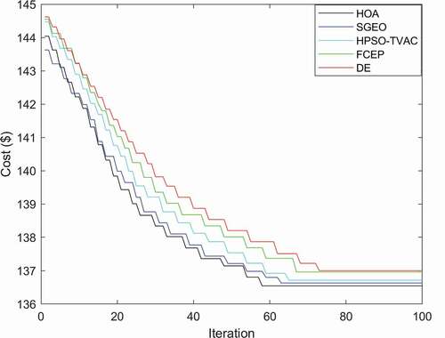
Power generation obtained from diesel generators, solar PV plants, PEVs and BESS with and without fuel constraints corresponding to best cost obtained from HOA is shown in Figure 2 and Figure 5 respectively. Fuel delivered to diesel generators corresponding to best cost obtained from HOA with fuel constraints are given in Table 1. Power generation obtained from diesel generators, solar PV plants, PEVs and BESS with and without fuel constraints corresponding to best cost obtained from SGEO is shown in Figure 3 and Figure 6 respectively. Fuel delivered to diesel generators corresponding to best cost obtained from SGEO with fuel constraints are given in Table 2. Power generation obtained from diesel generators, solar PV plants, PEVs and BESS with and without fuel constraints corresponding to best cost obtained from HPSO-TVAC is shown in Figure 4 and Figure 7 respectively. Fuel delivered to diesel generators corresponding to best cost obtained from HPSO-TVAC with fuel constraints are given in Table 3. The best, average and worst cost and average CPU time among 100 runs of solutions obtained from these four algorithms are summarized in Table 4. The cost convergence characteristics with and without fuel constraints are shown in Figure 8 and Figure 9 respectively. It has been observed from Table 4 that the cost in case of fuel constraints is more than the cost without fuel constraints. It has been also seen from Table 4 that the cost obtained from HOA is the lowest among all the four techniques. Due to page limitation detail results obtained from FCEP and DE are not given here.

Table 1. Fuel delivered (liter) to diesel generators obtained from HOA with fuel constraints

Interval	$Fd{g}_1$	$Fd{g}_2$
1 2 3 4 5 6	8.6625 2.1625 9.0671 8.5923 8.4710 9.2896	11.3375 17.8375 12.9329 16.4077 13.5290 10.7104

Table 2. Fuel delivered (liter) to diesel generators obtained from SGEO with fuel constraints

Interval	$Fd{g}_1$	$Fd{g}_2$
1 2 3 4 5 6	7.7092 7.0027 9.7082 8.5863 4.4807 9.6353	12.2908 12.9973 12.2918 16.4137 17.5193 10.3647

Table 3. Fuel delivered (liter) to diesel generators obtained from HPSO-TVAC with fuel constraints

Interval	$Fd{g}_1$	$Fd{g}_2$
1 2 3 4 5 6	8.8212 9.2395 9.2827 9.7192 6.3402 8.7186	11.1788 10.7605 12.7173 15.2808 15.6598 11.2814

Table 4. Comparison of performance

		Best price ($)	Average price ($)	Worst price ($)	CPU time (s)
With fuel constraints	HOA	137.1420	137.1524	137.1648	7.44
	SGEO	137.1875	137.1982	137.1996	8.05
	HPSO-TVAC	137.2230	137.2352	137.2487	8.38
	FCEP	137.3685	137.3769	137.3832	7.25
	DE	137.5102	137.5301	137.5437	7.47
Without fuel constraints	HOA	136.5432	136.5543	136.5677	6.78
	SGEO	136.6293	136.6389	136.6478	7.11
	HPSO-TVAC	136.7158	136.7288	136.7399	7.46
	FCEP	136.9600	136.9715	136.9802	6.39
	DE	136.9979	136.9998	137.0132	6.43

Figure 2. Power generation acquired from diesel generators, solar PV plants, PEVs and BESS considering fuel constraints using HOA.

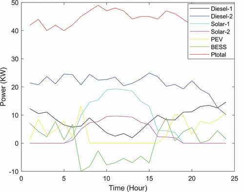
Figure 3. Power generation acquired from diesel generators, solar PV plants, PEVs and BESS considering fuel constraints using SGEO.

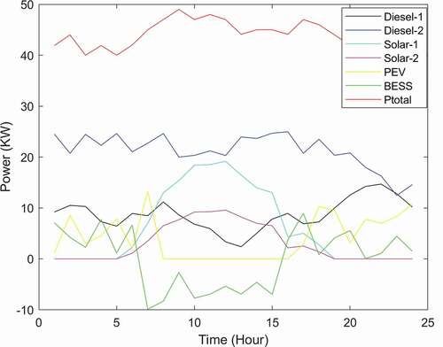
Figure 4. Power generation acquired from diesel generators, solar PV plants, PEVs and BESS considering fuel constraints using HPSO-TVAC.

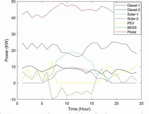
Figure 5. Power generation acquired from diesel generators, solar PV plants, PEVs and BESS without fuel constraints using HOA.

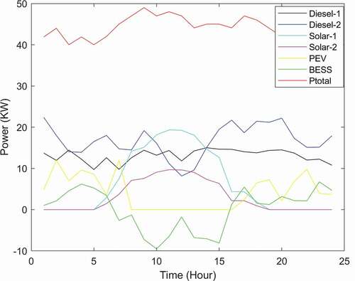
Figure 6. Power generation acquired from diesel generators, solar PV plants, PEVs and BESS without fuel constraints using SGEO.

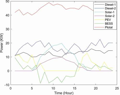
Figure 7. Power generation acquired from diesel generators, solar PV plants, PEVs and BESS without fuel constraints using HPSO-TVAC.

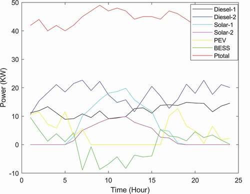
Figure 8. Cost convergence characteristics considering fuel constraints.

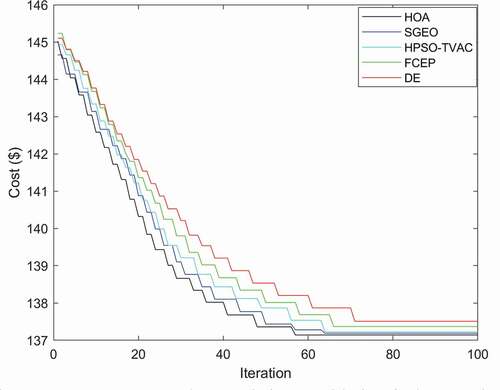
Figure 9. Cost convergence characteristics without fuel constraints.

Conclusion

In the study, HOA has been suggested to solve day in advance scheduling of isolated nanogrid with and without fuel constraints considering DSM. The suggested scheduling is performed to a nanogrid system for five neighboring homes using two diesel generators, two solar PV plants, one battery energy storage system and five plug-in electric vehicles (PEVs). Test system is also solved by using SGEO, HPSO-TVAC, FCEP and DE. It has been observed from numerical results, that the total cost with fuel constraints is more than the cost without fuel constraints. Numerical results show that fuel consumption is properly managed for satisfying constraints imposed by fuel suppliers. Though optimal scheduling is not achieved all the time, but this is generally much better than the penalty which is imposed because of fuel constraints violation. It has been also observed that the suggested HOA performs best among all the four techniques.

Nomenclature

$C_{\mathrm{T}}$: total price

$a_{di},b_{di},c_{di}$: fuel price coefficients of $i$th diesel generating unit

$\mathrm{P}d{g}_{it}$: power output of $i$th diesel generator at time $t$

$\mathrm{P}d{g}_i^{min}$,$\mathrm{P}d{g}_i^{max}$: lower and upper limits of power generation for $i$th diesel generating unit

$U{R}_{di}$, $D{R}_{di}$: ramp-up and ramp-down rate limits of the $i$th diesel generating unit

$Fd{g}_{im}$: Fuel delivered to $i$th diesel generator in interval $m$

$Fd{g}_i^{min},Fd{g}_i^{max}$: minimum and maximum fuel delivery limits of $i$th diesel generator

$F{D}_{dm}$: Total fuel delivered to all diesel generators in interval $m$

$Vd{g}_{im}$: Fuel storage of $i$th diesel generating unit in interval $m$

$Vd{g}_i^{min},Vd{g}_i^{max}$: minimum and maximum fuel storage limits of $i$th diesel generating unit

$Vd{g}_i^0$: Initial fuel storage of $i$th diesel generating unit

$\mathrm{P}p{v}_{jt}$: power output from $j$th solar PV plant at time $t$

${\mathrm{P}}_{PVrj}$: rated power output of $j$th solar PV plant

$G_t$: solar irradiation forecast at time $t$

$\mathrm{K}p{v}_j$: direct cost coefficient for the $j$th solar PV plant

$Op{v}_{jt}\left(\mathrm{P}p{v}_{jt}\right)$: reserve cost function due to overestimation of the $j$th solar PV plant at time $t$

$Up{v}_{jt}\left(\mathrm{P}p{v}_{jt}\right)$: penalty cost function due to underestimation of the $j$th solar PV plant at time $t$

$up{v}_j$, $op{v}_j$: penalty cost and reserve cost for the $j$th solar PV plant

${\mathrm{P}}_{EVlt}$: charging load of $l$th PEV at time $t$

${\mathrm{P}}_{EVl}^{min}$, ${\mathrm{P}}_{EVl}^{max}$: lower and upper charging power of $l$th PEV

$\mathrm{P}\mathrm{E}SS{C}_t$: power charge to the battery system at time $t$

$\mathrm{P}\mathrm{E}SS{D}_t$: power discharge from the battery system at time $t$

$L_{Base,t}$: predicted base load at time $t$

$D{R}_t$: percentage of predicted based load participated in DRP at time $t$

$L{s}_t$: shiftable load at time $t$

${\mathrm{N}}_d$: number of diesel generators

${\mathrm{N}}_{PV}$: number of solar PV plants

${\mathrm{N}}_{EV}$: number of PEVs

$t$, $\mathrm{T}$: time index and scheduling eon

Disclosure Statement

No potential conflict of interest was reported by the author(s).

Appendix

Table A.1: Data of diesel generators

Table

Unit$\mathrm{P}d{g}^{min}$ $\mathrm{P}d{g}^{max}$$a_d$ $b_d$ $c_d$ $U{R}_d$ $D{R}_d$ KW KW $/h $/KWh $/ KW^2h KW/h KW/h

1 0 15 2.0350 0.0602 0.000044 3 3 2 0 25 1.1825 0.0653 0.000044 5 5

Table A.2: Fuel consumption coefficients, fuel delivery limits, fuel storage limits

and initial fuel storage of diesel generators

Table

Unit ${\eta }_d$ ${\delta }_d$ ${\mu }_d$ $Fd{g}^{min}$ $Fd{g}^{max}$ $Vd{g}^{min}$ $Vd{g}^{max}$ $Vd{g}^0$ liter/h liter/MWh liter/(MW)^2h liter liter liter liter liter

1 2.00669 0.060200 0.00010033 0 10 0 20 15 2 1.33779 0.060200 0.00005017 0 20 0 40 20

Table A.3: Hourly Power demand and Temperature

Table

Hour	Power (KW)	Temperature$\left({\hspace{0.17em}}^{0}C\right)$	Hour	Power (KW)	Temperature$\left({\hspace{0.17em}}^{0}C\right)$	Hour	Power (KW)	Temperature$\left({\hspace{0.17em}}^{0}C\right)$
1 2 3 4 5 6 7 8	37 39 35 37 40 42 45 47	23 23 24 25 25 25 26 27	9 10 11 12 13 14 15 16	49 47 48 47 49 50 50 49	27 28 29 29 29 28 28 27	17 18 19 20 21 22 23 24	47 46 44 42 40 39 38 37	26 25 24 24 24 24 23 23

Table A.4. Fuel delivered

during scheduling period

Table

Interval Duration $F{D}_d$ (h) (liter)

1 4 20 2 4 20 3 4 22 4 4 25 5 4 22 6 4 20

Fig. A.1. The maximum and minimum predicted limits of solar irradiation

1) Day-ahead scheduling of isolated NG is presented.

2) Fuel constraints and ramp rate limit constraints of diesel generators are considered.

3) Demand side management is taken into consideration.

4) Horse herd optimization algorithm has been used for solving the problem.

References

- Akinyele, and D. Akinyele. 2017. Techno-economic design and performance analysis of nanogrid systems for households in energy-poor villages. Sustainable Cities and Society 34:335–57. doi:https://doi.org/10.1016/j.scs.2017.07.004.
- Aliasghari, P., B. Mohammadi-Ivatloo, Alipour, M. Alipour, M. Abapour, and K. Zare. 2018. Optimal scheduling of plug-in electric vehicles and renewable micro-grid in energy and reserve markets considering demand response program. Journal of Cleaner Production 186:293–303. doi:https://doi.org/10.1016/j.jclepro.2018.03.058.
- Alipour, M.-I., Moradi-Dalvand, and Zare. 2017. Stochastic scheduling of aggregators of plug-in electric vehicles for participation in energy and ancillary service markets. Energy 118:1168–79. doi:https://doi.org/10.1016/j.energy.2016.10.141.
- Basu. 2017. Fast Convergence Evolutionary Programming for Economic Dispatch Problems. IET Generation, Transmission & Distribution 11 (16):4009–17. doi:https://doi.org/10.1049/iet-gtd.2017.0275.
- Burmester, Rayudu, Seah, D. Burmester, R. Rayudu, W. Seah, and D. Akinyele. 2017. A review of nanogrid topologies and technologies. Renewable and Sustainable Energy Reviews 67:760–75. doi:https://doi.org/10.1016/j.rser.2016.09.073.
- Dahiru, and Tan. 2020.Optimal Sizing and Techno-economic Analysis of Grid-connected Nanogrid for Tropical Climates of the Savannah. Sustainable Cities and Society 52:1–12.
- Feng, X., Wang, Yu, Y. Wang, H. Yu, and F. Luo. 2018. A novel intelligence algorithm based on the social group optimization behaviors. IEEE Transactions on Systems, Man, and Cybernetics: Systems 48 (1):65–76. doi:https://doi.org/10.1109/TSMC.2016.2586973.
- Kumar, Tejani, Mirjalili, S. Kumar, G. G. Tejani, and S. Mirjalili. 2019. Modified symbiotic organisms search for structural optimization. Engineering with Computers 35 (4):1269–96. doi:https://doi.org/10.1007/s00366-018-0662-y.
- Kumar, Vemuri, A. B. Kumar, and S. Vemuri. 1984. Fuel resource scheduling, Part-II- contrained economic dispatch. IEEE Transactions on Power Apparatus and Systems PAS-103 (7):1549–55. doi:https://doi.org/10.1109/TPAS.1984.318624.
- Kumar, J., P. Tejani, Tejani, G. G. Alhelou, M. Premkumar, and H. H. Alhelou. 2021a. MOPGO: A new physics-based multi-objective plasma generation optimizer for solving structural optimization problems. IEEE Access 9:84982–5016. doi:https://doi.org/10.1109/ACCESS.2021.3087739.
- Kumar, S., G. G. Tejani, Pholdee, N. Pholdee, S. Bureerat, and P. Mehta. 2021b. Hybrid heat transfer search and passing vehicle search optimizer for multi-objective structural optimization. Knowledge-Based Systems 212:106556. doi:https://doi.org/10.1016/j.knosys.2020.106556.
- Kumar, S., Tejani, Pholdee, G. G. Tejani, N. Pholdee, and S. Bureerat. 2020. Improved metaheuristics through migration-based search and an acceptance probability for truss optimization. Asian Journal of Civil Engineering 21 (7):1217–37. doi:https://doi.org/10.1007/s42107-020-00271-x.
- Lee, S., J. Lee, H. Jung, Cho, J. Cho, J. Hong, S. Lee, and D. Har. 2019. Optimal power management for nanogrids based on technical information of electric appliances. Energy and Buildings 191:174–86. doi:https://doi.org/10.1016/j.enbuild.2019.03.026.
- Liang, and Liao. 2007. A fuzzy-optimization approach for generation scheduling with wind and solar energy systems. IEEE Trans. On PWRS 22 (4):1665–74.
- MiarNaeimi, Azizyan, Rashki, F. MiarNaeimi, G. Azizyan, and M. Rashki. 2021. Horse herd optimization algorithm: A nature-inspired algorithm for high-dimensional optimization problems. Knowledge-Based Systems 213 (106711):1–17. doi:https://doi.org/10.1016/j.knosys.2020.106711.
- Morsali, Kowalczy, R. Morsali, and R. Kowalczyk. 2018. Demand response based day-ahead scheduling and battery sizing in microgrid management in rural areas. IET Renewable Power Generation 12 (14):1651–58. doi:https://doi.org/10.1049/iet-rpg.2018.5429.
- Ratnaweera, Halgamuge, Watson, A. Ratnaweera, S. K. Halgamuge, and H. C. Watson. 2004. Self-organizing hierarchical particle swarm optimizer with time-varying acceleration coefficients. IEEE Transactions on Evolutionary Computation 8 (3):240–55. doi:https://doi.org/10.1109/TEVC.2004.826071.
- Shilaja, Ravi, C. Shilaja, and K. Ravi. 2017. Optimization of emission/economic dispatch using Euclidean affine flower pollination algorithm (eFPA) and binary FPA (BFPA) in solar photo voltaic generation. Renewable Energy 107:550–66. doi:https://doi.org/10.1016/j.renene.2017.02.021.
- Tejani, Kumar, and Gandomi. 2019. Multi-objective heat transfer search algorithm for truss optimization. Engineering with Computers 1–22.
- Trefny, Lee, F. Trefny, and K. Lee. 1981. Economic fuel dispatch. IEEE Transactions on Power Apparatus and Systems PAS-100 (7):3468–77. doi:https://doi.org/10.1109/TPAS.1981.316690.
- Vemuri, K., E. Hackett, and Lugtu. 1984. Fuel resource scheduling, Part-I- overview of an energy management problem. IEEE Trans. Power Apparatus and Systems, PAS-103 7:1542–48.