A Hybrid Machine Learning Model for Credit Approval

ABSTRACT

Incorrect decision-making in financial institutions is very likely to cause financial crises. In recent years, many studies have demonstrated that artificial intelligence techniques can be used as alternative methods for credit scoring. Previous studies showed that prediction models built using hybrid approaches perform better than single approaches. In addition, feature selection or instance selection techniques should be incorporated into building prediction models to improve the prediction performance. In this study, we integrate feature selection, instance selection, and decision tree techniques to propose a new approach to predicting credit approval. Experimental results obtained using the survey data show that our proposed approach is superior to the other five traditional machine learning approaches in the measures. In addition, our approach has a lower cost effect than the traditional five methods. That is, the proposed approach generates fewer costs, such as money loss, than the traditional five approaches.

Introduction

Credit-risk evaluation decisions are important for the financial institutions involved due to the high level of risk associated with wrong decisions. The ability to accurately predict credit failure is a very important issue in financial decision-making. Incorrect decision-making in financial institutions is very likely to cause financial crises (Tsai 2014). The purpose of credit scoring is to classify the applicants into two types: applicants with good credit and applicants with bad credit. Even a 1% improvement in the accuracy of the credit scoring of applicants with bad credit can greatly decrease the losses of financial institutions (Hand and Henley 1997).

In recent years, many studies have demonstrated that artificial intelligence (AI) techniques can be used as alternative methods for credit scoring, such as artificial neural networks (ANN) (Guotai, Abedin, and Moula 2017; Tsai 2014; Wang et al. 2011), decision trees (DT) (Tsai 2014; Wang et al. 2011), and support vector machines (SVM) (Chen and Li 2014; Zhong et al. 2014). Previous studies showed that prediction models built using hybrid approaches, such as classifiers with clustering, perform better than single approaches (classifiers only) (Hsieh 2005; Luo, Cheng, and Hsieh 2009; Ping and Yongheng 2011). Moreover, some previous studies revealed that feature selection (Catal and Diri 2009; Lee 2009; Saeys, Inza, and Larrañaga 2007; Tsai 2009; Tsai and Hsiao 2010) or instance selection (Sun and Li 2011; Tsai and Cheng 2012) should be incorporated into building prediction models to improve prediction performance.

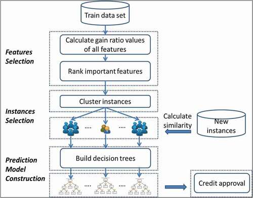
In this study, we propose a new approach, integrating feature selection, instance selection, and classifier to build a prediction model for credit approval. The proposed framework is shown in Figure 1. Its process is described as follows. First, a measure (gain ratio) is used for feature selection. Second, a clustering method, expectation maximization (EM), is applied to cluster training dataset into k clusters in advance. Finally, a classification method, called the C4.5 algorithm, is used to build k decision tree classifiers for k clusters of instances.

Figure 1. The proposed framework.

In the experiment, we use measures named precision, true positive rate (TPR), accuracy, and F₁ to evaluate the performance difference between the proposed approach and five traditional machine learning approaches, DT (decision tree), MLP (multiple-layer perceptron), NB (naive Bayes classifiers), RF (random forest), and SVM (support vector machine). In addition, we also use the cost-effect to evaluate the cost-effectiveness analysis (CEA) of the proposed approach and the five traditional machine learning approaches (DT, MLP, NB, RF, and SVM).

The rest of this paper is organized as follows. Section 2 reviews related work. The proposed clustering-based decision tree is illustrated in Section 3. The evaluation criteria are illustrated in Section 4. Case studies based on real data are used to demonstrate the experimental results in Section 5. Section 6 discusses the conclusions and offers suggestions for future work.

Related Work

Decision Tree Related Works

Classification is an important problem in the field of data mining. In classification, we are given a set of example records, called the training data set, with each record consisting of several attributes. One of the categorical attributes, called the class label, indicates the class to which each record belongs. The objective of classification is to utilize the training data set to build a model of the class label such that it can be used to classify new data whose class labels are unknown.

Many types of models have been built for classification, such as neural networks, statistical models, genetic models, and decision tree models (Han, Kamber, and Pei 2006). Classification trees, also called decision trees, are especially attractive in a data mining environment for several reasons (Breiman et al. 1984). First, due to their intuitive representation, the resulting classification model is easy for human beings to assimilate (Mehta, Agrawal, and Rissanen 1996). Second, decision trees do not require any parameter settings from the user and thus are especially suited for exploratory knowledge discovery. Third, decision trees can be constructed relatively quickly compared to other methods (Shafer, Agrawal, and Mehta 1996). Finally, the accuracy of decision trees is comparable or superior to that of other classification models (Lim, Loh, and Shih 1998).

Related to decision tree classifiers, Quinlan (1986) proposed a decision tree algorithm known as Iterative Dichotomiser 3 (ID3). Later, Quinlan (1987) proposed C4.5 (a successor of ID3), which became a benchmark work to which newer supervised learning algorithms are often compared. Breiman et al. (1984) proposed the classification and regression tree (CART) algorithm, which describes the generation of binary decision trees. Other algorithms for decision tree induction include SLIQ (Mehta, Agrawal, and Rissanen 1996), SPRINT (Shafer, Agrawal, and Mehta 1996), BOAT (Gehrke et al. 1999) and so on. The efficiency of existing decision tree algorithms, such as ID3, C4.5, and CART, has been well established for relatively small data sets. The SPRINT and SLIQ algorithms can both handle categorical and continuous valued attributes and are also suitable for very large training sets. The BOAT algorithm can be used for incremental updates. That is, BOAT can take new insertions and deletions for the training data and update the decision tree to reflect these changes (Han, Kamber, and Pei 2006).

An attribute selection measure is a heuristic for selecting the splitting criterion that separates a given data partition of class-labeled training tuples into individual classes. The presence of redundant attributes does not adversely affect the accuracy of decision trees. An attribute is redundant if it is strongly correlated with another attribute in the data. One of the two redundant attributes is not used for splitting once the other attribute has been chosen. However, if the data set contains many irrelevant attributes, i.e., attributes that are not useful for the classification task, then some of these may be accidentally chosen during the tree-growing process, resulting in a decision tree that is larger than necessary (Tan, Steinbach, and Kumar 2006).

Clustering methods are used to improve the accuracy of decision trees by eliminating the irrelevant attributes. Pushpalatha and Rajalakshmi (2018) analyzed the importance of attribute selection techniques in a credit approval dataset. According to their study, logistic regression with the CFSSubsetEval attribute selection method yields better performance when compared to other techniques. Pristyanto, Adi, and Sunyoto (2019) proposed a proper feature selection model for increasing the accuracy of specific classifier models by comparing several existing feature selection models and some classifiers.

The related studies about the development or improvement for the classification techniques are of abundance. Due to space limitation, the researches of Ngai, Xiu, and Chau (2009) and Ngai et al. (2011) provide the literature review for the classification topic.

Clustering Related Works

The k-means (KM) approach has been widely used in pattern recognition problems. Several variations and improvements to the original algorithm have been made. MacQueen’s (1967) k-means algorithm is widely used because of its simplicity. This algorithm has been shown to converge to a local minimum (Selim and Ismail 1984). Elsewhere, it has been shown that there is no guarantee of optimal clustering, since the convergence depends on the initial seeds selected (Looney 2002). The k-means algorithm, however, is not considered to be the best choice for clustering due to its poor time performance and other requirements. It typically requires that clusters should be spherical, that the data should be free of noise and that its operation should be properly initialized (Estivill-Castro and Yang 2004).

Expectation maximization (EM) (Dempster, Laird, and Rubin 1977) is an improved version of the k-means algorithm, with better performance. It is a statistical technique for maximum likelihood estimation using mixed models. The EM algorithm is the most frequently used technique for estimating class conditional probability density functions (PDF) (Abd-Almageed, El-Osery, and Smith 2003).

EM clusters data in a manner different than in the k-means method. Unlike distance-based or hard membership algorithms (such as k-Means), EM is known to be an appropriate optimization algorithm for constructing proper statistical models of data (Bradley and Fayyad 1998). However, convergence to a local rather than the global optima is a problem arising due to its iterative nature. This means that the method is sensitive to the initial conditions, and thus not robust. To overcome the initialization problem, several methods for determining ‘good’ initial parameters for EM have been suggested, mainly based on sub-sampling, voting, and two-stage clustering (Meila and Heckerman 1998).

EM aims at finding clusters such that the maximum likelihood of each cluster’s parameters is obtained. EM starts with an initial estimate for the missing variables and iterates to find the maximum likelihood (ML) for these variables. Maximum likelihood methods estimate the parameters by values that maximize the sample’s probability for an event. EM is typically used with mixture models. The goal of the EM algorithm is to maximize the overall probability or likelihood of the data, given the (final) clusters. Unlike the classic implementation of k-means clustering, the general EM algorithm can be applied to both continuous and categorical variables (Bradley, Fayyad, and Reina 1998).

The related research about the development or improvement for the classification techniques is abundant. Due to space limitation, the studies of Levin (2015), Reddy and Ussenaiah (2012), and Xu and Tian (2015) provide the literature review for the clustering topic.

Credit Scoring

The purpose of credit scoring is to classify the applicants into two types: applicants with good credit and applicants with bad credit. Applicants with good credit are very likely to repay their financial obligation. Those with bad credit have a high possibility of defaulting. The accuracy of credit scoring is critical to financial institutions’ profitability. Even a 1% improvement in the accuracy of credit scoring of applicants with bad credit can greatly decrease the losses of financial institutions (Hand and Henley 1997).

Credit scoring was originally evaluated subjectively according to personal experiences. However, with the tremendous increase of applicants, it is impossible to conduct the work manually. Statistical techniques and artificial intelligence (AI) techniques, which are the two major categories of automatic credit scoring techniques, have been investigated in prior studies (Huang et al. 2004). In addition, Huang et al. (2004) found that AI techniques are superior to statistical techniques in dealing with credit scoring problems, especially for nonlinear pattern classification. Muniyandi, Rajeswari, and Rajaram (2012) proposed an anomaly detection method using “k-Means + C4.5,” a method to cascade k-means clustering and C4.5 decision tree methods for classifying anomalous and normal activities in a computer network.

In recent years, many studies have demonstrated that AI techniques, such as artificial neural networks (ANN) (Chang and Yeh 2012; Hájek 2011; Tsai 2014; Wang et al. 2011), stochastic gradient boosting (Orlova 2021), decision trees (DT) (Inyaem and Chuaytem 2020; Tsai 2014; Wang et al. 2011), ensemble model (Nalić, Martinović, and Žagar 2020; Zhang et al. 2021), and support vector machines (SVM) (Chen and Li 2014; Kim and Ahn 2012; Tsai 2014; Wang et al. 2011; Wang and Ma 2012; Yeh, Lin, and Hsu 2012; Zhong et al. 2014) can be used as alternative methods for credit scoring. For completely understanding the previous studies, the survey of Dastile, Celik, and Potsane (2020) proffers the literature review with respect to this issue.

Table 1 compares hybrid learning models related to credit rating techniques and evaluation methods. In the related works, previous hybrid models are generally compared with single machine learning techniques to make the final conclusion.

Table 1. Comparison of works

Work	Techniques	Evaluation
Chen and Li (2010)	Feature selection (FS) + Classifiers (SVM)	Accuracy and error rates
Hsieh (2005)	Clustering (KM) + Classification (ANN)	Accuracy and error rates
Hsieh and Hung (2010)	Clustering (KM) + Classification (ANN)	Association rules for bad credit status
Huang, Chen, and Wang (2007)	Feature selection (FS) + Classifiers (SVM)	Accuracy rates
Huysmans et al. (2006)	Classification + Clustering (Self-Organizing Map, SOM)	Accuracy rates
Koutanaei, Sajedi, and Khanbabaei (2015)	Feature selection (FS) + Classifiers	Accuracy and error rates
Lee et al. (2002)	Classification + Classification	Accuracy and error rates
Luo, Cheng, and Hsieh (2009)	Classifiers	Accuracy rates
Malhotra and Malhotra (2002)	Classification + Classification	Accuracy rates
Ping and Yongheng (2011)	Feature selection (FS) + Classifiers (SVM)	Accuracy rates
Zhao et al. (2015)	Instance selection (IS) + Classifiers (Multilayer perceptron, MLP)	Error rates
Pristyanto, Adi, and Sunyoto (2019)	Feature selection (FS) + Classifiers	Accuracy rates

From the above discussion, we know that (1) hybrid data mining approaches are popular for building prediction models (classifiers); (2) feature selection techniques are integrated for building classifiers; and (3) instance selection techniques are integrated for building classifiers. However, feature selection and instance selection techniques are not integrated together for building prediction models (classifiers).

In general, we comprehend that a data-driven approach is sensitive to the distribution of datasets. Hence, there is no any best machine learning algorithm to outperform other algorithms. Researchers attempt to use different data-preprocessing strategies to remedy the problem. The first technique, feature selection, is to reckon the level of feature representativeness for distinguishing higher discriminative features. The second, instance selection, is to reduce the size of datasets and filter out noises or outliers from datasets. However, the past studies only employ one technique to develop their research models in the field of credit scoring. Therefore, this study adopts both respective advantages to strengthen the power of data-driven approaches. The idea is similar to the mixing and matching strategy of COVID-19 vaccines. AstraZeneca and Moderna own their different ways to produce antibodies for COVID-19; therefore, governments adopt both to comprehensively ensure national health. The strategy of this study is the same as the above argument to assure that we could discover the best rules/patterns from any type of datasets by our proposed model.

In addition, the cost-effect criterion has not been considered in previous studies to evaluate the performance of prediction models. Therefore, we attempt to integrate feature selection, instance selection, and decision tree techniques to propose a new approach to predicting credit approval.

The Proposed Approach

In this study, we first use gain-ratio to determine clustering attributes (feature selection). After that, we apply the EM clustering technique to cluster the training data into k clusters (instance selection). For each cluster of the dataset, we use the C4.5 decision tree algorithm to build a decision tree classifier (prediction model construction). Finally, there are k C4.5 decision trees generated from k clusters of the dataset. That is, each cluster of the dataset is used to build a C4.5 decision tree. When predicting the class labels of the unseen data, the cluster IDs of the unseen data are first determined by the EM clustering algorithm (such as cluster ID = 2). The specific cluster’s C4.5 decision tree (cluster ID = 2) is then used to predict the class labels of the unseen data.

Decision Tree

Quinlan (1986) proposed a decision tree algorithm, related decision tree classifiers known as ID3. Later, Quinlan (1987) proposed C4.5 (a successor of ID3), which became a benchmark work to which newer supervised learning algorithms are often compared. In this section, we illustrate two popular measures, information gain, and gain ratio, used to select the splitting attribute.

Information Gain

ID3 uses information gain as its attribute selection measure. Let D, the partition, be a training set of class-labeled tuples. Suppose the class label attribute has m distinct values defining m distinct classes, C_i (for i = 1, 2, …, m). Let C_i, _D be the set of tuples of class C_i in D. Let |D| and |C_i, _D| denote the number of tuples in D and C_i, _D, respectively. Let node N represent the tuples of partition D. The attribute with the highest information gain is chosen as the splitting attribute for node N. This attribute minimizes the information needed to classify the tuples in the resulting partitions, reflecting the “impurity” in these partitions. The expected information needed to classify a tuple in D is given by

(1) $Info(D)=-\sum _{i=1}^m{p}_i{log}_2(p_i)$(1)

where p_i is the probability that an arbitrary tuple in D belongs to class C_i and is estimated by |C_i, _D|/|D|. A log function to base 2 is used, because the information is encoded in bits. Info(D) is just the average amount of information needed to identify the class label of a tuple in D. Info(D) is also known as the entropy of D.

Suppose we want to partition the tuples in D on some attribute A having v distinct values, {a₁, a₂, …, a_v}, as observed from the training data. Attribute A can be used to split D into v partitions or subsets, {D₁, D₂, …, D_v}, where D_j contains those tuples in D that have outcome a_j of A. These partitions correspond to the branches grown from node N. After partitioning, it is quite likely that the partitions will be impure (e.g., may contain a collection of tuples from different classes rather than from a single class). How much more information do we still need (after the partitioning) in order to arrive at an exact classification? The amount is measured by

(2) $Inf{o}_A(D)=\sum _{j=1}^v\frac{\left|D_j\right|}{\left|D\right|}\times Info(D_j)$(2)

where $\frac{\left|D_j\right|}{\left|D\right|}$ is the weight of the jth partition; $Inf{o}_A(D)$is the expected information required to classify a tuple from D based on the portioning by A. The smaller the amount of expected information required, the greater the purity of the partitions.

Information gain is defined as the difference between the original information requirement (i.e., based on just the proportion of classes) and the new requirement (i.e., obtained after portioning based on attribute A). That is

Gain(A) = Info(D) – Info_A(D). (3)

Gain(A) tells us how much would be gained by branching based on A. If attribute A holds the highest information gain, Gain(A), it is chosen as the splitting attribute at node N. That is, we partition based on attribute A for the “best classification,” so as to minimize the amount of information still required to finish classifying the tuples (i.e., minimum Info_A(D)).

Gain Ratio

The information gain measure is biased toward tests with many outcomes. That is, it prefers to select attributes having a large number of values, such as customer_ID. The information required to classify data set D based on this partition would be Info_{customer_ID}(D) = 0. Therefore, the information gained by partitioning based on this attribute is maximal. However, such a partitioning is useless for classification.

C4.5, a successor of ID3, uses an extension to the information gain known as the gain ratio, as an attempt to overcome this bias. A kind of normalization is applied to the information gain using a “split information” value defined analogously with Info(D) as

(4) $SplitInf{o}_A(D)=-\sum _{j=1}^v\frac{\left|D_j\right|}{\left|D\right|}\times {log}_2(\frac{\left|D_j\right|}{\left|D\right|})$(4)

This value represents the potential information generated by splitting the training data set, D, into v partitions, corresponding to the v outcomes of a test on attribute A. Note that, for each outcome, the number of tuples having that outcome with respect to the total number of tuples in D is considered. This method differs from information gain, which measures the information with respect to classification that is acquired based on the same partitioning. The attribute with the maximum gain ratio is selected to be the splitting attribute. The gain ratio is defined as

(5) $GainRatio(A)=\frac{Gain(A)}{SplitInf{o}_A(D)}$(5)

The Expectation Maximization (EM) Clustering Method

Clustering analysis is an important activity for dealing with large amounts of data. Automated clustering can be used to identify dense and sparse regions in an object space and, therefore, discover overall distribution patterns and interesting correlations among the data attributes. Therefore, clustering is also called data segmentation in some applications, because clustering partitions large data sets into groups according to their similarity.

The most well-known and commonly used partitioning methods are k-means, expectation maximization (EM), and their variations. The k-means algorithm takes the input parameter, k, and partitions a set of n objects into k clusters so that the resulting intra-cluster similarity is high but the inter-cluster similarity is low. The k-means algorithm is a popular clustering algorithm that requires a huge initial set to start the clustering. This is an unsupervised clustering method that does not guarantee convergence. EM is an improvement of the k-means algorithm that offers better performance. It is a statistical technique for maximum likelihood estimation using mixture models.

The EM algorithm is an iterative statistical technique for maximum likelihood estimation in settings with incomplete data. Given a model of data generation and data with some missing values, EM locally maximizes the likelihood of the model parameters and estimates the missing values. The steps for our implementation of EM are described below. Initially, we guess the mean and standard deviation. Then, the EM algorithm searches for an ML hypothesis through the following iterative scheme (Nasser, Alkhaldi, and Vert 2006).

1. Step 1 Initialization: initialize the hypothesis θ⁰ = (μ⁰₁, μ⁰₂, …, μ⁰_k)

(6) ${\theta }_k^0={\mu }_k^0$(6)

where k is the current number of Gaussians; θ⁰ is the estimate at the 0th iteration; μ is the mean.

1. Step 2 Expectation step: estimate the expected values of the hidden variables z_ij (mean and standard deviation) using the current hypothesis θ^t = (μ^t₁, μ^t₂, …, μ^t_k)

(7) $E(z_{ik})=\frac{exp[-\frac{{(x_i-{\mu }_k^t)}^2}{2{\sigma }^2}]}{\sum _{j=1}^{K}exp[-\frac{{(x_i-{\mu }_j^t)}^2}{2{\sigma }^2}]}$(7)

where t is the number of iterations; E(z_ik) is the expected value for the hidden variables (namely mean and standard deviation); k is the dimension; μ is the mean; σ is the standard deviation.

1. Step 3 Maximization step: provide a new estimate of the parameters.

(8) ${\mu }_k^{t+1}=\frac{\sum _{i=1}^{n}E(z_{ik})x_i}{\sum _{i=1}^{n}E(z_{ik})}$(8)

1. Step 4 Convergence step: if ||θ^t+1− θ^t|| < e, stop (finish iteration); otherwise, go to step 2.

The Proposed Framework

The proposed framework is shown in Figure 1. The proposed framework involves three phases. We introduce a clustering-based decision tree (CBDT) algorithm to implement the proposed framework as shown in Figure 2. In the first phase, the measure (gain ratio) is used to evaluate features (attributes) for feature selection. We rank important features according to the measure (gain ratio). In the second phase, the clustering approach (EM) is used to cluster instances into different clusters for instance selection. In the third phase, the C4.5 decision tree method is employed to build prediction models (decision trees) for each cluster determined in the previous phase for prediction model construction.

1. Phase 1. Determine the clustering attributes:

Figure 2. The CBDT algorithm.

For training data, we first calculate Gain-Ratio values of all attributes and then select clustering attributes to cluster the data into k clusters in the second phase.

1. Phase 2. Cluster the training data into k clusters by using the EM clustering method (see Figure 3):

Figure 3. EM_Clustering Subroutine.

The EM algorithm is used to cluster the data into k clusters based on the clustering attributes generated from Phase 1.

1. Phase 3. Build decision trees for each cluster’s training data (see Figure 4):

Figure 4. Generate_Decision_Tree Subroutine.

After k clusters of training data are generated in Phase 2, we start to build decision trees for each cluster. Since we have clustered k clusters in Phase 2, we will build k decision trees. Note that, each decision tree is built from different clusters of training data.

The EM_Clustering subroutine is summarized in Figure 3. The steps for our implementation of EM_Clustering are as follows. The EM_Clustering subroutine includes two parameters, D and clustering_attributes. We refer to D as a data partition. Initially, a complete set of training records describes the records. The clustering_attributes specify the attribute that “best” discriminates the given records according to class.

The EM_Clustering subroutine starts with an initial guess for the mean and standard deviation from the Data partition (D) according to clustering_attributes (step 1). The recursive clustering stops only when ||θ^t+1− θ^t|| < e (step 5). Otherwise, the recursive clustering repeats the Expectation step and Maximization step. The expected values of the hidden variables (mean and standard deviation) in the expectation step are estimated using the current hypothesis (step 3). The maximization step provides a new estimate of the parameters (step 4).

The decision tree algorithm, C4.5, adopts a greedy approach in which decision trees are constructed in a top-down recursive divide-and-conquer manner. Most algorithms for decision tree induction also follow such a top-down approach, which starts with a set of records and their associated class labels. The training set is recursively partitioned into smaller subsets as the tree is being built. A basic decision tree algorithm is summarized in Figure 4. It is quite straightforward. The strategy is as follows.

The Generate_Decision_Tree subroutine has three parameters: D, attribute_list, and Attribute_selection_method. We refer to D as a data partition. Initially, it is the complete set of training records describing the records. Attribute_selection_method specifies a heuristic procedure for selecting the attribute that “best” discriminates between the given records according to class.

The tree starts as a single node, N, which represents the training records in D (step 1). The partition of class-labeled training records at node N is the set of records following a path from the root of the tree to node N. The set is sometimes referred to in the literature as the family of records at node N. The recursive partitioning process stops only when any one of the following terminating conditions is true: (1) if the records in D are all of the same class, then node N becomes a leaf and is labeled with that class (steps 2 and 3); (2) there are no remaining attributes on which the records may be further portioned (step 4). In this case, majority voting is employed (step 5). This involves converting node N into a leaf and labeling it with the most common class in D; (3) there are no records for a given branch, that is, a partition D_j is empty (step 12). In this case, a leaf is created with the majority class in D (step 13).

Step 6 utilizes the Attribute_selection_method to determine the splitting criterion. The splitting criterion tells us which attribute to test at node N by determining the “best” way to separate or partition the records in D into individual classes. Step 7 labels node N with the splitting criterion. A branch is grown from node N for each outcome of the splitting criterion. The records in D are partitioned accordingly (steps 10 to 11).

Experimental Results

We conducted several experiments to evaluate the proposed approach. Three credit datasets (German credit data, Australian credit approval, and credit-approval), which were obtained from the UCI machine learning repository (Dua and Graf, 2019), are used for evaluating the performance of the proposed approach.

For each run of cross-validation, we first apply the C4.5 decision tree algorithm to build a single decision tree for the baseline model. In addition, there are several machine learning methods used to compare the proposed CBDT approach. These methods are MLP, NB, RF, and SVM. The five methods, including DT, MLP, NB, RF, and SVM, were implemented to build prediction models by using Python language. The two hybrid approaches, feature selection and instance selection (EM method), were implemented by using SQL Server BI.

Furthermore, we also investigate if two hybrid approaches (feature selection and instance selection) could improve the prediction performance of the other three methods (MLP, NB, and SVM). Since RF (Random Forest) is an ensemble method, we would not integrate two hybrid approaches (feature selection and instance selection) into RF method. Therefore, we would generate three new methods (CBMLP, CBNB, and CBSVM) from three methods (MLP, NB, and SVM) integrated with two hybrid approaches (feature selection and instance selection).

Comparisons of six approaches are listed in Table 2. The parameter settings used to construct the prediction models (CBDT) are shown in Table 3.

Table 2. Comparison of the six approaches

Approaches	Features selection	Instances selection	Prediction model
DT	None	None	C4.5
MLP	None	None	Multiple Layer perceptron
NB	None	None	Naive Bayes classifier
RF	None	None	Random Forest
SVM	None	None	Support Vector Machine
CBDT (this study)	Gain-ratio	EM	C4.5

Table 3. Parameter settings of the proposed CBDT model

Aim	Model	Parameters
Clustering	EM	Cluster_Count = 2
		Clustering_Method = 1 (EM)
		Mininmum_support = default
		Modeling_Cardinality = default
		Stoping_Tolerance = default
Prediction	C4.5	Complexity_Penalty = default
		Mininmum_support = default
		Score_Method = default
		Split_Method = default

Evaluation Criteria

The confusion matrix is a useful tool for analyzing how well the classifier can recognize tuples of different classes. A confusion matrix for two classes is shown as Table 4. Given two classes, we can talk in terms of positive tuples versus negative tuples. True positives refer to the positive tuples that were correctly labeled by the classifier, while true negatives are the negative tuples that were correctly labeled by the classifier. False positives are the negative tuples that were incorrectly labeled. Similarly, false negatives are the positive tuples that were incorrectly labeled.

Table 4. Confusion matrix for positive and negative tuples

	Predicted Class
Actual Class		C1 (P)	C2 (N)
	C1 (P)	True Positives (TP)	False Negatives (FN)
	C2 (N)	False Positives (FP)	True Negatives (TN)

TP: the number of true positives; FP: the number of false positives;

TN: the number of true negatives; FN: the number of false negatives.

The true positive rate (TPR) is the proportion of positive tuples that are correctly identified. The accuracy of a classifier on a given test dataset is indicated by the percentage of test dataset tuples that are correctly classified by the classifier. Recall, referred to as the true positive rate (TPR), measures the fraction of positive examples correctly predicted by the classifier. Precision determines the fraction of records, actually turning out to be positive in the group that the classifier has declared as a positive class. Recall (TPR) and Precision are summarized into another metric known as the F₁ measure. These measures are defined as follows (Tan, Steinbach, and Kumar 2006):

(9) $Recall=TPR=\frac{TP}{TP+FN}$(9)

(10) $Precision=\frac{TP}{TP+FP}$(10)

(11) $Accuracy=\frac{(TP+TN)}{(TP+FP+FN+TN)}$(11)

(12) $F_1=\frac{2\times Recall\times Precision}{Recall+Precision}$(12)

In this study, we also apply cost-effectiveness analysis (CEA), which compares the relative costs and outcomes (effects) to evaluate the performance. A cost matrix is shown in Table 5. The cost effect measure is defined as follows.

(13) $CostEffect=\frac{(TP\times TPC+FP\times FPC+FN\times FNC+TN\times TNC)}{(TP+FP+FN+TN)}$(13)

Table 5. Cost matrix

		Predicted Class
		P	N
Actual Class	P	TPC	FNC
	N	FPC	TNC

TPC: the cost of true positives; FPC: the cost of false positives;

TNC: the cost of true negatives; FNC: the cost of false negatives.

In the experiment, we use the measures named Precision, TPR, F₁, and Accuracy to evaluate the performance differences between the proposed CBDT approach and the other five approaches listed in Table 2. Moreover, we also apply cost-effectiveness analysis (CEA) in this study. A cost matrix (see Table 6) is provided on the Statlog (German credit data) dataset website. The rows represent the actual classification and the columns represent the predicted classification. It is worse to classify a customer as good when they are bad (cost = 5) than it is to classify a customer as bad when they are good (cost = 1).

Table 6. Cost matrix for credit approval

		Predict
		P(Good)	N(Bad)
Actual	P(Good)	0	1
	N(Bad)	5	0

Statlog (German Credit Data) Dataset

There are 1000 instances in the German-credit-data dataset. This file has been edited, and several indicator variables are added to make it suitable for algorithms that cannot cope with categorical variables. Several attributes that are ordered categorically (such as attribute 17) have been coded as integers.

Firstly, we compare the proposed CBDT approach with the other five methods (DT, MLP, NB, RF, and SVM) in prediction performance. The average experimental results compared with the other five methods for 3-fold cross-validation are shown in Table 7. From Table 7, it can be seen that the proposed CBDT approach with F₁ (0.92) has higher prediction performance than the other five methods. Besides, the proposed CBDT approach with Accuracy (0.89) has higher prediction performance than the other five methods. Please note that the proposed CBDT approach with CostEffect (0.28) has lower cost effect than the other five methods. It is very important to note that the proposed CBDT approach generates the lowest costs (such as money loss) among the six approaches.

Table 7. The average experiment results compared with the other 5 methods

Method	Precision	TPR/Recall	F1	Accuracy	CostEffect
CBDT	0.93	0.91	0.92	0.89	0.28
DT	0.92	0.84	0.88	0.84	0.35
MLP	0.74	0.96	0.84	0.73	1.24
NB	0.84	0.80	0.82	0.75	0.69
RF	0.79	0.94	0.86	0.78	0.91
SVM	0.85	0.94	0.89	0.83	0.67

Secondly, we investigate if two hybrid approaches (feature selection and instance selection) could improve the prediction performance of the other three methods (MLP, NB and SVM). The average experimental results compared with the three new methods (CBMLP, CBNB, and CBSVM) are shown in Table 8. From Table 8, it can be seen that the new method (CBSVM) which integrated with hybrid approaches (feature selection and instance selection) outperform than the original method (SVM) in measures (Precision, TPR, F₁, Accuracy, and CostEffect).

Table 8. The average experiment results of the new three methods

Method	Precision	TPR	F1	Accuracy	CostEffect
CBMLP (MLP)	0.74 (0.74)	0.97 (0.96)	0.84 (0.84)	0.73 (0.73)	1.24 (1.24)
CBNB (NB)	0.80 (0.84)	0.39 (0.80)	0.53 (0.82)	0.50 (0.75)	0.78 (0.69)
CBSVM (SVM)	0.86 (0.85)	0.96 (0.94)	0.91 (0.89)	0.86 (0.83)	0.58 (0.67)

Finally, we compare the proposed CBDT approach with the new methods (CBMLP, CBNB, and CBSVM) in prediction performance. The average experimental results compared with the three new methods (CBMLP, CBNB, and CBSVM) of the Statlog (German credit data) dataset for 3-fold cross-validation are shown in Table 9. From Table 9, it can be seen that the proposed CBDT approach with F₁ (0.92) still has higher prediction performance than the other five methods. Besides, the proposed CBDT approach with Accuracy (0.89) still has higher prediction performance than the other three methods. Please note that the proposed CBDT approach with CostEffect (0.28) still has lower cost effect than the other three methods.

Table 9. The average experiment results compared with the other three methods

Method	Precision	TPR	F1	Accuracy	CostEffect
CBDT	0.93	0.91	0.92	0.89	0.28
CBMLP	0.74	0.97	0.84	0.73	1.24
CBNB	0.80	0.39	0.53	0.50	0.78
CBSVM	0.86	0.96	0.91	0.86	0.58

Statlog (Australian Credit Approval) Dataset

There are 690 instances in the Australian-credit-approval dataset. This file concerns credit card applications. All attribute names and values have been changed to meaningless symbols to protect the confidentiality of the data. This dataset is interesting because there is a good mix of attributes – continuous, nominal with small numbers of values, and nominal with larger numbers of values. That is. All attributes have been coded as integers.

Firstly, we compare the proposed CBDT approach with the other five methods (DT, MLP, NB, RF, and SVM) in prediction performance. The average experimental results compared with the other five methods for 3-fold cross-validation are shown in Table 10. From Table 10, it can be seen that the proposed CBDT approach with F₁ (0.92) has higher prediction performance than the other five methods. Besides, the proposed CBDT approach with Accuracy (0.93) has higher prediction performance than the other five methods. Please note that the proposed CBDT approach with CostEffect (0.20) has lower cost effect than the other five methods. It is very important to note that the proposed CBDT approach generates the lowest costs (such as money loss) among the six approaches.

Table 10. The average experiment results compared with the other five methods

Method	Precision	TPR/Recall	F1	Accuracy	CostEffect
CBDT	0.92	0.92	0.92	0.93	0.20
DT	0.81	0.90	0.85	0.85	0.56
MLP	0.76	0.51	0.46	0.60	1.18
NB	0.82	0.62	0.70	0.78	0.46
RF	0.76	0.87	0.80	0.79	0.83
SVM	0.64	0.67	0.57	0.71	0.87

Secondly, we investigate if two hybrid approaches (feature selection and instance selection) could improve the prediction performance of the other three methods (MLP, NB, and SVM). The average experimental results compared with the three new methods (CBMLP, CBNB, and CBSVM) are shown in Table 11. From Table 11, it can be seen that the new methods (CBSVM) which integrated with hybrid approaches (feature selection and instance selection) outperforms than the original method (SVM) in measures (Precision, TPR, F₁, Accuracy, and CostEffect). Besides, the new methods (CBNB) which integrated with hybrid approaches (features selection and instances selection) slightly outperforms than the original method (NB) in measures (Precision, F₁, and CostEffect).

Table 11. The average experiment results of the new three methods

Method	Precision	TPR	F1	Accuracy	CostEffect
CBMLP (MLP)	0.68 (0.76)	0.93 (0.51)	0.78 (0.46)	0.78 (0.60)	0.99 (1.18)
CBNB (NB)	0.85 (0.82)	0.61 (0.62)	0.71 (0.70)	0.78 (0.78)	0.41 (0.46)
CBSVM (SVM)	0.92 (0.64)	0.96 (0.67)	0.94 (0.57)	0.94 (0.71)	0.22 (0.87)

Finally, we compare the proposed CBDT approach with the new methods (CBMLP, CBNB, and CBSVM) in prediction performance. The average experimental results compared with the three new methods (CBMLP, CBNB, and CBSVM) of the Statlog (Australian credit approval) dataset for 3-fold cross-validation are shown in Table 12. From Table 12, it can be seen that the CBSVM approach with F₁ (0.94) has higher prediction performance than the other five methods. Besides, the CBSVM approach with Accuracy (0.94) has higher prediction performance than the other three methods. Please note that the CBSVM approach slightly outperforms than the proposed CBDT approach. However, the proposed CBDT approach with CostEffect (0.20) still has lower cost effect than the other three methods.

Table 12. The average experiment results compared with the other three methods

Method	Precision	TPR	F1	Accuracy	CostEffect
CBDT	0.92	0.92	0.92	0.93	0.20
CBMLP	0.68	0.93	0.78	0.78	0.99
CBNB	0.85	0.61	0.71	0.78	0.41
CBSVM	0.92	0.96	0.94	0.94	0.22

Credit-approval Dataset

There are 690 instances in the credit-approval dataset. The data set information are shown as follows. This file concerns credit card applications. All attribute names and values have been changed into meaningless symbols to protect the confidentiality of the data. This dataset is interesting because there is a good mix of attributes – continuous, nominal with small numbers of values, and nominal with larger numbers of values. There are also a few missing values. After data preprocessing, only 653 instances remained and the categorical data would be transformed to be numerical data.

Firstly, we compare the proposed CBDT approach with the other five methods (DT, MLP, NB, RF, and SVM) in prediction performance. The average experimental results compared with the other five methods for 3-fold cross-validation are shown in Table 13. From Table 13, it can be seen that the proposed CBDT approach with F₁ (0.93) has higher prediction performance than the other five methods. Besides, the proposed CBDT approach with Accuracy (0.94) has higher prediction performance than the other five methods. The performance between the proposed CBDT approach and DT is similar and the proposed CBDT approach slightly outperforms than the DT approach. Please note that the proposed CBDT approach with CostEffect (0.16) has lower cost effect than the other five methods. It is very important to note that the proposed CBDT approach generates the lowest costs (such as money loss) among the six approaches.

Table 13. The average experiment results compared with the other five methods

Method	Precision	TPR/Recall	F1	Accuracy	CostEffect
CBDT	0.95	0.91	0.93	0.94	0.16
DT	0.93	0.94	0.93	0.94	0.20
MLP	0.71	0.56	0.62	0.70	0.72
NB	0.86	0.66	0.75	0.80	0.39
RF	0.90	0.88	0.89	0.90	0.28
SVM	0.72	0.67	0.67	0.84	0.19

Secondly, we investigate if two hybrid approaches (feature selection and instance selection) could improve the prediction performance of the other three methods (MLP, NB, and SVM). The average experimental results compared with the three new methods (CBMLP, CBNB, and CBSVM) are shown in Table 14. From Table 14, it can be seen that the new method (CBMLP) which integrated with hybrid approaches (feature selection and instance selection) outperforms than the original method (MLP) in measures (Precision, TPR, F₁, Accuracy, and CostEffect). Besides, the new method (CBSVM) which integrated with hybrid approaches (feature selection and instance selection) outperforms than the original method (SVM) in measures (Precision and CostEffect).

Table 14. The average experiment results of the new three methods

Method	Precision	TPR	F1	Accuracy	CostEffect
CBMLP (MLP)	0.80 (0.71)	0.82 (0.56)	0.78 (0.62)	0.80 (0.70)	0.66 (0.72)
CBNB (NB)	0.75 (0.86)	0.57 (0.66)	0.64 (0.75)	0.69 (0.80)	0.76 (0.39)
CBSVM (SVM)	0.92 (0.72)	0.65 (0.67)	0.67 (0.67)	0.84 (0.84)	0.17 (0.19)

Finally, we compare the proposed CBDT approach with the new methods (CBMLP, CBNB, and CBSVM) in prediction performance. The average experimental results compared with the three new methods (CBMLP, CBNB, and CBSVM) of the Statlog (credit-approval dataset) dataset for 3-fold cross-validation are shown in Table 15. From Table 15, it can be seen that the proposed CBDT approach with F₁ (0.93) has higher prediction performance than the other five methods. Besides, the proposed CBDT approach with Accuracy (0.94) has higher prediction performance than the other three methods. Please note that the proposed CBDT approach with CostEffect (0.16) still has lower cost effect than the other three methods.

Table 15. The average experiment results compared with the other three methods

Method	Precision	TPR	F1	Accuracy	CostEffect
CBDT	0.95	0.91	0.93	0.94	0.16
CBMLP	0.80	0.82	0.78	0.80	0.66
CBNB	0.75	0.57	0.64	0.69	0.76
CBSVM	0.92	0.65	0.67	0.84	0.17

Comparison with Other past Studies

There are some previous studies, conducting the same public datasets (German credit data or Australian credit approval data) yet only performing the feature selection approach with various machine learning algorithms (Ilter, Deniz, and Kocadagli 2021; Jadhav, He, and Jenkins 2018; Nalić, Martinović, and Žagar 2020; Pławiak et al. 2020; Tripathi, Edla, and Cheruku 2018). Although they employ the identical datasets to verify the performance, this is hard to consider using their results to be compared with ours because there are distinct ideas for the respective models. In summary, the accuracy of the past studies in German credit data is between 0.75 and 0.9 and that in Australian credit approval data is between 0.71 and 0.9. The evaluation performance of our model is superior to that of the past studies in spite of using different ideas to develop respective algorithms.

Conclusion and Future Works

This study makes several contributions. We propose a new approach that integrates feature selection, instance selection, and classifiers to build a prediction model for credit approval. Firstly, a measure (gain ratio) is used for feature selection. Secondly, a clustering method (EM) is applied to cluster the training dataset into k clusters in advance. Finally, the C4.5 algorithm is used to build k decision tree classifiers for k clusters of instances. When predicting the class labels of previously unseen records, the EM clustering method is applied to determine which cluster-based decision tree should be used to predict the class labels of previously unseen records.

Experimental results obtained using the survey data show that the proposed CBDT approach is superior to the other five methods (DT, MLP, NB, RF, and SVM) in the measures (F₁, Accuracy, and CostEffect). Furthermore, the proposed two hybrid approaches (feature selection and instance selection) were integrated with three methods (MLP, NB, and SVM) to be the three new methods (CBMLP, CBNB, and CBSVM). Experimental results obtained using the survey data show that the new CBSVM approach is superior to the original method (SVM) in the measures (F₁, Accuracy, and CostEffect). Finally, experimental results obtained using the survey data show that the proposed CBDT approach is superior to the three new methods (CBMLP, CBNB, and CBSVM) in the measures (F₁, Accuracy, and CostEffect) in two of the three datasets.

In the practical use of the proposed model, managers of the banking and auditing industries can consider hybrid ideas and feature and instance selections, to establish their information systems for credit approval. Therefore, this kind of systems can be more precise to evaluate the trustworthiness of their customers, greatly reducing the expense of bad debts. In addition, managers might rethink the data-collection strategy for credit approval/scoring, focusing on the significant features/instances to save the managerial cost as they are going to implement digital transformation in their industries.

There are several issues that remain to be addressed in the future. First, we use a gain-ratio measure here to determine attributes for clustering. In the future, we hope to adopt other attribute selecting approaches to determine attributes used for clustering. In addition, we use the EM clustering algorithm to cluster records. In this regard, we hope to adopt other algorithms, such as CLIQUE. Finally, it would be helpful to design a more efficient algorithm to address this issue.

Disclosure Statement

No potential conflict of interest was reported by the author(s).

References

- Abd-Almageed, W., A. El-Osery, and C. E. Smith (2003, October). Non-parametric expectation maximization: A learning automata approach. In Systems, Man and Cybernetics, 2003. IEEE International Conference on (Vol. 3, pp. 2996–1465). IEEE, Washington DC.
- Bradley, P. S., U. Fayyad, and C. Reina (1998). Scaling EM (expectation-maximization) clustering to large databases (pp. 9-15). Redmond: Technical Report MSR-TR-98-35, Microsoft Research.
- Bradley, P. S., and U. M. Fayyad. July 1998. Refining Initial points for K-means clustering. ICML 98:91–99.
- Breiman, L., J. Friedman, C. J. Stone, and R. A. Olshen. 1984. Classification and regression trees. Belmont, CA, Wadsworth: CRC press.
- Catal, C., and B. Diri. 2009. Investigating the effect of dataset size, metrics sets, and feature selection techniques on software fault prediction problem. Information Sciences 179 (8):1040–58. doi:https://doi.org/10.1016/j.ins.2008.12.001.
- Chang, S. Y., and T. Y. Yeh. 2012. An artificial immune classifier for credit scoring analysis. Applied Soft Computing 12 (2):611–18. doi:https://doi.org/10.1016/j.asoc.2011.11.002.
- Chen, C. C., and S. T. Li. 2014. Credit rating with a monotonicity-constrained support vector machine model. Expert Systems with Applications 41 (16):7235–47. doi:https://doi.org/10.1016/j.eswa.2014.05.035.
- Chen, F. L., and F. C. Li. 2010. Combination of feature selection approaches with SVM in credit scoring. Expert Systems with Applications 37 (7):4902–09. doi:https://doi.org/10.1016/j.eswa.2009.12.025.
- Dastile, X., T. Celik, and M. Potsane. 2020. Statistical and machine learning models in credit scoring: A systematic literature survey. Applied Soft Computing 91:106263. doi:https://doi.org/10.1016/j.asoc.2020.106263.
- Dempster, A. P., N. M. Laird, and D. B. Rubin. 1977. Maximum likelihood from incomplete data via the EM algorithm. Journal of the Royal Statistical Society. Series B (Methodological) 39 (1):1–38. doi:https://doi.org/10.1111/j.2517-6161.1977.tb01600.x.
- Dua, D. and Graff, C. (2019). UCI Machine Learning Repository. Irvine, CA: University of California, School of Information and Computer Science. http://archive.ics.uci.edu/ml
- Estivill-Castro, V., and J. Yang. 2004. Fast and robust general purpose clustering algorithms. Data Mining and Knowledge Discovery 8 (2):127–50. doi:https://doi.org/10.1023/B:DAMI.0000015869.08323.b3.
- Gehrke, J., V. Ganti, R. Ramakrishnan, and W. Y. Loh. 1999 June. BOAT—optimistic decision tree construction. ACM SIGMOD Record. Vol. 28, No. 2, pp. 169-180, Philadelphia, PA: ACM.
- Guotai, C., M. Z. Abedin, and F. E. Moula. 2017. Modeling credit approval data with neural networks: An experimental investigation and optimization. Journal of Business Economics and Management 18 (2):224–40. doi:https://doi.org/10.3846/16111699.2017.1280844.
- Hájek, P. 2011. Municipal credit rating modelling by neural networks. Decision Support Systems 51 (1):108–18. doi:https://doi.org/10.1016/j.dss.2010.11.033.
- Han, J., M. Kamber, and J. Pei. 2006. Data mining, southeast asia edition: Concepts and techniques. Morgan kaufmann, San Francisco.
- Hand, D. J., and W. E. Henley. 1997. Statistical classification methods in consumer credit scoring: A review. Journal of the Royal Statistical Society: Series A (Statistics in Society) 160 (3):523–41. doi:https://doi.org/10.1111/j.1467-985X.1997.00078.x.
- Hsieh, N. C. 2005. Hybrid mining approach in the design of credit scoring models. Expert Systems with Applications 28 (4):655–65. doi:https://doi.org/10.1016/j.eswa.2004.12.022.
- Hsieh, N. C., and L. P. Hung. 2010. A data driven ensemble classifier for credit scoring analysis. Expert Systems with Applications 37 (1):534–45. doi:https://doi.org/10.1016/j.eswa.2009.05.059.
- Huang, C. L., M. C. Chen, and C. J. Wang. 2007. Credit scoring with a data mining approach based on support vector machines. Expert Systems with Applications 33 (4):847–56. doi:https://doi.org/10.1016/j.eswa.2006.07.007.
- Huang, Z., H. Chen, C. J. Hsu, W. H. Chen, and S. Wu. 2004. Credit rating analysis with support vector machines and neural networks: A market comparative study. Decision Support Systems 37 (4):543–58. doi:https://doi.org/10.1016/S0167-9236(03)00086-1.
- Huysmans, J., B. Baesens, J. Vanthienen, and T. Van Gestel. 2006. Failure prediction with self-organizing maps. Expert Systems with Applications 30 (3):479–87. doi:https://doi.org/10.1016/j.eswa.2005.10.005.
- Ilter, D., E. Deniz, and O. Kocadagli. 2021. Hybridized artificial neural network classifiers with a novel feature selection procedure based genetic algorithms and information complexity in credit scoring. Applied Stochastic Models in Business and Industry 37 (2):203–28. doi:https://doi.org/10.1002/asmb.2614.
- Inyaem, U., and S. Chuaytem. 2020. Machine learning apply for financial credit approval to filter selected customer in domain specific bank. Science and Technology RMUTT Journal 10:1.
- Jadhav, S., H. He, and K. Jenkins. 2018. Information gain directed genetic algorithm wrapper feature selection for credit rating. Applied Soft Computing 69:541–53. doi:https://doi.org/10.1016/j.asoc.2018.04.033.
- Kim, K. J., and H. Ahn. 2012. A corporate credit rating model using multi-class support vector machines with an ordinal pairwise partitioning approach. Computers & Operations Research 39 (8):1800–11. doi:https://doi.org/10.1016/j.cor.2011.06.023.
- Koutanaei, F. N., H. Sajedi, and M. Khanbabaei. 2015. A hybrid data mining model of feature selection algorithms and ensemble learning classifiers for credit scoring. Journal of Retailing and Consumer Services 27:11–23. doi:https://doi.org/10.1016/j.jretconser.2015.07.003.
- Lee, M. C. 2009. Using support vector machine with a hybrid feature selection method to the stock trend prediction. Expert Systems with Applications 36 (8):10896–904. doi:https://doi.org/10.1016/j.eswa.2009.02.038.
- Lee, T. S., C. C. Chiu, C. J. Lu, and I. F. Chen. 2002. Credit scoring using the hybrid neural discriminant technique. Expert Systems with Applications 23 (3):245–54. doi:https://doi.org/10.1016/S0957-4174(02)00044-1.
- Levin, M. S. 2015. Combinatorial clustering: Literature review, methods, examples. Journal of Communications Technology and Electronics 60 (12):1403–28. doi:https://doi.org/10.1134/S1064226915120177.
- Lim, T. S., W. Y. Loh, and Y. S. Shih (1998). An empirical comparison of decision trees and other classification methods.
- Looney, C. G. 2002. Interactive clustering and merging with a new fuzzy expected value. Pattern Recognition 35 (11):2413–23. doi:https://doi.org/10.1016/S0031-3203(01)00213-8.
- Luo, S. T., B. W. Cheng, and C. H. Hsieh. 2009. Prediction model building with clustering-launched classification and support vector machines in credit scoring. Expert Systems with Applications 36 (4):7562–66. doi:https://doi.org/10.1016/j.eswa.2008.09.028.
- MacQueen, J. (1967, June). Some methods for classification and analysis of multivariate observations. In Proceedings of the fifth Berkeley symposium on mathematical statistics and probability ( Vol. 1, No. 14, pp. 281-297), University of California Press, Berkeley, USA.
- Malhotra, R., and D. K. Malhotra. 2002. Differentiating between good credits and bad credits using neuro-fuzzy systems. European Journal of Operational Research 136 (1):190–211. doi:https://doi.org/10.1016/S0377-2217(01)00052-2.
- Mehta, M., R. Agrawal, and J. Rissanen. 1996. SLIQ: A fast scalable classifier for data mining. In Advances in Database Technology—EDBT’96, 18–32. Avignon, France: Springer Berlin Heidelberg.
- Meila, M., and D. Heckerman. 1998. An experimental comparison of several clustering and initialization methods. arXiv preprint. arXiv:1301.7401.
- Muniyandi, A. P., R. Rajeswari, and R. Rajaram. 2012. Network anomaly detection by cascading k-Means clustering and C4. 5 decision tree algorithm. Procedia Engineering 30:174–82. doi:https://doi.org/10.1016/j.proeng.2012.01.849.
- Nalić, J., G. Martinović, and D. Žagar. 2020. New hybrid data mining model for credit scoring based on feature selection algorithm and ensemble classifiers. Advanced Engineering Informatics 45:101130. doi:https://doi.org/10.1016/j.aei.2020.101130.
- Nasser, S., R. Alkhaldi, and G. Vert (2006, July). A modified fuzzy k-means clustering using expectation maximization. In Fuzzy Systems, 2006 IEEE International Conference on (pp. 231–35). IEEE, Vancouver,BC, Canada.
- Ngai, E. W. T., L. Xiu, and D. C. K. Chau. 2009. Application of data mining techniques in customer relationship management: A literature review and classification. Expert Systems with Applications 36 (2):2592–602. doi:https://doi.org/10.1016/j.eswa.2008.02.021.
- Ngai, E. W. T., Y. Hu, Y. H. Wong, Y. Chen, and X. Sun. 2011. The application of data mining techniques in financial fraud detection: A classification framework and an academic review of literature. Decision Support Systems 50 (3):559–69. doi:https://doi.org/10.1016/j.dss.2010.08.006.
- Orlova, E. V. 2021. Methodology and models fo: r individuals’ creditworthiness management using digital footprint data and machine learning methods. Mathematics 9 (15):1820. doi:https://doi.org/10.3390/math9151820.
- Ping, Y., and L. Yongheng. 2011. Neighborhood rough set and SVM based hybrid credit scoring classifier. Expert Systems with Applications 38 (9):11300–04. doi:https://doi.org/10.1016/j.eswa.2011.02.179.
- Pławiak, P., M. Abdar, J. Pławiak, V. Makarenkov, and U. R. Acharya. 2020. DGHNL: A new deep genetic hierarchical network of learners for prediction of credit scoring. Information Sciences 516:401–18. doi:https://doi.org/10.1016/j.ins.2019.12.045.
- Pristyanto, Y., S. Adi, and A. Sunyoto (2019, July). The effect of feature selection on classification algorithms in credit approval. In 2019 International Conference on Information and Communications Technology (ICOIACT) (pp. 451–56). IEEE, Yogyakarta, Indonesia.
- Pushpalatha, D., and S. Rajalakshmi. 2018. Comparative analysis of machine learning and attribute selection techniques for credit approval data. International Journal of Pure and Applied Mathematics 118 (20):305–11.
- Quinlan, J. R. 1986. Induction of decision trees. Machine Learning 1 (1):81–106. doi:https://doi.org/10.1007/BF00116251.
- Quinlan, J. R. 1987. Simplifying decision trees. International Journal of Man-machine Studies 27 (3):221–34. doi:https://doi.org/10.1016/S0020-7373(87)80053-6.
- Reddy, B. G. O., and M. Ussenaiah. 2012. Literature survey on clustering techniques. IOSR Journal of Computer Engineering 3 (1):1–12. doi:https://doi.org/10.9790/0661-0310112.
- Saeys, Y., I. Inza, and P. Larrañaga. 2007. A review of feature selection techniques in bioinformatics. bioinformatics 23 (19):2507–17. doi:https://doi.org/10.1093/bioinformatics/btm344.
- Selim, S. Z., and M. A. Ismail. 1984. K-means-type algorithms: A generalized convergence theorem and characterization of local optimality. Pattern Analysis and Machine Intelligence, IEEE Transactions On (1):81–87. doi:https://doi.org/10.1109/TPAMI.1984.4767478.
- Shafer, J., R. Agrawal, and M. Mehta (1996, September). SPRINT: A scalable parallel classi er for data mining. In Proc. 1996 Int. Conf. Very Large Data Bases (pp. 544–55), Bombay, India.
- Sun, J., and H. Li. 2011. Dynamic financial distress prediction using instance selection for the disposal of concept drift. Expert Systems with Applications 38 (3):2566–76. doi:https://doi.org/10.1016/j.eswa.2010.08.046.
- Tan, P. N., M. Steinbach, and V. Kumar. 2006. Introduction to data mining(Vol. 1). Boston: Pearson Addison Wesley.
- Tripathi, D., D. R. Edla, and R. Cheruku. 2018. Hybrid credit scoring model using neighborhood rough set and multi-layer ensemble classification. Journal of Intelligent & Fuzzy Systems 34 (3):1543–49. doi:https://doi.org/10.3233/JIFS-169449.
- Tsai, C. F. 2009. Feature selection in bankruptcy prediction. Knowledge-Based Systems 22 (2):120–27. doi:https://doi.org/10.1016/j.knosys.2008.08.002.
- Tsai, C.-F. 2014. Combining cluster analysis with classifier ensembles to predict financial distress. Information Fusion 16:46–58. doi:https://doi.org/10.1016/j.inffus.2011.12.001.
- Tsai, C.-F., and K.-C. Cheng. 2012. Simple instance selection for bankruptcy prediction. Knowledge-Based Systems 27:333–42. doi:https://doi.org/10.1016/j.knosys.2011.09.017.
- Tsai, C.-F., and Y.-C. Hsiao. 2010. Combining multiple feature selection methods for stock prediction: Union, intersection, and multi-intersection approaches. Decision Support Systems 50 (1):258–69. doi:https://doi.org/10.1016/j.dss.2010.08.028.
- Wang, G., J. Hao, J. Ma, and H. Jiang. 2011. A comparative assessment of ensemble learning for credit scoring. Expert Systems with Applications 38 (1):223–30. doi:https://doi.org/10.1016/j.eswa.2010.06.048.
- Wang, G., and J. Ma. 2012. A hybrid ensemble approach for enterprise credit risk assessment based on support vector machine. Expert Systems with Applications 39 (5):5325–31. doi:https://doi.org/10.1016/j.eswa.2011.11.003.
- Xu, D., and Y. Tian. 2015. A comprehensive survey of clustering algorithms. Annals of Data Science 2 (2):165–93. doi:https://doi.org/10.1007/s40745-015-0040-1.
- Yeh, -C.-C., F. Lin, and C.-Y. Hsu. 2012. A hybrid KMV model, random forests and rough set theory approach for credit rating. Knowledge-Based Systems 33:166–72. doi:https://doi.org/10.1016/j.knosys.2012.04.004.
- Zhang, W., D. Yang, S. Zhang, J. H. Ablanedo-Rosas, X. Wu, and Y. Lou. 2021. A novel multi-stage ensemble model with enhanced outlier adaptation for credit scoring. Expert Systems with Applications 165:113872. doi:https://doi.org/10.1016/j.eswa.2020.113872.
- Zhao, Z., S. Xu, B. H. Kang, M. M. J. Kabir, Y. Liu, and R. Wasinger. 2015. Investigation and improvement of multi-layer perceptron neural networks for credit scoring. Expert Systems with Applications 42 (7):3508–16. doi:https://doi.org/10.1016/j.eswa.2014.12.006.
- Zhong, H., C. Miao, Z. Shen, and Y. Feng. 2014. Comparing the learning effectiveness of BP, ELM, I-ELM, and SVM for corporate credit ratings. Neurocomputing 128:285–95. doi:https://doi.org/10.1016/j.neucom.2013.02.054.