Integrating Nonlinear Interval Regression Analysis with a Remnant Grey Prediction Model for Energy Demand Forecasting

ABSTRACT

Energy demand forecasting is increasingly important for developing national energy policies. This study aims to apply the first order gray model with one variable (GM(1,1)) without following any statistical assumptions to energy demand forecasting. To boost the forecasting accuracy of GM(1,1), a problem arising from collected samples that are often derived from an uncertain assessment should be addressed. One way to deal with these uncertain and imprecise observations is by using nonlinear interval regression analysis with neural networks to generate upper and lower limits for individual samples. As a result, a nonlinear interval gray prediction model is constructed by applying the sequences of upper and lower limits to construct GM(1,1) with residual modification separately. By examining the forecasting performance of a nonlinear interval model by the best non-fuzzy performance values, the empirical results obtained based on real energy demand data show that the proposed models perform well compared with other interval gray prediction models. This study has shown the high applicability of the proposed model to energy demand forecasting.

Introduction

The development of more accurate prediction models for energy demand is very crucial for economic prosperity and environmental security (Suganthi and Samuel 2012). Among diverse prediction models for energy demand forecasting including artificial intelligence techniques (e.g., Cankurt and Subasi, 2015; Ayoub et al. 2018; Lauret et al. 2008; Li et al. 2019; Norouzi et al. 2020c; Norouzi and Fani 2020; Toksari 2009; Xia, Wang, and McMenemy 2010), time-series models (e.g., Tutun, Chou, and Canıyılmaz 2015), econometric approaches (e.g., Norouzi and Fani 2021), mathematical programming (e.g., Forough, Norouzi, and Fani 2021), and statistical analysis (e.g., Braun, Altan, and Beck 2014; Leo et al. 2020), gray prediction models (GMs) have indicated the uniqueness for energy demand forecasting because GMs neither need a large number of samples to construct models nor require data sequences to satisfy any statistical assumptions (Hu 2017b; Suganthi and Samuel 2012; Xu, Dang, and Gong 2017). In terms of gray prediction, the first-order gray model with one variable (GM (1,1)) is the most frequently used Figure 1univariate model (Liu and Lin 2010; Liu, Yang, and Forrest 2017).

Figure 1. A flowchart of the construction of the proposed RGM(1,1)-NIM.

To improve the prediction accuracy of the original GM(1,1), the remnant GM(1,1) (RGM(1,1)) consisting of the original and residual GM(1,1) is often suggested for real-world applications (Lee and Tong 2011; Liu, Yang, and Forrest 2017; Norouzi, Fani, and Ziarani 2020a). In terms of the RGM(1,1), the residual GM(1,1) is independently constructed using the residuals generated by the original GM(1,1). The outcomes from the residual GM(1,1) can then be used to modify those from the original model. Several variants of the RGM(1,1) have been proposed, such as the MLP-GM(1,1) using a multi-layer perceptron (MLP) (Hsu and Chen 2003), Markov-chain-based sign estimation (Hsu 2003; Hsu and Wen 1998), GP-GM(1,1) using genetic programming to estimate the sign (Lee and Tong 2011), FLNGM(1,1) using functional-link nets (FLNs) (Hu 2017a), and gray Fourier models (Hu 2021; Wang 2014; Wang and Phan 2015). When constructing GM(1,1) and its residual GM(1,1) separately, the RGM(1,1) are constructed from the perspective of the local optimum. However, the local optimum is no guarantee of the global optimum (Cormen et al. 2009). To avoid independently creating a residual model, Hu (2020) proposes the NR-GM(1,1) to maximize the overall forecasting accuracy of a remnant gray prediction model. That is the reason why the NR-GM(1,1) is the most concerned gray model of this study.

The trend of energy consumption amounts in a time series is nonlinear and fluctuating, and available energy demand data are usually real-valued, but derived from uncertain assessments. It is helpful to deal with uncertainty and imprecision by estimating data intervals (Hwang, Hong, and Seok 2006; Shih et al. 2011; Zeng et al. 2014; Xie et al., 2014; Ye et al. 2019). Ye et al. (2019) provide a common method by characterizing the upper and lower bounds by the highest and lowest levels of annual energy consumption for a region. This method is simple but questionable, because the highest and lowest levels might well be outliers that have the great possibility of worsening the performance of forecasting models (Hladík and Černý 2014). Neural networks (NNs) have proved to be effective in the implementing nonlinear interval regression analysis (Cheng and Lee 2001; Huang, Zhang, and Huang 1998; Ishibuchi and Nii 2001; Ishibuchi and Tanaka 1992; Jeng, Chuang, and Su 2003; Nasrabadi and Hashemi 2008). This motivates the use of nonlinear interval regression analysis to extend each single value to an interval.

So far, little attention has been paid to developing interval gray prediction models, with some exceptions such as the interval gray number prediction model (IGNPM) by Zeng et al. (2010), the gray number gray modification model (GGMM(1,1)) by Shih et al. (2011), the interval GM(1,1) (I-GM(1,1)) and nonlinear gray Bernoulli GM(1,1) model (I-NGBM(1,1)) by Chen, Liu, and Hsieh (2019), the optimized discrete GM (1,1) with interval gray numbers by Ye et al. (2019), and the interval models with forecast combination by Jiang et al. (2020). To confront the problems arising from uncertainty and statistical assumptions for energy demand forecasting, this study aims to develop a nonlinear interval model (NIM) called RGM(1,1)-NIM by using NNs to derive data intervals first and then to construct the NR-GM(1,1) based on the data intervals instead of the original data. An interval can be transformed into a crisp representative value (Sun et al. 2016) called the best non-fuzzy performance (BNP), which is used to evaluate the prediction accuracy of the proposed RGM(1,1)-NIM.

The remainder of this paper is organized as follows: Section 2 introduces nonlinear interval regression analysis using NNs. Section 3 describes the original GM(1,1) and the revised residual GM(1,1), which together form the basis of the proposed RGM. Section 4 introduces the nonlinear interval GMs, including the proposed RGM(1,1)-NIM. Section 5 demonstrates the prediction accuracy of various NIMs and some frequently used prediction models based on real cases of energy demand. Section 6 discusses the outcomes and presents conclusions.

Nonlinear Interval Regression Analysis Using NNs

Interval regression analysis is a simplified version of fuzzy regression analysis (Tanaka 1987; Tanaka, Uejima, and Asai 1982) for obtaining interval-valued data. Given the high capability of NNs for nonlinear regression, Ishibuchi and Tanaka (1992) used two NNs, NN_u and NN_l, to perform nonlinear interval regression analysis, where NN_u and NN_l determined the upper and lower limits, respectively, of an NIM called NN-NIM.

Interval Regression Analysis

Let a data set be made up of (t₁, y₁) (t₂, y₂), …, and (t_n, y_n), where (t_p, y_p) is the p-th input-output pattern (p = 1, 2, …, n) at time t_p. In other words, the desired output corresponding to the input t_p is the demand y_p. In addition, let f_u and f_l be the output functions represented by NN_u and NN_l, respectively. A nonlinear optimization problem can be formulated for determining an NIM as follows:

(1) $Minimize(f_u\left(t_1\right)-f_l\left(t_1\right))+(f_u\left(t_2\right)-f_l\left(t_2\right))+\dots +(f_u\left(t_n\right)-f_l\left(t_n\right))$(1)

(2) $subjectto{f}_u\left(t_p\right)\pounds y_p\pounds f_l\left(t_p\right),p=1,2,\dots ,n$(2)

where f_u(t_p) – f_l(t_p) denotes the width of the estimated data interval for t_p. The objective of this formulation is to determine the NIM with the least sum for the widths of the predicted intervals subject to the condition that the estimated data interval includes all the given input–output pairs. For this complex optimization problem, Ishibuchi and Tanaka (1992) presented two simple algorithms for determining f_u and f_l, which approximately satisfy the constraint condition. Each network is implemented as an MLP with a single input, five hidden units, a single output, and one hidden layer.

Determining the Upper and Lower Limits

The following cost function E_u with weighting scheme ω_p is used to determine f_u:

(3) $E_u=\sum _{p=1}^m\frac{1}{2}{\omega }_p^{\hspace{0.17em}}{(y_p^{\hspace{0.17em}}-g_u(t_p^{\hspace{0.17em}}))}^2$(3)

where ω_p is defined as follows:

(4) ${\omega }_p^{\hspace{0.17em}}=\left\{{ }_{\omega ,\mathrm{i}\mathrm{f}{y}_p^{\hspace{0.17em}}\le g_u(t_p^{\hspace{0.17em}})}^{1,\mathrm{i}\mathrm{f}{y}_p^{\hspace{0.17em}}>g_u(t_p^{\hspace{0.17em}})}\right.$(4)

To determine f_l, the cost function E_l is defined as

(5) $E_l=\sum _{p=1}^m\frac{1}{2}{\omega }_p^{\hspace{0.17em}}{(y_p^{\hspace{0.17em}}-g_l(t_p^{\hspace{0.17em}}))}^2$(5)

where ω_p is defined as follows:

(6) ${\omega }_p^{\hspace{0.17em}}=\left\{{ }_{\omega ,\mathrm{i}\mathrm{f}{y}_p^{\hspace{0.17em}}\ge g_l(t_p^{\hspace{0.17em}})}^{1,\mathrm{i}\mathrm{f}{y}_p^{\hspace{0.17em}}<g_l(t_p^{\hspace{0.17em}})}\right.$(6)

where ω is a small positive value in the interval (0, 1). The learning rule for each connection weight can be derived easily from the cost function by gradient descent. Note that the two learning algorithms for training NN_u and NN_l are the same, except for the weighting schemes. For brevity, the learning rules are omitted here.

In summary, the trained NN_u can create a data sequence ${\mathbf{x}}_u^{(0)}=\left(f_u\left(t_1\right),f_u\left(t_2\right),\dots ,f_u\left(t_n\right)\right)=(x_{u,1}^{(0)},x_{u,2}^{(0)},\dots ,x_{u,n}^{(0)})$, whereas a data sequence ${\mathbf{x}}_l^{(0)}=\left(f_l\left(t_1\right),f_l\left(t_2\right),\dots ,f_l\left(t_n\right)\right)=(x_{l,1}^{(0)},x_{l,2}^{(0)},\dots ,x_{l,n}^{(0)})$ can be created by the trained NN_l. Finally, a single point, $x_k^{(0)}$, is extended to an interval, $[x_{l,k}^{(0)},x_{u,k}^{(0)}]$.

Remnant GM(1,1)

Original GM(1,1)

Let an original data sequence ${\mathbf{x}}_{\hspace{0.17em}}^{(0)}=(x_1^{(0)},x_2^{(0)},\dots ,x_n^{(0)})$ provided by one system be made up of n samples. A new sequence, ${\mathbf{x}}_{\hspace{0.17em}}^{(1)}=(x_1^{(1)},x_2^{(1)},\dots ,x_n^{(1)})$, can be generated from ${\mathbf{x}}_{\hspace{0.17em}}^{(0)}$ as follows:

(7) $x_k^{(1)}=\sum _{j=1}^k{x}_k^{(0)},k=1,2,\dots ,n$(7)

and $x_1^{(1)},x_2^{(1)},\dots ,x_n^{(1)}$ can then be approximated by a first-order differential equation:

(8) $\frac{d{\mathbf{x}}^{(1)}}{dt}+a{x}^{(1)}=b$(8)

where a and b are the developing coefficient and the control variable, respectively.

The predicted value, ${\hat{x}}_k^{(1)}$, of $x_k^{(1)}$ can be obtained by solving the differential equation with the initial condition $x_1^{(1)}=x_1^{(0)}$:

(9) ${\hat{x}}_k^{(1)}=(x_1^{(0)}-\frac{b}{a}){e^{-a}}^{\left(k-1\right)}+\frac{b}{a}$(9)

and therefore, ${\hat{x}}_1^{(1)}=x_1^{(0)}$ holds. Then, a and b can be estimated with a gray difference equation:

(10) $x_k^{(0)}+a{z}_k^{(1)}=b$(10)

where $z_k^{(1)}$ is the background value, and

(11) $z_k^{(1)}=\alpha x_k^{(1)}+(1-\alpha )x_{k-1}^{(1)}$(11)

where α is usually specified as 0.5 (Liu, Yang, and Forrest 2017). Using n–1 gray difference equations (k = 2, 3, …, n), a and b can be obtained with the ordinary least-squares method:

(12) $[a,b{]}^T={\left({\mathbf{B}}^T\mathbf{B}\right)}^{-1}{\mathbf{B}}^T\mathbf{y}$(12)

where

(13) $\mathbf{B}=\left[\begin{array}{cc}-z_2^{(1)}& 1\\ -z_3^{(1)}& 1\\ ⋮& ⋮\\ -z_n^{(1)}& 1\end{array}\right]$(13)

and

(14) $\mathbf{y}=[x_2^{(0)},x_3^{(0)},\dots ,x_n^{(0)}{]}^T$(14)

Then, the predicted value ${\hat{x}}_k^{(0)}$ with respect to $x_k^{(0)}$ is computed as follows:

(15) ${\hat{x}}_k^{(0)}={\hat{x}}_k^{(1)}-{\hat{x}}_{k-1}^{(1)},k=2,3,\dots ,n$(15)

Therefore,

(16) ${\hat{x}}_k^{(0)}=(1-e^a)(x_1^{(0)}-\frac{b}{a}){e^{-a}}^{(k-1)},k=2,3,\dots ,n$(16)

NR-GM(1,1)

The NR-GM(1,1) is briefly introduced here. In the NR-GM(1,1), the residual GM(1,1) is constructed by the FLN. The activation function in the output node is expressed by the following:

(19) $tanh\left(z\right)=\frac{e^z-e^{-z}}{e^z+e^{-z}}$(19)

where tanh(z) lies within the range (–1, 1). When the time point t_k is presented, an enhanced pattern can be generated as (t_k, sin(πt_k), cos(πt_k), sin(2πt_k), cos(2πt_k)) through a functional link. The actual output value y_k is

(20) $y_k=tanh(w_1{t}_k+w_{2}sin(\pi t_k)+w_{3}cos(\pi t_k)+w_{4}sin(2\pi t_k)+w_{5}cos(2\pi t_k)+\theta )$(20)

where w_i (i = 1, …, 5) is the connection weight and θ is the bias. y_k can be interpreted as the extent to which ${\hat{x}}_k^{(0)}$ can be modified, where y_k = 1 and – 1 mean that ${\hat{x}}_k^{(0)}$ can be modified up to the upper (t_l) and lower bounds (–t_l), respectively. t_u and t_l are heuristically defined as:

(21) $t_l=3max\{{\epsilon }_k^{(0)}\},k=1,2,\dots ,n$(21)

Finally, ${\hat{x}}_k^{(0)}$ can be updated as follows:

(22) ${\hat{x}}_k^{(0)}={\hat{x}}_k^{(0)}+y_k{t}_l,k=2,3,\dots ,n$(22)

The range of modification for ${\hat{x}}_k^{(0)}$ from the original GM(1,1) is $(-t_l,t_l)$.

The mean absolute percentage error (MAPE) was used to evaluate forecasting accuracy because MAPE is more stable than other measures, including mean absolute error and root mean square error (Lee and Shih 2011; Makridakis 1993). The formulation is as follows:

(23) $MAPE=\frac{1}{n}\sum _{k=\mathrm{1..}n}^{\hspace{0.17em}}\frac{\left|x_k^{(0)}-{\hat{x}}_k^{(0)}\right|}{x_k^{(0)}}\times 100\mathrm{\%}$(23)

The objective in this problem is to minimize MAPE by optimally determining the connection weights and the bias, where $-1\le w_1,w_2,w_3,w_4,w_5,\theta \le 1$. Details of constructing NR-GM(1,1) by a genetic algorithm (GA) can be found in Hu (2020) and are omitted here for simplicity.

Nonlinear Interval GMs

In this section, two interval GMs, IGNPM and GGMM(1,1), included in the empirical analysis are briefly described in Sections 4.1 and 4.2. Section 4.3 presents the proposed RGM(1,1)-NIM. Evaluations of an NIM are given in Section 4.4.

Interval Grey Number Prediction Model (IGNPM)

As mentioned above, energy demand data are usually real-valued, and therefore, we establish ${\mathbf{x}}_u^{(0)}$ and ${\mathbf{x}}_l^{(0)}$ using NN_u and NN_l, respectively, for the IGNPM. The predicted values of the upper $({\hat{x}}_{u,1}^{(0)},{\hat{x}}_{u,2}^{(0)},\dots ,{\hat{x}}_{u,n}^{(0)})$ and lower ($({\hat{x}}_{l,1}^{(0)},{\hat{x}}_{l,2}^{(0)},\dots ,{\hat{x}}_{l,n}^{(0)})$ limits can be determined by using a few gray number layers and the middle point of each gray number layer’s middle position line. For the k-th gray number layer, its area, $s_k^{(0)}$, is defined as

(24) $s_k^{(0)}=\frac{x_{u,k}^{(0)}-x_{l,k}^{(0)}+x_{u,k+1}^{(0)}-x_{l,k+1}^{(0)}}{2}$(24)

The middle point $w_k^{(0)}$ of its middle position line is defined as

(25) $w_k^{(0)}=\frac{x_{u,k}^{(0)}+x_{l,k}^{(0)}+x_{u,k+1}^{(0)}+x_{l,k+1}^{(0)}}{4}$(25)

A GM(1,1) can then be built using the sequence $(s_1^{(0)},s_2^{(0)},\dots ,s_{n-1}^{(0)})$ such that ${\hat{s}}_k^{(0)}$ is

(26) ${\hat{s}}_k^{(0)}=(1-e^{a_s})(s_1^{(0)}-\frac{b_s}{a_s})e^{-a_s(k-1)},k=2,3,\dots ,n-1$(26)

The sequence ($w_1^{(0)},w_2^{(0)},\dots ,w_{n-1}^{(0)}$) is used to construct a GM(1,1) such that ${\hat{w}}_k^{(0)}$ is

(27) ${\hat{w}}_k^{(0)}=(1-e^{a_w})(w_1^{(0)}-\frac{b_w}{a_w})e^{-a_w(k-1)},k=2,3,\dots ,n-1$(27)

We can obtain ${\hat{x}}_{u,k}^{(0)}-{\hat{x}}_{l,k}^{(0)}$ by a_s and b_s, and ${\hat{x}}_{u,k}^{(0)}+{\hat{x}}_{l,k}^{(0)}$ can be derived by a_w and b_w. For a derivation of ${\hat{x}}_{u,k}^{(0)}$ and ${\hat{x}}_{l,k}^{(0)}$, the reader is referred to Zeng et al. (2010).

Grey Number Grey Modification Model (GGMM(1,1))

Let ($x_{m,1}^{(0)},x_{m,2}^{(0)},\dots ,x_{m,n-m+1}^{(0)}$) denote a sequence ${\mathbf{x}}_m^{(0)}=(x_m^{(0)},x_{m+1}^{(0)},\dots ,x_n^{(0)})$ (1 ≤ m ≤ n – 3). In the GGMM(1,1), $x_{m,1}^{(0)}$ is replaced with $x_n^{(1)}$ to obtain ${\hat{x}}_{m,k}^{(0)}$ to capture the latest trend (Dang, Liu, and Chen 2004):

(28) ${\hat{x}}_{m,k}^{(0)}=(1-e^{a_m})(x_n^{(1)}-\frac{b_m}{a_m})e^{-a_m(k-n)},k=2,3,\dots ,n-m+1$(28)

a_m and b_m are estimated using a gray difference equation:

(29) $x_{m,k}^{(0)}+a_m{z}_k^{(1)}=b_m$(29)

For a derivation of ${\hat{x}}_{u,k}^{(0)}$ and ${\hat{x}}_{l,k}^{(0)}$, the reader is referred to Shih et al. (2011).

The Proposed RGM(1,1)-NIM

To build the proposed RGM(1,1)-NIM, the first step is to find the interval data for model fitting by using NN_u and NN_l beforehand. Using ${\mathbf{x}}_u^{(0)}$, a prediction model can be built, such that the predicted value, ${\hat{x}}_{u,k}^{(0)}$, of $x_{u,k}^{(0)}$ is

(30) ${\hat{x}}_{u,k}^{(0)}=(1-e_u^a)(x_{u,1}^{(0)}-\frac{b_u}{a_u})e^{-a_u(k-1)}+{y_u}_{,k}{t_u}_{,l},k=2,3,\dots ,n$(30)

where y_u,_k obtained by the FLN is the extent to which ${\hat{x}}_{u,k}^{(0)}$ can be modified, and

(31) ${t_u}_{,l}=3max\{\left|x_{u,k}^{(0)}-{\hat{x}}_{u,k}^{(0)}\right|\},k=1,2,\dots ,n$(31)

This prediction model is referred to as the upper RGM(1,1).

To build the prediction model using ${\mathbf{x}}_l^{(0)}$, the lower RGM(1,1) can also be created such that the predicted value, ${\hat{x}}_{l,k}^{(0)}$, of $x_{l,k}^{(0)}$ is

(32) ${\hat{x}}_{l,k}^{(0)}=(1-e_l^a)(x_{l,1}^{(0)}-\frac{b_l}{a_l})e^{-a_l(k-1)}+{y_l}_{,k}{t_l}_{,l},k=2,3,\dots ,n$(32)

where y_u,_k obtained by the FLN is the extent to which ${\hat{x}}_{l,k}^{(0)}$ can be modified, and

(33) ${t_l}_{,l}=3max\{\left|x_{l,k}^{(0)}-{\hat{x}}_{l,k}^{(0)}\right|\},k=1,2,\dots ,n$(33)

Note that the upper and lower RGM(1,1) constitute the RGM(1,1)-NIM.

Evaluating NIMs

For a NIM, the BNP value for $x_k^{(0)}$ can be viewed as a representative point denoted by ${\tilde{x}}_k^{(0)}$ between ${\hat{x}}_{u,k}^{(0)}$ and ${\hat{x}}_{l,k}^{(0)}$, where ${\tilde{x}}_k^{(0)}$ can be formulated as (Sun et al. 2016):

(34) ${\tilde{x}}_k^{(0)}=1/2({\hat{x}}_{u,k}^{(0)}+{\hat{x}}_{l,k}^{(0)}),k=1,2,\dots ,n$(34)

Then, we can use the MAPE to measure the prediction accuracy of a NIM. In addition, the mean absolute relative error for gray number (MAREG) (Shih et al. 2011) is used to evaluate the reasonableness of the upper and lower limits for an interval model:

(35) $MAREG=\frac{1}{n}\sum _{k=\mathrm{1..}n}\frac{\sqrt{\frac{1}{2}({({\hat{x}}_{u,k}^{(0)}-x_k^{(0)})}^2+{({\hat{x}}_{l,k}^{(0)}-x_k^{(0)})}^2)}}{x_k^{(0)}}\times 100\mathrm{\%}$(35)

If the gap between $x_k^{(0)}$ and its two limits (${\hat{x}}_{u,k}^{(0)}$, ${\hat{x}}_{l,k}^{(0)}$) is large, then the interval (${\hat{x}}_{l,k}^{(0)}$, ${\hat{x}}_{u,k}^{(0)}$) becomes meaningless for t_k.

Empirical Analysis

Experiments were conducted using two real-world data sets to compare the energy demand prediction accuracy of different NIMs. Section 5.1 considers electricity demand in China, and Section 5.2 investigates energy demand in Taiwan.

Case I

The first experiment was conducted based on historical annual electricity demand in China using data from the China Statistical Yearbook 2016. In Case I, data from 2001 to 2012 were used for model fitting, and data from 2013 to 2016 were used for ex post testing. Figure 2 depicts the data intervals determined for model fitting by the two NNs. These data intervals can be used by different NIMs, except for the GGMM(1,1). The results obtained from the various prediction models are summarized in Tables 1 and table 2.

Table 1. Prediction accuracy obtained by different NIMs for Case I (unit: 100 million kWh)

Year	Actual	NN-NIM		FLNGM-NIM		IGNPM		GGMM(1,1)		RGM(1,1)-NIM
		Predicted	APE	Predicted	APE	Predicted	APE	Predicted	APE	Predicted	APE
2001	14633.46	14300.67	2.27	14300.67	2.27	16390.77	12.01	14633.46	0.00	14300.67	2.27
2002	16331.45	16896.3	3.46	16878.96	3.35	16896.3	3.46	17100.29	4.71	16604.13	1.67
2003	19031.6	19869.09	4.40	21423.59	12.57	24537.58	28.93	20285.82	6.59	19630.73	3.15
2004	21971.38	23127.66	5.26	23944.65	8.98	21084.28	4.04	22267.95	1.35	23131.37	5.28
2005	24940.32	26568.33	6.53	26895.6	7.84	29148.86	16.87	23979.10	3.85	26908.08	7.89
2006	28587.97	30087.24	5.24	30283.08	5.93	26161.65	8.49	26167.56	8.47	30192.13	5.61
2007	37211.8	33590.06	9.73	33799.86	9.17	34739.44	6.64	31033.86	16.60	33457.47	10.09
2008	34541.35	36997.67	7.11	37230.13	7.78	32317.31	6.44	35095.77	1.61	36644.76	6.09
2009	37032.14	40248.17	8.68	40492.88	9.35	41517.28	12.11	36746.24	0.77	39732.22	7.29
2010	41934.49	43296.46	3.25	43162.98	2.93	39780.23	5.14	39545.96	5.70	42751.47	1.95
2011	47000.88	46112.69	1.89	45088.18	4.07	49734.53	5.82	43678.58	7.07	45803.52	2.55
2012	49762.64	48680.08	2.18	48321.47	2.90	48828.04	1.88	48243.27	3.05	49061.19	1.41
MAPE			5.00		6.43		9.32		4.98		4.60
2013	54203.41	50992.52	5.92	52557.06	3.04	59696.86	10.13	53064.90	2.10	52445.59	3.24
2014	56383.69	53052.18	5.91	57474.69	1.93	59797.33	6.05	58246.18	3.30	56525.05	0.25
2015	58019.97	54867.18	5.43	63048.75	8.67	71774.88	23.71	63938.25	10.20	61919.16	6.72
2016	61297.09	56449.38	7.91	69324.71	13.10	73096.15	19.25	70191.92	14.51	68530.21	11.80
MAPE			6.29		6.68		14.79		7.53		5.50

Table 2. Prediction accuracy obtained by different prediction models for Case I (unit: 100 million kWh)

Year	Actual	NN		ARIMA		GM(1,1)		FLNGM(1,1)
		Predicted	APE	Predicted	APE	Predicted	APE	Predicted	APE
2001	14633.46	16398.85	12.06	14633.46	0.00	14633.46	0.00	14633.46	0.00
2002	16331.45	17533.93	7.36	14937.32	8.54	18481.63	13.17	16146.45	1.13
2003	19031.6	19207.48	0.92	18984.30	0.25	20423.29	7.31	18932.71	0.52
2004	21971.38	21518.08	2.06	22888.61	4.17	22568.94	2.72	21966.45	0.02
2005	24940.32	24483.08	1.83	26655.28	6.88	24940.00	0.00	25281.11	1.37
2006	28587.97	28004.94	2.04	30289.16	5.95	27560.17	3.60	28678.21	0.32
2007	37211.8	31880.39	14.33	33794.93	9.18	30455.61	18.16	32017.3	13.96
2008	34541.35	35855.23	3.80	37177.11	7.63	33655.24	2.57	35277.03	2.13
2009	37032.14	39694.69	7.19	40440.06	6.61	37191.02	0.43	38487.54	3.93
2010	41934.49	43231.85	3.09	43587.98	3.94	41098.26	1.99	41705.57	0.55
2011	47000.88	46379.42	1.32	46624.93	0.80	45415.99	3.37	45239.89	3.75
2012	49762.64	49114.49	1.30	49554.81	0.42	50187.34	0.85	49670.02	0.19
MAPE			4.78		7.16		4.51		2.32
2013	54203.41	51454.11	5.07	52381.41	3.36	55459.96	2.32	55111.25	1.67
2014	56383.69	53434.01	5.23	55108.35	2.26	61286.52	8.70	61322.78	8.76
2015	58019.97	55094.69	5.04	57739.17	0.48	67725.21	16.73	68209.12	17.56
2016	61297.09	56474.52	7.87	60277.23	1.66	74840.33	22.09	75801.45	23.66
MAPE			5.80		1.94		12.46		12.91

Figure 2. Lower and upper limits determined by NNs for Case I.

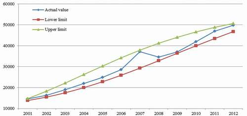
The results in Table 1 show that the proposed RGM(1,1)-NIM is promising because the RGM(1,1)-NIM was superior to the other NIMs considered for both model fitting and ex post testing. Table 2 summarizes the prediction accuracy obtained by applying the NN, autoregressive integrated moving average (ARIMA), GM(1,1), and FLNGM(1,1) to the original data sequence. It is obvious that the RGM(1,1)-NIM was superior to the NN, GM(1,1), and FLNGM(1,1) for ex post testing. The RGM(1,1)-NIM was slightly inferior to GM(1,1) and FLNGM(1,1) for model fitting, but ex post testing is a primary norm used to examine the performance of a prediction model.

The results obtained by ARIMA for ex post testing are encouraging. However, for the first two years (2013 and 2014), the average result obtained by RGM(1,1)-NIM for ex post testing (1.75%) was clearly better than that produced by ARIMA (2.81%). In 2017, the Chinese National Energy Administration released the 13th Five-Year Plan for medium- and long-term energy development to show China’s determination to decrease its environmental impact. Therefore, two years can be roughly treated as a short-term period. Therefore, the proposed RGM(1,1)-NIM can also be used for short-term energy demand forecasting. As mentioned above, the MAREG measures the reasonableness of ${\hat{x}}_{u,k}^{(0)}$ and ${\hat{x}}_{l,k}^{(0)}$ by computing the distance between ${\hat{x}}_{u,k}^{(0)}$ and $x_k^{(0)}$ and that between ${\hat{x}}_{l,k}^{(0)}$ and $x_k^{(0)}$. The results in Table 3 illustrate that data intervals obtained by the proposed RGM(1,1)-NIM are more reasonable than those from the other NIMs considered for ex post testing.

Table 3. MAREG obtained by different NIMs for Case I

Phase	NN-NIM	FLNGM-NIM	IGNPM	GGMM(1,1)	RGM(1,1)-NIM
model-fitting	11.22	13.30	14.21	8.11	10.53
ex post testing	6.46	7.42	16.48	12.36	5.62

Case II

The second experiment was conducted based on the historical annual energy demand of Taiwan using data from the Taiwan Energy Bureau. Data from 2001 to 2012 were used for model fitting, and data from 2013 to 2016 were used for ex post testing. Figure 3 depicts the data intervals determined for model fitting by two NNs.

Figure 3. Lower and upper limits determined by NNs for Case II.

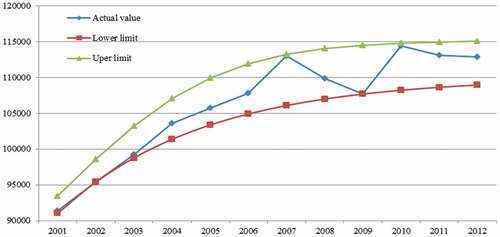
The forecasting results obtained by the various prediction models are summarized in Tables 4 and table 5. These results show that the proposed RGM(1,1)-NIM was slightly inferior to the NN-NIM, NN, and FLNGM(1,1) for model fitting, but it performed better than all the prediction models considered for ex post testing. In terms of the MAREG for ex post testing, Table 6 shows that the reasonableness of the data intervals estimated by the proposed prediction model was slightly inferior to those from the FLNGM-NIM but superior to those from the other NIMs considered.

Table 4. Prediction accuracy obtained by different NIMs for Case II (unit: 10⁴ kLOE)

Year	Actual	NN-NIM		FLNGM(1,1)-NIM		IGNPM		GGMM(1,1)		RGM(1,1)-NIM
		Predicted	APE	Predicted	APE	Predicted	APE	Predicted	APE	Predicted	APE
2001	91333.4	92222.6	0.97	92222.6	0.97	92222.6	0.97	91333.4	0.00	92222.6	0.97
2002	95385.9	96977.9	1.67	97293.0	2.00	96977.9	6.48	97463.4	2.18	97551.31	2.27
2003	99252.5	100972.1	1.73	102674.8	3.45	107376.6	3.63	100689.8	1.45	100772.9	1.53
2004	103553.3	104180.7	0.61	104082.3	0.51	99487.7	0.59	104298.3	0.72	104513.3	0.93
2005	105700.9	106626.1	0.88	105739.0	0.04	109917.2	0.20	106626.8	0.88	107594	1.79
2006	107773.8	108398.4	0.58	107027.0	0.69	102059.5	0.87	109862.2	1.94	109094.2	1.23
2007	113024.6	109638.7	3.00	108561.3	3.95	112520.6	4.27	110826.3	1.95	109370.6	3.23
2008	109819.2	110493.4	0.61	109684.5	0.12	104694.8	0.23	106287.3	3.22	109835.8	0.02
2009	107677	111082.4	3.16	110919.9	3.01	115188.4	3.05	100195.6	6.95	110642	2.75
2010	114368	111492.4	2.51	111582.0	2.44	107395.3	1.74	143562.3	25.53	111898.6	2.16
2011	113105.3	111781.6	1.17	112783.4	0.28	117922.0	0.62	113244.6	0.12	112709.2	0.35
2012	112870.8	111988.6	0.78	113733.0	0.76	110162.6	2.11	114043.2	1.04	113843.8	0.86
MAPE			1.47		1.52		4.07		3.83		1.51
2013	115893.7	112138.8	3.24	115153.0	0.64	120723.2	4.17	114553.4	1.16	115761.3	0.11
2014	116826.5	112249.1	3.92	116136.7	0.59	112998.2	3.28	115079.3	1.50	116881.6	0.05
2015	116509.1	112330.8	3.59	117615.5	0.95	123593.7	6.08	115621.2	0.76	115654.7	0.73
2016	116808.9	112391.9	3.78	118940.7	1.82	115903.9	0.77	116179.3	0.54	115576.8	1.05
MAPE			3.63		1.00		3.57		0.99		0.49

Table 5. Prediction accuracy obtained by different prediction models for Case II (unit: 10⁴ kLOE)

Year	Actual	NN		ARIMA		GM(1,1)		FLNGM(1,1)
		Predicted	APE	Predicted	APE	Predicted	APE	Predicted	APE
2001	91333.4	90894.3	0.48	91333.4	4.24	91333.4	0.00	91333.4	0.00
2002	95385.9	95719.4	0.35	95203.1	4.60	100267.5	5.12	95315.22	0.07
2003	99252.5	99957.2	0.71	99774.9	4.03	101798.4	2.57	100601.9	1.36
2004	103553.3	103408.2	0.14	103256.6	2.27	103352.8	0.19	103278.7	0.27
2005	105700.9	106103.0	0.38	105907.9	2.11	104930.8	0.73	105702.5	0.00
2006	107773.8	108158.0	0.36	107927.1	1.57	106533.0	1.15	107747.7	0.02
2007	113024.6	109704.4	2.94	109464.7	2.11	108159.6	4.30	109379.3	3.23
2008	109819.2	110859.7	0.95	110635.7	1.56	109811.1	0.01	110579.4	0.69
2009	107677	111719.6	3.75	111527.4	4.21	111487.7	3.54	111368.7	3.43
2010	114368	112358.6	1.76	112206.5	1.44	113190.0	1.03	111885.9	2.17
2011	113105.3	112833.4	0.24	112723.6	0.01	114918.3	1.60	112392.1	0.63
2012	112870.8	113186.5	0.28	113117.5	0.48	116672.9	3.37	113147.5	0.25
MAPE			1.03		7.16		1.97		1.01
2013	115893.7	113449.6	2.11	113417.4	1.79	118454.36	2.21	114310.1	1.37
2014	116826.5	113645.9	2.72	113645.8	2.72	120263.00	2.94	115957.9	0.74
2015	116509.1	113792.8	2.33	113819.7	2.31	122099.26	4.80	118145.1	1.40
2016	116808.9	113903.0	2.49	113952.2	2.45	123963.56	6.13	120887.8	3.49
MAPE			2.41		2.40		4.02		1.75

Table 6. MAREG obtained by different NIMs for Case II

Phase	NN-NIM	FLNGM-NIM	IGNPM	GGMM(1,1)	RGM(1,1)-NIM
model-fitting	3.16	3.38	5.26	6.28	3.35
ex post testing	4.39	3.14	5.02	4.36	3.76

Discussion

This study has proposed the RGM(1,1)-NIM, which is made up of two NR-GM(1,1). In particular, the upper and lower RGM(1,1) are created by the NR-GM(1,1). Compared to the other remnant GM(1,1) variants, the NR-GM(1,1) features the ability to leverage the residual model by providing a novel adjustment mechanism for the predicted values to maximize prediction accuracy (Hu 2020). The reason for choosing a value that is three times larger than the max{${\epsilon }_k^{(0)}$} in Eq. (21)(21) $t_l=3max\{{\epsilon }_k^{(0)}\},k=1,2,\dots ,n$(21) is based on the three-sigma limits used to set the upper and lower control limits in statistical quality control charts (Montgomery 2012), thereby making the modification much more flexible.

Real-valued data were collected to verify the prediction accuracy of the proposed RGM(1,1)-NIM. The results showed that the proposed model was superior to the other interval gray prediction models considered for ex post testing. Both the MAPE and MAREG results indicate that the proposed RGM(1,1)-NIM is promising for applications in energy demand forecasting. In addition to RGM(1,1)-NIM, it is interesting to examine forecasting accuracy of the other novel interval models, such as the discrete GM(1,1) of interval gray numbers (Ye et al. 2019) as well by using data intervals generated by two MLPs, but this remains to future study.

This study has focused on forecasting rather than projection. Projection is required to answer “what-if” questions to extrapolate development trends. In other words, it is concerned about what would happen to carbon dioxide emissions based on certain future scenarios. In this case, the key factors that can have the greatest impact on the scenarios must be identified (Norouzi, Fani, and Ziarani 2020b). Besides, Kristjanpoller and Minutolo (2021) point out that the series has underlying characteristics of autocorrelation, heteroskedasticity, and non-linearity. Understanding the cross-correlation relationships between electricity production and demand can boost the performance of the models used to forecast both production and demand. Their findings suggest a way to improve the forecasting performance of the proposed interval model.

Note that the FLN uses the hyperbolic tangent function as its activation function and computes a weighted sum for a connection weight vector with an enhanced pattern. Therefore, such a model assumes the additivity property of the interactions among individual variables in the enhanced pattern (Onisawa et al. 1986). However, the criteria are not always independent (Tzeng and Shen 2017). Therefore, it would be interesting to apply a non-additive version of the FLN (Hu 2017c) to energy demand forecasting in future research.

Conclusions

Energy demand forecasting has played a very important role in economic growth and environmental security. It can be regarded as a gray system problem (Suganthi and Samuel 2012) because factors, such as income and population influence energy demand, but their precise effects are not clear. Therefore, gray prediction, which does not require that data conform to statistical assumptions (Liu and Lin 2010; Liu, Yang, and Forrest 2017), is appropriate for energy demand forecasting. In practice, GM(1,1) forms the development base of the proposed interval model.

The problem addressed in this study is that available energy demand data are usually real-valued, but are uncertain and imprecise. This makes it possible to use nonlinear interval regression analysis with two MLPs, one for the upper limits and the other for the lower limits, to generate interval-valued data to represent uncertainty. Subsequently, the upper and lower RGM(1,1) can be built by working on the data sequences that make up the upper and lower limits, respectively. The experimental results show that the proposed models performed well compared with other interval gray prediction models. The RGM(1,1)-NIM has indicated its high applicability to energy demand forecasting as well.

In Taiwan, almost 98% of energy is imported, and its cost accounts for 13%–15% of the gross domestic product. Furthermore, the energy supply is highly dependent on fossil fuel imports, which are the leading source of high carbon dioxide emissions. The public sectors may leverage the proposed GM to plan an energy development policy to achieve the goals of environmental protection, sustainable economic growth, and green industry development.

Acknowledgments

The authors would like to thank the anonymous referees for their valuable comments. This research is supported by the Ministry of Science and Technology, Taiwan under grant MOST 110-2410-H-033-013-MY2.

Disclosure statement

No potential conflict of interest was reported by the author(s).

Additional information

Funding

This work was supported by the Ministry of Science and Technology, Taiwan [MOST 108-2410-H-033-038-MY2].

References

- Ayoub, N., F. Musharavati, S. Pokharel, and H. A. Gabbar 2018. ANN model for energy demand and supply forecasting in a hybrid energy supply system, 2018 IEEE International Conference on Smart Energy Grid Engineering, Oshawa, Ontario, Canada. doi:https://doi.org/10.1109/SEGE.2018.8499514.
- Braun, M. R., H. Altan, and S. B. M. Beck. 2014. Using regression analysis to predict the future energy consumption of a supermarket in the UK. Applied Energy 130:305–13. doi:https://doi.org/10.1016/j.apenergy.2014.05.062.
- Cankurt, S., and A. Subasi. 2015. Developing tourism demand forecasting models using machine learning techniques with trend, seasonal, and cyclic components. BALKAN Journal of Electrical and Computer Engineering 3 (1):42–49.
- Chen, Y. Y., H. T. Liu, and H. L. Hsieh. 2019. Time series interval forecast using GM(1,1) and NGBM(1, 1) models. Soft Computing 23 (5):1541–55. doi:https://doi.org/10.1007/s00500-017-2876-0.
- Cheng, C. B., and E. S. Lee. 2001. Fuzzy regression with radial basis function network. Fuzzy Sets and Systems 119 (2):291–301. doi:https://doi.org/10.1016/S0165-0114(99)00098-6.
- Cormen, T. H., C. E. Leiserson, R. L. Rivest, and C. Stein. 2009. Introduction to algorithms. Cambridge, MA: MIT Press.
- Dang, Y., S. Liu, and K. Chen. 2004. The GM models that x(n) be taken as initial value. Kybernetes 33 (2):247–54. doi:https://doi.org/10.1108/03684920410514175.
- Forough, A. B., N. Norouzi, and M. Fani. 2021. Investigation of the optimal model for the development of renewable energy in Iran using a Robust Optimization Approach. World Journal of Electrical and Electronic Engineering 1. doi:https://doi.org/10.31586/wjeee.2021.010101.
- Hladík, M., and M. Černý. 2014. Tolerance approach to possibilistic nonlinear regression with interval data. IEEE Transactions on Cybernetics 44 (12):2509–20. doi:https://doi.org/10.1109/TCYB.2014.2309596.
- Hsu, C. C., and C. Y. Chen. 2003. Applications of improved grey prediction model for power demand forecasting. Energy Conversion and Management 44 (14):2241–49. doi:https://doi.org/10.1016/S0196-8904(02)00248-0.
- Hsu, C. I., and Y. U. Wen. 1998. Improved Grey prediction models for trans-Pacific air passenger market. Transportation Planning and Technology 22 (2):87–107. doi:https://doi.org/10.1080/03081069808717622.
- Hsu, L. C. 2003. Applying the grey prediction model to the global integrated circuit industry. Technology Forecasting and Social Change 70 (6):563–74. doi:https://doi.org/10.1016/S0040-1625(02)00195-6.
- Hu, Y. C. 2017a. Grey prediction with residual modification using functional-link net and its application to energy demand forecasting. Kybernetes 46 (2):349–63. doi:https://doi.org/10.1108/K-05-2016-0099.
- Hu, Y. C. 2017b. Electricity consumption forecasting using a neural-network-based grey prediction approach. Journal of the Operational Research Society 68 (10):1259–64. doi:https://doi.org/10.1057/s41274-016-0150-y.
- Hu, Y. C. 2017c. Nonadditive grey prediction using functional-link net for energy demand forecasting. Sustainability 9 (7):1166. doi:https://doi.org/10.3390/su9071166.
- Hu, Y. C. 2020. Energy demand forecasting using a novel remnant GM(1,1) model. Soft Computing 24 (18):13903–12. doi:https://doi.org/10.1007/s00500-020-04765-3.
- Hu, Y. C. 2021. Developing grey prediction with Fourier series using genetic algorithms for tourism demand forecasting. Quality & Quantity 55 (1):315–31. doi:https://doi.org/10.1007/s11135-020-01006-5.
- Huang, L., B. L. Zhang, and Q. Huang. 1998. Robust interval regression analysis using neural networks. Fuzzy Sets and Systems 97 (3):337–47. doi:https://doi.org/10.1016/S0165-0114(96)00325-9.
- Hwang, C., D. H. Hong, and K. H. Seok. 2006. Support vector interval regression machine for crisp input and output data. Fuzzy Sets and Systems 157 (8):1114–25. doi:https://doi.org/10.1016/j.fss.2005.09.008.
- Ishibuchi, H., and H. Tanaka. 1992. Fuzzy regression analysis using neural networks. Fuzzy Sets and Systems 50 (3):257–65. doi:https://doi.org/10.1016/0165-0114(92)90224-R.
- Ishibuchi, H., and M. Nii. 2001. Fuzzy regression using asymmetric fuzzy coefficients and fuzzified neural networks. Fuzzy Sets and Systems 119 (2):273–90. doi:https://doi.org/10.1016/S0165-0114(98)00370-4.
- Jeng, J. T., C. C. Chuang, and S. F. Su. 2003. Support vector interval regression networks for interval regression analysis. Fuzzy Sets and Systems 138 (2):283–300. doi:https://doi.org/10.1016/S0165-0114(02)00570-5.
- Jiang, P., W. B. Wang, Y. C. Hu, H. Jiang, and G. Wu. 2020. Interval grey prediction models with forecast combination for energy demand forecasting. Mathematics 8 (6):960. doi:https://doi.org/10.3390/math8060960.
- Kristjanpoller, W., and M. C. Minutolo. 2021. Asymmetric multi-fractal cross-correlations of the price of electricity in the US with crude oil and the natural gas. Physica A: Statistical Mechanics and Its Applications 572:125830. doi:https://doi.org/10.1016/j.physa.2021.125830.
- Lauret, P., E. Fock, R. N. Randrianarivony, and J. F. Manicom-Ramasamy. 2008. Bayesian neural network approach to short time load forecasting. Energy Conversion and Management 49 (5):1156–66. doi:https://doi.org/10.1016/j.enconman.2007.09.009.
- Lee, S. C., and L. H. Shih. 2011. Forecasting of electricity costs based on an enhanced gray-based learning model: A case study of renewable energy in Taiwan. Technological Forecasting and Social Change 78 (7):1242–53. doi:https://doi.org/10.1016/j.techfore.2011.02.009.
- Lee, Y. S., and L. I. Tong. 2011. Forecasting energy consumption using a grey model improved by incorporating genetic programming. Energy Conversion and Management 52 (1):147–52. doi:https://doi.org/10.1016/j.enconman.2010.06.053.
- Leo, S. D., P. Caramuta, P. Curci, and C. Cosmi. 2020. Regression analysis for energy demand projection: An application to TIMES-Basilicata and TIMES-Italy energy models. Energy 196. doi:https://doi.org/10.1016/j.energy.2020.117058.
- Li, Z., J. Dai, H. Chen, and B. Lin. 2019. An ANN-based fast building energy consumption prediction method for complex architectural form at the early design stage. Building Simulation 12 (4):665–81. doi:https://doi.org/10.1007/s12273-019-0538-0.
- Liu, S., and Y. Lin. 2010. Grey information: Theory and practical applications. London: Springer-Verlag.
- Liu, S., Y. Yang, and J. Forrest. 2017. Grey data analysis: Methods, models and applications. Berlin: Springer.
- Makridakis, S. 1993. Accuracy measures: Theoretical and practical concerns. International Journal of Forecasting 9 (4):527–29. doi:https://doi.org/10.1016/0169-2070(93)90079-3.
- Montgomery, D. C. 2012. Statistical Quality Control: A Modern Introduction. Hoboken, NJ: John Wiley & Sons.
- Nasrabadi, E., and S. M. Hashemi. 2008. Robust fuzzy regression analysis using neural networks. International Journal of Uncertainty, Fuzziness and Knowledge-Based Systems 16 (4):579–98. doi:https://doi.org/10.1142/S021848850800542X.
- Norouzi, N., G. Z. De Rubens, S. Choupanpiesheh, and P. Enevoldsen. 2020c. When pandemics impact economies and climate change: Exploring the impacts of COVID-19 on oil and electricity demand in China. Energy Research & Social Science 68:101654. doi:https://doi.org/10.1016/j.erss.2020.101654.
- Norouzi, N., and M. Fani. 2020. The impacts of the novel Corona virus on the oil and electricity demand in Iran and China. Journal of Energy Management and Technology 4 (4):36–48.
- Norouzi, N., and M. Fani. 2021. Environmental sustainability and coal: The role of financial development and globalization in South Africa. Iranian Journal of Energy and Environment 12 (1):68–80.
- Norouzi, N., M. Fani, and Z. K. Ziarani. 2020a. Black gold falls, black plague arise–An Opec crude oil price forecast using a gray prediction model. Upstream Oil and Gas Technology 5:100015. doi:https://doi.org/10.1016/j.upstre.2020.100015.
- Norouzi, N., M. Fani, and Z. K. Ziarani. 2020b. The fall of oil Age: A scenario planning approach over the last peak oil of human history by 2040. Journal of Petroleum Science and Engineering 188:106827. doi:https://doi.org/10.1016/j.petrol.2019.106827.
- Onisawa, T., M. Sugeno, M. Y. Nishiwaki, H. Kawai, and Y. Harima. 1986. Fuzzy measure analysis of public attitude towards the use of nuclear energy. Fuzzy Sets and Systems 20 (3):259–89. doi:https://doi.org/10.1016/S0165-0114(86)90040-0.
- Shih, C. S., Y. T. Hsu, J. Yeh, and Y. P. Lee. 2011. Grey number prediction using the grey modification model with progression technique. Applied Mathematical Modelling 35 (3):1314–21. doi:https://doi.org/10.1016/j.apm.2010.09.008.
- Suganthi, L., and A. A. Samuel. 2012. Energy models for demand forecasting-A review. Renewable and Sustainable Energy Reviews 16:1223–40.
- Sun, X., W. Sun, J. Wang, Y. Gao, and Y. Gao. 2016. Using a Grey-Markov model optimized by Cuckoo search algorithm to forecast the annual foreign tourist arrivals to China. Tourism Management 52:369–79. doi:https://doi.org/10.1016/j.tourman.2015.07.005.
- Tanaka, H. 1987. Fuzzy data analysis by possibilistic linear models. Fuzzy Sets and Systems 24 (3):363–75. doi:https://doi.org/10.1016/0165-0114(87)90033-9.
- Tanaka, H., S. Uejima, and K. Asai. 1982. Linear regression analysis with fuzzy model. IEEE Transactions on Systems, Man, and Cybernetics 12:903–07.
- Toksari, M. D. 2009. Estimating the net electricity energy generation and demand using ant colony optimization approach: Case of Turkey. Energy Policy 37 (3):1181–87. doi:https://doi.org/10.1016/j.enpol.2008.11.017.
- Tutun, S., C. A. Chou, and E. Canıyılmaz. 2015. A new forecasting framework for volatile behavior in net electricity consumption: A case study in Turkey. Energy 93:2406–22. doi:https://doi.org/10.1016/j.energy.2015.10.064.
- Tzeng, G. H., and K. Y. Shen. 2017. New concepts and trends of hybrid multiple criteria decision making. Boca Raton, FL, USA: CRC Press, NY.
- Wang, C. N., and V. T. Phan. 2015. An improved nonlinear grey Bernoulli model combined with Fourier series. Mathematical Problems in Engineering 2015. Article ID 740272. doi:https://doi.org/10.1155/2015/740272
- Wang, Z. X. 2014. Grey forecasting method for small sample oscillating sequences based on Fourier series. Control and Decision 29 (2):270–74.
- Xia, C., J. Wang, and K. S. McMenemy. 2010. Medium and long term load forecasting model and virtual load forecaster based on radial basis function neural networks. Electrical Power and Energy Systems 32 (7):743–50. doi:https://doi.org/10.1016/j.ijepes.2010.01.009.
- Xie, N., S. Liu, C. Yuan, and Y. Yang. 2014. Grey number sequence forecasting approach for interval analysis: A case of China’s gross domestic product prediction. The Journal of Grey System 26(1): 45–58.
- Xu, N., Y. Dang, and Y. Gong. 2017. Novel grey prediction model with nonlinear optimized time response method for forecasting of electricity consumption in China. Energy 118:473–80. doi:https://doi.org/10.1016/j.energy.2016.10.003.
- Ye, J., Y. Dang, S. Ding, and Y. Yang. 2019. A novel energy consumption forecasting model combining an optimized DGM (1, 1) model with interval grey numbers. Journal of Cleaner Production 229:256–67. doi:https://doi.org/10.1016/j.jclepro.2019.04.336.
- Zeng, B., C. Li, X. Y. Zhou, and X. J. Long. 2014. Prediction model of interval grey number with a real parameter and its application. Abstract and Applied Analysis (2014. doi:https://doi.org/10.1155/2014/939404.
- Zeng, B., S. F. Liu, N. M. Xie, and J. Cui. 2010. Prediction model for interval grey number based on grey band and grey layer. Control and Decision 25 (10):1585–92.