Time Series Analysis of Land Surface Temperature and Drivers of Urban Heat Island Effect Based on Remotely Sensed Data to Develop a Prediction Model

ABSTRACT

The local climate of cities is changing, and one of the primary reasons for this change is rapid urbanization. The Lahore district is situated in the Punjab province of Pakistan and is mainly comprised of Lahore city. This city is among the fastest expanding cities in Pakistan. Due to this rapid urbanization, the natural land surfaces are being altered, harming the local environment and thus causing the urban heat island (UHI) effect. For the analysis of the UHI effect, the fundamental and essential step is assessing the land surface temperature (LST). Therefore, the current investigation assessed LST to evaluate the UHI effect of the Lahore district. This study used the remote sensing data retrieved from the Advanced Spaceborne Thermal Emission and Reflection Radiometer Global Digital Elevation Model (ASTER GDEM) and Moderate-Resolution Imaging Spectroradiometer (MODIS) sensor. Different new generation algorithms were initially used, but a convolutional neural network (CNN) model was used based on the accuracy. The model was developed by utilizing the past 19 years’ LST values along with elevation, road density (RD), and enhanced vegetation index (EVI) as input parameters for analyzing and predicting the LST. The LST data of the year 2020 was used for the validation of the outcomes of the CNN model. Among the model predicted LST and observed LST, a high correlation was noticed. The mean absolute percentage error (MAPE), mean absolute error (MAE), and mean squared error (MSE) for the considered two different periods (January and May) were also computed for both the training and validation processes. The prediction error for most parts of the district was within 0.1 K of the observed values. Hence, the formulated CNN model can be utilized as an essential tool for analyzing and predicting LST and thus for the evaluation of the UHI effect at any location.

Introduction

In present times, a striking shift to urban living is being encountered by humanity. The earth’s environments are facing increasingly strong impacts due to urbanization (Grimm et al. 2008). Moreover, regional climate and weather can be considerably impacted by urbanization (Landsberg 1981). In developing countries, the leading cause of urbanization is high population growth. For instance, Pakistan experienced an increase in the population by 57% from 1996 to 2016 at a yearly increase rate of 2.4% (Imran and Mehmood 2020). Urbanization is regarded as an essential human activity that shows the transition of the natural landscape, which is primarily composed of porous area and vegetation cover, into the impermeable and constructed area (Mathew et al. 2016). This impermeable area is mostly the area that is covered during the construction process by the usage of materials such as bitumen, tiles, bricks, concrete, and roof sheeting. However, the environmental variations triggered by urbanization end up in a surge in the temperature of urban areas than in that of the nearby rural areas, which is an obvious interpretation of environmental deterioration (Landsberg 1981).

During night particularly, the comparative warmness of surfaces of urban areas to nearby natural or non-urbanized land is termed as surface urban heat island (SUHI) effect (Voogt and Oke 2003). For studying the urban atmosphere, an important factor and that among the crucial parameters, which control the biological, chemical, and physical processes of the earth, is the land surface temperature (LST) (Mathew et al. 2019; Pu et al. 2006).

For the surfaces of the earth, the skin temperature can be defined by LST. Furthermore, LST can also be utilized as an express indicator of the UHI effect. The consumption of energy and water increases due to the UHI effect, as indicated by investigations. Primarily during the summer season, the increase in energy demand is mainly attributed to the UHI effect and also the decrease in outside air quality levels. Akbari (1995) demonstrated that for every 1°C surge in the everyday extreme temperature, there is an increase in the peak urban electricity need by almost 2–4% above a threshold of 15–20°C. The usage of air-cooling systems or air conditioners during the summer season is mainly responsible for this increase in energy need. Along with the increase in temperature and electricity utilization, the urban areas also face increased pollutant concentration due to the UHI (Sarrat et al. 2006), and it also influences the regional climatology by forming fog and cloud, increasing humidity, and varying the regional precipitation rate and wind patterns (Taha 1997).

However, at present, the impacts of urbanization on climatology on a continental and global scale can be studied through the introduction of high-resolution earth monitoring satellites. Due to the attributes of satellite imageries such as uniformness, regularity, and extensiveness, they have become an efficient tool in place of ground sensors for UHI studies (Tran et al. 2006). Thermal infrared (TIR) remote sensing is used for recording the temperature through satellites, which involves the computation of the temperature of urban surfaces from the documented radiances by TIR sensors.

The city of Lahore is among the world’s most densely populated cities and is rapidly expanding. In 1996, the urbanization rate of the city was 32.52%, which increased to 36.38% in 2016 (Shirazi and Kazmi 2016). In recent years, the immense change in land use has been caused by this increasing trend. Subsequently, in the urban areas, there is an upsurge in the activities of smog development and air pollution due to the high rate of heat discharge (Levermore et al. 2018). In the Lahore district, the green spots around the urban zones have been decreased by 11% between 2000 and 2009, thus, among the rural and urban areas, resulting in a mean temperature difference of 1–6°C (Shirazi and Kazmi 2016). Even though UHI effects cause amplified heating impacts that boost the worldwide temperature, the UHI effects are localized and are drastically influenced due to the modifications in local climates (Lemus-Canovas et al. 2020). For instance, in Lahore, during the summer (April to August), the increase in daytime air temperature caused severe heatwave incidents from the year 2003 to 2017 (Imran and Mehmood 2020). Thus, considering the current situation of the Lahore district, mitigation of UHI effects is necessary, which necessitates the analysis of past and present patterns of urbanization and land use and their influence on the atmospheric and surface climate and, consequently, development of a prediction model. This investigation has attempted to fill this gap by performing LST assessment and prediction using an advanced deep learning approach for the evaluation of UHI for the Lahore district.

The input variables for LST prediction can be categorized into urban uses and changes along with land geometry (Ahmed et al. 2013; Ranjan et al. 2018). The temporal change in land use/land cover (LULC) is associated with the temporal dynamics of LST. This shows that the surface radiation temperature reaction can be articulated as a function of soil water content and vegetation cover on the surface (Owen et al. 1998). This encouraged several investigations on the correlation between LST and vegetation abundance (Weng 2001; Wu 2004). Many recent studies also found that the land use/land cover (LULC) distribution on the surface of the earth highly influences the LST as contended in previously conducted studies (Bhattacharjee et al. 2013; Buyantuyev and Wu 2010; Fan et al. 2017; Hengl et al. 2012; Hulley et al. 2014; Tsendbazar et al. 2015).

The association between normalized difference vegetation index (NDVI) and LST has been recorded in previous studies (Weng 2001; Weng et al. 2006). An association between the normalized difference built-up index (NDBI) and LST has been documented in the works of Rinner and Hussain (2011) and Chen et al. (2006). Zhao and Chen (2005) and Chen et al. (2006) analyzed the normalized difference bareness index (NDBI) and normalized difference water index (NDWI) for identifying the bareness of soil and delineating the water content in vegetation, respectively. A solid association between LST and NDBI followed by NVDI and NDWI in Suzhou city was founded by Feng et al. (2019).

Additionally, the urban index was observed to have an elevated correlation with LST in Harare, Zimbabwe (Mushore et al. 2017). The pace of building density, land use patterns, and urbanization has a direct relation with the intensity of LST (Ahmed et al. 2013). Some studies contended that the LULC parameter, NDVI, is a weaker forecaster of LST as compared to NDBI, which is a relatively more significant one (Al Rakib et al. 2020; Guha and Govil 2020; Ullah et al. 2019). However, there is still a lot of discussion about the most significant LST parameters because the prospects of various anti-vegetation and vegetation variables to predict LST have established that these variables behave differently as predictors of LST for each area.

Many studies in the past have reported an inverse relationship between LST and vegetation (Gallo and Tarpley 1996; Liu and Notaro 2005; Mathew et al. 2018; Tiangco et al. 2008; Toby 1997; Weng 2001). Cooler temperatures are generated consistently by vegetated areas as compared to non-vegetated pathways, and after plantation, the daily mean temperatures of domestic areas and pathways drop by 0.5 K and 0.9 K, respectively (Yang and Wang 1989). The correlation of LST with vegetation fraction is intensely negative, and this correlation is more intense than the correlation among NDVI and LST (Weng et al. 2004). A negative correlation of LST with vegetation and water in contrast to a compelling positive correlation with roads and buildings was indicated by Liang and Weng (2008). The authors have also observed that with the increase in the geological scale, the correlation among LST and all-terrain parameters enhances and that the larger analytical unit can ensure a sounder correlation among LST and the terrain parameters; thus, better will be the LST modeling. The relationship among LST, NDVI, and percent impervious surface area (%ISA) has been investigated by Yuan and Bauer (2007), and the authors have determined that %ISA is an exact indicator of SUHI effects and demonstrates a solid linear relationship with LST.

Two vegetation indices, NDVI (computed from radiations of near-infrared and visible bands) and enhanced vegetation index (EVI), are included in MODIS products. EVI is computed in the same way as NDVI; however, through a de-coupling of the canopy background signal coupled with a decrease in atmospheric effects, it has improved sensitivity to high biomass regions as well as improved vegetation monitoring (Huete et al. 1999). Atmospherically modified bi-directional surface reflectance (screened for heavy aerosols, water, clouds, and cloud shadows) was used for the computation of the MODIS EVI product. The canopy background variations are minimized by EVI, and it also maintains sensitivity over heavy vegetation situations. The sub-pixel clouds and smoke produced residual atmosphere contamination is also removed by EVI through the utilization of the blue band (USGS).

The LST of an area is affected by the road density (RD) and thus is regarded as one of the important parameters. Among the LSTs and RD, there exists a positive relationship, which implies that where the RD values are highest, the level of urbanization will be maximum. In contrast, EVI values will be the lowest (Mathew et al. 2019). The vegetation cover decreases due to urbanization, and as a result, the surface temperatures escalate (Khandelwal and Goyal 2010). With the change in elevation of various areas, the change in LST has been observed to be changed from the environmental lapse rate. Relying on the moisture situations, the environmental lapse rate fluctuates from 5 to 10°C per 1000 m. For the large areas that have varying ground terrain, the effect of changing LST due to the varying elevation may also be deemed for the UHI investigations. The varying elevation introduces variations in LST, and a contrary relation among elevation and LST for the surrounding area of Jaipur city in India was noted (Khandelwal and Goyal 2010).

Various statistical and/or numerical and machine learning approaches have been used for the prediction of LST in recent times. Sekertekin and Zadbagher (2021) simulated the future form of LST distribution and SUHI evaluation based on the impervious surface area of Zonguldak, a province of Turkey. A multiple linear regression analysis was performed between two indices, normalized difference built-up index (NDBI) and NDVI, and LST to obtain a mathematical prediction model for LST. The future form of the LST image was obtained by simulating these indices using the Markov Chain method, and then, the regression model was employed. Mathew et al. (2019) conducted research for LST prediction for SUHI valuation across Chandigarh city, India, utilizing the Support Vector Regression model. In another investigation, Mathew et al. (2016) predicted the LST for the exploration of the UHI effect over an Indian city of Ahmedabad, exercising the linear time series model. Just like LST, the sea surface temperature (SST) has also been predicted in different studies. Yu et al. (2020) proposed a novel model, integrated Deep Gated Recurrent Unit and Convolutional Neural Network (DGCnetwork), for the prediction of SST. The targeted areas for this research were the East China Sea and the Yellow Sea. Han and Feng et al. (2019) used a convolutional neural network (CNN) for the prediction of subsurface temperatures in the Pacific Ocean using surface data (sea surface salinity, sea surface height, and sea surface temperature). The present research used several new-generation deep learning algorithms (CNN, ResNet, GoogLeNet, and VGGNet). Still, for the representation of the outcomes of prediction of LST, only the better performing model is used. The deep learning technique was used because they have been found superior in terms of feature extraction and prediction accuracy as compared to the orthodox machine learning and statistical techniques.

The primary objective of this investigation was to utilize the association among LST and different influencing parameters, for instance, elevation, RD, and EVI, to formulate a CNN model for the prediction of LST so that the UHI effect on the Lahore district can be evaluated. To perform the LST assessment and develop the CNN model, the study aimed to use multiple remotely sensed data types obtained from multiple sources for two different time periods (January and May). The development of a CNN model in the case of this study can be considered as a method in which the previously mentioned influencing parameters can be linked to establish their impact on LST. As a result, the predicted LST can be utilized to analyze the UHI effect over the Lahore district, as it comprises various influencing parameters that have a direct effect on the LST. The intended analysis is anticipated to be a great deal of help for the planners, as it can be used for effectively planning the development of the city so that the UHI effect can be minimized.

Study area

The district of Lahore was designated as a study area for this research. Comprising a total area of 1,772 km² (684 sq mi), the Lahore district is situated in the Punjab province of Pakistan, primarily comprising of the city of Lahore (area enclosed by the urban boundary), as shown in Figure 1. The city of Lahore, having geographical coordinates 31°32ʹ59ʹʹ N 74°20ʹ37ʹʹ E, is the second biggest metropolitan city of Pakistan and the capital of Punjab province. The population of the district was recorded as over eleven million people during the 2017 census. According to the Pakistan Bureau of Statistics, Lahore ranked 56^th in 1975 and 38^th in 2007 in terms of urban population worldwide, and it is anticipated to be 24^th in 2025. The Lahore district, with a population density of 6,300/km² (16,000/sq mi), is among the most densely populated places in the country. The total area of Lahore that accounts for the green spaces is only 3%, which is far less than the minimum globally required standard for green or open spaces (25–30% of urban area). The two major waterways that run through the district are the Lahore canal and River Ravi. The urban landscape of the district experiences some cooling effects due to these water bodies. Being a central metropolitan, the region has experienced an enormous change in land use in recent years, and even more is expected in the future. Unreliable government strategies, poor land use planning, and swift urbanization according to the residents are the reasons for these changes (Shirazi and Kazmi 2016). The climate of Lahore is semi-arid, with June as the hottest month, when mean highs regularly surpass 40°C (104.0°F). Starting in late June, the monsoon season with intense showers and late afternoon thunderstorms with the chance of rainstorms makes July the wettest month. The month of January is the coolest with heavy fog. The annual average rainfall is 628.8 mm (24.78 inches).

Figure 1. Spatial variation of observed (a) and predicted (b) LST for May.

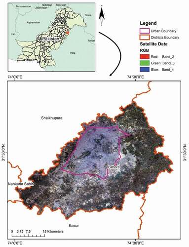
Figure 2. Study area map.

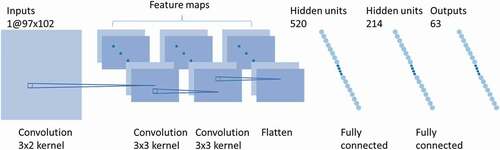
Figure 3. CNN network structure.

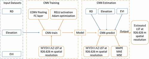
Figure 4. (a) and (b) CNN model methodology.

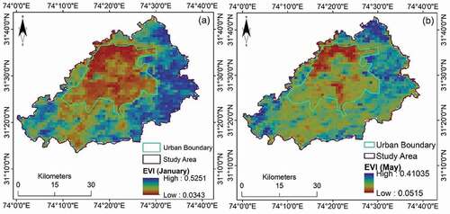
Figure 5. EVI images of the Lahore district of January (a) and May (b) of 2019.

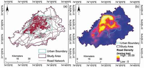
Figure 6. Road network map (a) and road density (b) of the Lahore district.

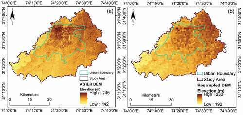
Figure 7. Downloaded ASTER DEM (a) and resampled DEM (b) of the Lahore district.

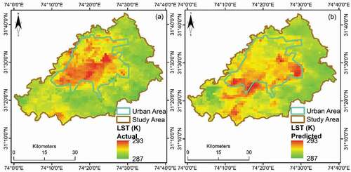
Figure 8. Spatial variation of observed (a) and predicted (b) LST for January.

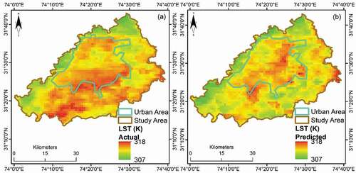
Figure 9. Difference among observed and model-predicted LST for January (009–016).

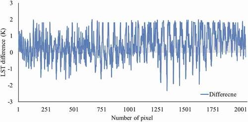
Figure 10. Difference among observed and model-predicted LST for May (137–144).

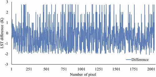
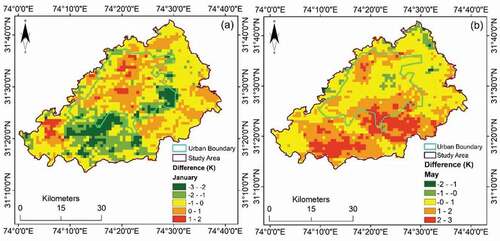
Figure 11. Spatial variation of error between the observed and predicted LST for January (a) and May (b).

Data and methodology

The used remote sensing data products for the current research, the sensor details for each of the products, and the temporal and spatial resolution are presented in Table 1.

Table 1. Used remote sensing data for this study

Remote Sensing Product	Short Name	Sensor	Platform	Temporal Resolution	Spatial Resolution (m)
Land Surface Temperature and Emissivity	MYD11A2	MODIS	Aqua	8-day	926.626
Vegetation Indices	MYD13A2	MODIS	Aqua	16-day	926.626
Land Cover Type	MCD12Q1	MODIS	Combined Aqua and Tera	Yearly	463.3
Digital Elevation Model	ASTGTM	ASTER	Terra	_	24.8

Downloaded LST product

The study used 19-year LST data from 2000 to 2019 to train and test the model. The used images for the research were for two permanent time intervals January (009–016 days) and May (137–144 days) for each of the years from 2000 to 2019. The present study utilized the 8-day, 926.6 m MYD11A2, land surface temperature, and emissivity product of MODIS for two different periods to develop and evaluate the LST prediction results of the model. The available MODIS product comes with a quality flag, and it was examined to incorporate only the excellent quality pixels. In this research, the LST error was limited to 2 K for the analysis.

Input model parameters

Following are the exercised input parameters for the practiced model.

EVI

For the current research, the vegetation indices product of MODIS Aqua (16-day, 926.6 m MYD13A2) of corresponding time periods with the MYD11A2 product was used. Diverse parameters, for instance, the nature of land surface cover that varies from bare ground and vegetation of varying intensity, control the land surface or near-surface temperature. The extent of vegetation throughout an area is indicated by using VI. For SUHI investigations, the MODIS EVI as a depiction of vegetation parameter has been discovered to be a worthier indicator. Therefore, for the formation of the model to predict LST, EVI has been utilized as an input parameter. The EVI images of 19 years for January (001–016 days) and May (129–144 days) have been used in the current research. Single images of these two periods for 19 years have been used. A significant property of EVI is that it possesses the ability to lower atmospheric impacts. Moreover, it also has a soil adjustment factor. It is computed from the reflectance values in near-infrared and red bands, as demonstrated in the equation below

$EVI=2\times \frac{({\rho }_{\mathrm{N}\mathrm{I}\mathrm{R}}-{\rho }_{\mathrm{R}\mathrm{E}\mathrm{D}})}{(L+{\rho }_{\mathrm{N}\mathrm{I}\mathrm{R}}+C_1{\rho }_{\mathrm{R}\mathrm{E}\mathrm{D}}+C_2{\rho }_{BLUE})}$

where ρ is ‘apparent’ (top-of-the-atmosphere) or ‘surface’ directional reflectance, L is a canopy background adjustment term, and C₁ and C₂ weigh the use of the blue channel in the aerosol correction of the red channel (Huete et al. 1994).

RD

Google Earth was used for the preparation of the road network map of the Lahore district. On-screen, digitization of all the roads within the district from Google Earth was performed. All the roads, which are present in the district, either minor or major, have been digitized. The formulated road map was then used for computing the road density of density through the line density tool in the spatial analyst toolbox exercising ArcGIS software. Exploiting the center of the pixel as the circle’s center, the line density was computed as magnitude per unit area of the feature that is contained by a specified radius. Since the size of the LST pixel is 926.626 m, the considered radius for computing RD is 655 m. The circle’s area that has been considered for the computation of RD of a pixel is 57% greater than the area of that pixel.

Elevation

The ASTER GDEM map of the district has been used for obtaining the elevation of the pixels. The produced ASTER DEM standard data products have 30 m postings and Z precisions. Usually, they have a root mean square error (RMSE) between 10 m and 25 m. For producing scene-based DEMs, programmed processing involving stereo-correlation of the ASTER DEM scenes was carried out. The data was made free from the outliers and residual bad values, and then, the final pixel value was created by averaging the preferred data. A correction was made for the residual anomalies, and afterward, the data was segregated into 1 x 1 degree tiles. The natural surface of the earth does not change over a period in terms of elevation, and even it does not experience any huge change as a result of urbanization. The ASTER GDEM of 2011 was used for obtaining the elevation of all the pixels.

MODIS Reprojection Tool (MRT) was used for the pre-processing of the downloaded MODIS images. Moreover, the MRT tools were also utilized for the sub-setting of the MODIS data to a lesser area. Concurrently, from the original sinusoidal projection, the data has also been re-projected to the UTM Zone 43 N projection system with the WGS84 datum, and the format has also been changed from HDF-EOS to GeoTIFF. In GeoTIFF format, afterward, numerous data layers were evaluated utilizing ENVI and ArcGIS software.

Convolutional neural network

As compared to conventional machine learning techniques, the convolutional neural network (CNN) exhibits more intricate network structures as well as more potent feature learning along with feature demonstration capacities (Krizhevsky et al. 2012). Every single neuron is regarded as a filter, slid is the receptive field of each neuron, and the local data is calculated by using a filter. The obtained result of the convolutional layer is operated for a nonlinear mapping operation performed by a rectified linear unit (RELU) excitation layer. Among the consecutive convolutional layers, the pooled layer is sandwiched and is utilized to squeeze the volumes of parameters and data, thus lowering overfitting. Normally, similar to the connection for conventional neural network neurons, the fully connected layer is at the ending of the CNN (Fukushima and Miyake 1982). The parameter update being a slow process is a detriment of CNN. This process necessitates an excessive amount of time to alter the network layer and parameters as per the investigational interpretations. Frequently, the data dimension is reduced by adding the pooling layer, which precedes the damage of significantly useful data. For computation purposes, the CNN always stimulates a small range of data, which disregards the association between the whole and the part. The capability to share weights defines the suitability of CNN, and therefore for a CNN, the network depth is not constrained by the development of parameters.

A mutual convolution core that can efficiently process high-dimensional data and plummet the time of feature engineering by inevitably extricating a few advanced features is regarded as an advantage of CNN (LeCun et al. 1989). This ultimately can enhance the precision of the prediction of surface temperature. Consequently, we intend to utilize CNN to form the model by applying the attributes of 624 data points nearest to the predicted points, which substantially correlated to realistic practicability.

Experimental setup

The whole data was split into the proportion of 70:30 for training and validation purposes, respectively. The data point is treated regarded as a two-dimensional image. For the local field of view, these considered data points perform a convolution operation, whereas the three features (EVI, RD, and elevation) of every data point are operated in one convolution unit. Adam optimization and RELU activation functions were utilized. The established CNN network structure is shown in Figure 2. It is composed of a three-layer convolution operation, followed by a two-layer fully connected layer. For the first layer of the convolution layer, the stride is (3,1); that is, in Figure 2, the horizontal direction moves by three steps, the vertical direction moves by one step. The size of the used filter is 3 × 2. Expressively, the features (EVI, RD, and elevation) of the two data points are multiplied by the related aspects of the filter, and as a result, a sum is achieved. As the calculation of one block area completes, the specific stride (3, 1) is shifted to other areas until a two-dimensional matrix (97 × 102) is entirely contained. As mentioned, data of the entire dataset was divided into a 70–30 ratio for training and validation purposes, and in all datasets for the missing values, the average value for the past year was considered because the localized temperature does not change a lot over the period of short term. Also, to reduce the overfitting problem and set the best possible optimal parameters in the model, a hit and trial method was used by used multiple parameters to see the best possible outcome of the model and parameters gave the best model accuracy, which was used for further analysis. These parameters were optimizers, learning rates, batch size, etc.

The data dimension, following the three-layer convolution operation, was tiled into one-dimensional data, and then, it acted as an input to the fully connected layer. After this, it was subjected to a two-layer neural network operation. Ultimately, the output of this process was the 97 layers of the predicted values. The procedure of assessing the LST by forming a CNN model from remote sensing observation data (EVI, RD, and elevation) is shown in Figure 3. Initially, a training dataset was developed. The feature points that were designated for the training were 1738 data points that were close to the center point and the adjoining data points with the center point. For the test and training markers, the MYD11A2 LST was utilized, plus all the datasets were standardized. Subsequently, the training of the CNN model was performed, and as a result, an ideal CNN model was developed. The RELU is used as an activation function by the model, whereas Adam is used as the optimization function. Every R², MSE, and convergence speed were analyzed so that the ideal combination of the pooled layer, fully connected layer, and convolutional layer can be determined. Used input data for the training of the CNN model were the training data sets (EVI, RD, and elevation), whereas for the training marker, the MYD11A2 LST was utilized. Ultimately, for the prediction of LST, the data sets (EVI, RD, and elevation) were used as the input parameters for the CNN model. Afterward, the LST determined from MODIS data was used to assess the precision of the prediction capability of the CNN model.

Performance assessment

For the evaluation of the performance of the suggested model, the principal statistics employed were mean squared error (MSE) and mean absolute percentage error (MAPE) besides mean absolute error (MAE). The difference among the observed and predicted values for every pixel was taken for the calculation of absolute error (AE) in LST prediction from the model.

$\mathrm{A}\mathrm{E}=|Y-Q|$

where Y and Q denote the observed and predicted LST values, respectively. The MAE was computed by taking the mean of AEs.

$\mathrm{M}\mathrm{A}\mathrm{E}=\frac{AE}{N}$

where

AE = AE₁ + AE₂ + AE₃ + … … … . + AE_n,

AE₁, AE₂, AE₃ … … … .AE_n are absolute errors at each pixel, and

N = the total number of pixels.

MAPE is the mean of absolute percentage errors,

$\mathrm{M}\mathrm{A}\mathrm{P}\mathrm{E}=\frac{\sum ^{PE}}{N}$

where PE represents the percentage error and is computed by dividing AE by the consequent Y value.

Results

Input EVI images for two time periods

The Lahore district’s input EVI images for two periods, January and May from 2000 to 2019, were used as an input parameter along with others to develop the model. However, the EVI images for the two periods, January and May of 2019, are shown in Figure 4(a) and (b), respectively. Those areas that have high vegetation appear blue in the images, whereas those with minute vegetation appear brown and have lower EVI values. For the month of January, with much lower EVI values, the central northern side of the urban area seems significantly darker as compared to the remaining parts, which seem light brown. A very few brown spots can be seen in the rural area, while blue spots, having different intensities representing vegetation growth of variable degree, can be witnessed considerably for the month of May.

Road network and RD of the study area

The road network map of the district is shown in Figure 5(a). The district contains different minor and major roads. The road network in the urban area is more intense than in the rural area, as can be witnessed from the map. The RD image of the Lahore district is shown in Figure 5(b). The image illustrates that the urban area has a higher RD, whereas it is lower in the rural area. The RD of the Lahore district varies from 0 to 35.09 Km/sq. Km.

DEM and resampled DEM of the study area

The elevation of the Lahore district is undulant, with the highest and lowest elevations as 245 m and 142 m, respectively, as can be seen from the DEM of the district presented in Figure 6(a). The resampled ASTER DEM image is shown in Figure 6(b). Following the resampling process, because of the averaging of neighborhood pixels, the lowest elevation increased from 142 m to 192 m, and the highest elevation decreased from 245 m to 232 m.

Accuracy assessment of different algorithms

The accuracy of different used deep learning algorithms for this study is presented in Table 2. It was observed during the training and testing phase that the CNN model outperformed the other used algorithms with an accuracy of 0.87. After CNN, it was VGGNet that achieved an accuracy of 0.84, followed by GooLeNet (0.85) and ResNet (0.81). Hence, based on the achieved accuracy during the modeling process, the present study adopted CNN to present the outcomes of this analysis.

Table 2. Accuracy of different model types

Model Type	Accuracy
ResNet	0.81
GoogLeNet	0.85
VGGNet	0.84
CNN	0.87

Observed and predicted LST for two periods

For January (009–016 days), both the observed and predicted LST images of the Lahore district for the year 2020 are presented in Figure 7(a) and (b), respectively. Similarly, the observed LST image of 2020 and the CNN model predicted LST image for May (137–144 days) are shown in Figure 8 (a) and (b), respectively. The predicted and observed LST images are mean images of January (009–016 days) and May (137–144 days). These figures demonstrate the comparison of spatial variation of the observed and model-predicted LST values. Comparable spatial patterns are exhibited within the urban boundary, as can be observed from both figures. A similar spatial position of the pixels having maximum LST range can be observed inside the urban boundary from the figures. Moreover, a similar pattern can also be observed for the moderate to low LST value pixels near the outer edge of the urban limit.

The high-temperature pixels are indicated by the red color in the figures, and they are mainly in the central part of the district, which comes under the urban area. In comparison, the low-temperature pixels are indicated by the light green color, and they are mainly on the outside boundary of the district, which is the rural area. The area that lies in the urban periphery has a higher LST than the outside area. Moreover, the urban area has the majority of the pixels, which are demonstrating high temperatures. The rural area has a lower LST in contrast to the LST of the urban area.

Descriptive statistics of the observed and predicted LST

The maximum, minimum, mean, and standard deviation for both the observed and predicted LST for both periods are given in Table 3. By comparing the observed and predicted values in the table, it can be noticed that these values are related closely to each other. Moreover, the standard deviation for January is also very close.

Table 3. Comparison of maximum, minimum, and mean actual and predicted LST values for 2020

Month (Day No.)		Status	Maximum	Minimum	Mean	Standard Deviation
January (009–016)	Actual		293.18	286.86	291.15	1.371
	Predicted		293.74	287.25	290.31	1.361
May (137–144)	Actual		317.38	307.14	312.26	1.375
	Predicted		315.98	306.59	311.51	1.428

Comparison of observed and predicted LST values

The plotted graphs showing the difference among the observed and model-predicted LST values for January (009–016 days) and May (137–144 days) for all the pixels (2060) are presented in Figures 9 and Figures 10, respectively. It was noticed that there exists close accordance among the observed and model-predicted LST values for a significant proportion of the measurements. The difference among the observed and model-predicted values for May was observed to be more than the difference for January.

Outcomes of the statistical parameters

For both processes, training and validation of the model, the MAPE, MAE, and MSE are shown in Table 4. As evident from the table, for both periods, the MAE, MAPE, and MSE for training and validation are almost the same. For the two periods January and May, the MAE is 0.29 K and 0.28 K for the training phase and 0.27 K and 0.25 K for the validation phase, respectively. The maximum MAPE is only 0.15%, and MSE is only 0.25, thus demonstrating that the prediction accuracy of the model is high. It means that among the observed and model-predicted values, there is very little variance, and hence a good agreement exists among observed and CNN model predicted values.

Table 4. MAE, MAPE, and MSE for both periods

Data Type	Training		Validation
Month (Day No.)	January (009–016)	May (137–144)	January (009–016)	May (137–144)
MAE (K)	0.29	0.28	0.27	0.25
MAPE (%)	0.14	0.15	0.13	0.14
MSE	0.24	0.25	0.22	0.24

Error in LST prediction

For the study area, the number of pixels categorized as per the error in LST prediction is shown in Table 4. For both periods, the error in prediction for a considerable proportion of pixels of the district is within 0.1 K of the observed LST. Those pixels for which the error is more than 1.0 K of the observed values are relatively less for both periods, and it is only 4% and 13% for January and May, respectively.

For the two time periods, January and May, the spatial disparity of error in the LST prediction is presented in Figure 11(a) and (b), respectively. The pixels with errors in LST prediction are scattered over the whole district, as apparent from the figure. The error among observed and model-predicted LST is more than 0.1 K for very few pixels of the district, as can be witnessed from the figure.

Discussion

The surfaces of the earth experience changes in their structure and materials due to anthropogenic activities. As related to the neighboring natural terrains, the earth’s surface and atmosphere experience alteration in the energy balance and composition due to these changes, respectively. These changes occur through a change process, which is called urbanization. These changes also result in a characterized regional atmosphere of anthropogenic communities called the urban atmosphere (Mathew et al. 2019).

During the starting years of the 20^th century, the population of the world living in cities was only 10% of the then overall population. Presently, it has gone up to around 50% of the existing population, and this fraction of the urban population is expected to soar even further in the upcoming years (Mathew et al. 2016). The surge in the population of urban areas with a related expansion of the economy is triggering enormous enlargement of urban areas, and this also has ensued in the happening of UHI effect over several cities (Cheval and Dumitrescu 2009; Tiangco et al. 2008). Lahore is an important district being the provincial capital located in the Punjab Province, Pakistan. The whole Lahore district is experiencing rapid urbanization, being the hub of regional economic and governmental activities. This change is also substantially influencing the surrounding areas (Imran and Mehmood 2020). Thus, the present study performed an analysis of LST and several associated parameters for the Lahore district to develop an LST prediction model. The study used CNN to perform the analysis based on its accuracy, and a comparison was made among the observed and model-predicted LST. The results indicated that there exists a high correlation between the observed and model-predicted LST.

For the prediction of LST in the current research, a variety of parameters, such as elevation, RD, and EVI, were used. In the EVI images of the district for two periods shown in Figure 4, the EVI values of rural areas relate to a combination of both reaped farming land and vegetated ground. However, the area enclosed by the urban boundary has enormous proportions of built-up and impervious surfaces and a very slight vegetation cover. Moreover, the farming land comprises both the land having bare soil and a slice of the plant left after crop reaping. During the summer spell, particularly during the months of May, June, and July, low water supplies and high temperature result in the decline of vegetation density of the district. That is the reason why the range of EVI values is at a low level.

The road network shown in Figure 5a depicts the effect of urbanization as there is an extensive network of roads in the urban area. On the contrary, as compared to the urban area, the rural area has a very less length of roads in total. The reason for intense RD in the urban area can be the expanded urbanization and the demand for new roads in the area. The DEM and resampled DEM of the Lahore district generated from ASTER DEM data at 24.8 m resolution are presented in Figure 6(a) and (b), respectively. For having a comparison among LST and elevation values, the ASTER DEM image was resampled to the same resolution as that of LST. From Figure 6(a) and (b), Figure 7(a) and (b), and 8(a) and (b) it can be witnessed that for those areas where the LST value is high, the elevation is also high and these areas lie mainly inside the urban boundary. So, from this, it can be said that the elevation has a positive influence on LST. The reason can be that the people tend to dwell in elevated areas to save themselves and their belongings in case of floods and this increases the anthropogenic activities in these areas, which ultimately lead to the increase of temperature. All of these parameters, however, are independent but are associated with each other to some extent. However, each of the parameters, regardless of this association, itself influences the LST distinctively. As the aforementioned parameters are expected to vary individually and maybe to some extent affected by each other, therefore, it is hard to establish interrelatedness.

Consequently, it is imperative to establish the collective influence of these parameters on LST. Hence, for the prediction of LST at any location, the CNN model was built conforming to a set of these parameters: elevation, RD, and EVI. From 2000 to 2019, 19 years of data of elevation, RD, EVI, and LST have been utilized for preparing the 19-year CNN model for the prediction of LST for the year 2020. The ArcGIS software was used for converting the output of the CNN model, which was in the form of discrete data, into image format. The ArcGIS software was also used to derive the LST images from MODIS data.

The fact that how the built-up density of an area influences the LST can be demonstrated by analyzing the rural area (falling outside urban limit) and urban area (falling within the urban limit). The factors that can be attributed to the low temperature in rural areas are low urbanization and greater vegetation. On the contrary, the anthropogenic materials and impervious surfaces present in the urban areas are the reason why they show higher temperature pixels as compared to rural areas. Throughout the two periods for each of the years, the LST pattern does not change considerably over the entire district. For both January and May, from the year 2000 to 2019, an increasing trend of mean LST was observed.

For a particular period, the difference between the maximum and minimum LST of an image is the UHI intensity. The UHI occurs mostly from the alteration of thermodynamic and physical characteristics of urban areas related to the substitution of natural land cover with impervious surfaces and structures. The discharged waste heat from human doings (anthropogenic heat) does exaggerate the UHI. However, it is not the foremost cause (Mathew et al. 2019). The observed and predicted maximum and minimum LST values for two time periods are presented in Table 3.

The predicted values and pixels correlate nicely with the observed values and pixels for both periods: January and May. It is evident from the results of Table 3 along with Figures 7 and 8 that the generated LST values by the CNN model are closely related to the observed values. These outcomes demonstrate that the model possesses a decent ability to describe the alterations in the LST values at distinct pixels of the district, and the model can be utilized for very precise LST prediction. Moreover, the difference between observed LST values and the model predicted LST values were plotted for all the pixels (2060) over the district. The reason for doing this was to have a comparison among the temporal variation of both the observed and model-predicted LST. The model predicts both the lower and higher LSTs with enhanced precision, as can be witnessed from Figures 9 and 10. Furthermore, a comparison has also been made among the observed LST data and model predicted LST for calculating the error, as shown in Table 5 and Figure 11.

Table 5. Number of pixels (% of pixels) of the Lahore district in different error ranges

Month (Day No.)	Between −3 and −2 K	Between −2 and −1 K	Between −1 and 0 K	Between 0 and1 K	Between 1 to 2 K
January (009–016)	186 (9%)	247 (12%)	906 (44%)	639 (31%)	83 (4%)
	Between −2 and −1 K	Between −1 and 0 K	Between 0 and 1 K	Between 1 and 2 K	Between 2 and 3 K
May (137–144)	21 (1%)	123 (6%)	1051 (51%)	597 (29%)	268 (13%)

A positive error represents that the predicted value is less as compared to the observed LST value, while the negative error indicates that the predicted value is higher. The model predicted the LST at various parts of the district very precisely, as evident from Table 5. Those pixels with an error greater than 0.1 k primarily fall out of the urban limit, while in the urban area, the predicted values are very close to the observed values, as can be seen from Figure 11. The reason for this error can be the fact that for the urban area, the EVI values have smaller variations in contrast to the rural area’s EVI values. There is a significant change in the EVI of the rural during various spells along with yearly changes owing to the variations in the concentration of rainfall. The RD may be regarded as one of the reasons for more error in rural areas. One RD data has been exploited for the current research. The rural area might have undergone some development over 19 years, through which certain roads might have been built, therefore causing a variation in the RD. On the other end, the rural area is not expected to have this problem, as the roads there exist before now and normally no additional roads are built or planned after development besides broadening of the roads carried out merely through the subsequent years.

During May, for more pixels of the urban area, the prediction error is beyond 0.1 K as related to January. The reason for this extra error may be the seasonal effect. Since the month of May is during the summer spell as a consequence, it is likely that exceptionally high temperatures are witnessed in the urban area because of the factors such as anthropogenic heat and air pollution (Imran and Mehmood 2020). From the outcomes of the current investigation, it is evident that the LST values generated through the CNN model closely relate to the observed values. The functioning of the CNN model can also be assessed from Table 4, which shows the results of statistical measures computed for both training and validation of the model. Moreover, for the prediction of LST, the proposed model can be utilized as an essential tool when the availability of decent quality LST data through remote sensing interpretations is a problem because of the occurrence of cloud cover or any other disruptions. Thus, it can be deduced that the developed model can be effectively employed for the greatly precise prediction of LST. Consequently, the model can be exploited for the evaluation of the UHI effect.

Conclusion

For the varied nature of the ground surface, the LST has been found to vary and is a critical parameter for various climatological investigations involving investigations on UHI effects. The current investigation aimed at using a formulated CNN model for the analysis and prediction of LST. LST values of 19 years (2000–2019) together with elevation, RD, and EVI as input model parameters were used to train the model. The CNN model was selected among various used models to represent the outcomes of this analysis based on its accuracy. The CNN model outperformed the other models in terms of prediction accuracy. The present study used downloaded LST data from MODIS, and to incorporate only decent quality data for the analysis, the quality flag offered with this data has been employed. From the plotted graphs among observed and predicted LST pixels, it can be concluded that a decent correlation was present among the observed and model-predicted LST values. The values of MAPE, MAE, and MSE of the CNN model for the considered two periods (January and May) were found to be reasonable. Most urban areas exhibited an error of less than 0.1 K, which reveals a close relationship between the observed and model-predicted LST values. The highest error that the application of quality flag has constrained is ±2 K. Since for most parts of the Lahore district, the prediction error of the model was within half of this value and only for May very few pixels of the district have error further than the limited error value, it can be established that the prediction results of the model in terms of LST prediction are very accurate and they can be used for SUHI investigations. Consequently, by utilizing LST images of previous years along with other parameters, LST can be predicted from the CNN model with decent precision. The predicted LST will be valuable in monitoring the SUHI effect. It can be exploited as a valuable tool for organized development of the area, such as curtailing the SUHI effect. Future s^tudies can focus on the prediction of upcoming scenarios of LST using the predicted scenarios of the relevant parameters used with LST.

Acknowledgments

The authors of this research are grateful to the anonymous reviewers for their enlightening comments, which assisted in sharpening the manuscript.

Disclosure statement

No potential conflict of interest was reported by the author(s).

References

- Ahmed, B., Kamruzzaman, M., Zhu, X., Rahman, M., and Choi, K. 2013. Simulating land cover changes and their impacts on land surface temperature in Dhaka, Bangladesh. Remote Sensing. 5(11):5969–98. doi:https://doi.org/10.3390/rs5115969.
- Akbari, H. 1995. “Cooling our communities: An overview of heat island project activities.” Annual Report, Heat Island Group. Lawrence Berkeley National Laboratory. Berkeley.
- Al Rakib, A., Akter, K. S., Rahman, M. N., Arpi, S., and Kafy, A.-A. 2020. Analyzing the pattern of land use land cover change and its impact on land surface temperature: A remote sensing approach in mymensingh, Bangladesh. 1st Int. Student Res. Conf.
- Bhattacharjee, S., Mitra, P., and Ghosh, S. K. 2013. Spatial interpolation to predict missing attributes in GIS using semantic kriging. IEEE Transactions on Geoscience and Remote Sensing. 52(8):4771–80. doi:https://doi.org/10.1109/TGRS.2013.2284489.
- Buyantuyev, A., and J. Wu. 2010. Urban heat islands and landscape heterogeneity: Linking spatiotemporal variations in surface temperatures to land-cover and socioeconomic patterns. Landscape Ecology 25 (1):17–33. doi:https://doi.org/10.1007/s10980-009-9402-4.
- Chen, X.-L., Zhao, H.-M., Li, P.-X., and Yin, Z.-Y. 2006. Remote sensing image-based analysis of the relationship between urban heat island and land use/cover changes. Remote Sensing of Environment. 104(2):133–46. doi:https://doi.org/10.1016/j.rse.2005.11.016.
- Cheval, S., and A. Dumitrescu. 2009. The July urban heat island of Bucharest as derived from MODIS images. Theoretical and Applied Climatology 96 (1):145–53. doi:https://doi.org/10.1007/s00704-008-0019-3.
- Fan, C., Myint, S. W., Kaplan, S., Middel, A., Zheng, B., Rahman, A., . . . Blumberg, D. G. 2017. Understanding the impact of urbanization on surface urban heat islands—A longitudinal analysis of the oasis effect in subtropical desert cities. Remote Sensing. 9(7):672. doi:https://doi.org/10.3390/rs9070672.
- Feng, Y., Gao, C., Tong, X., Chen, S., Lei, Z., and Wang, J. 2019. Spatial patterns of land surface temperature and their influencing factors: A case study in Suzhou, China. Remote Sensing. 11(2):182. doi:https://doi.org/10.3390/rs11020182.
- Fukushima, K., and S. Miyake. 1982. Neocognitron: A self-organizing neural network model for a mechanism of visual pattern recognition. In Competition and cooperation in neural nets, vol. 45, 267–85. Springer, Berlin, Heidelberg.
- Gallo, K., and J. Tarpley. 1996. The comparison of vegetation index and surface temperature composites for urban heat-island analysis. International Journal of Remote Sensing 17 (15):3071–76. doi:https://doi.org/10.1080/01431169608949128.
- Grimm, N. B., Faeth, S. H., Golubiewski, N. E., Redman, C. L., Wu, J., Bai, X., and Briggs, J. M. 2008. Global change and the ecology of cities. science. 319(5864):756–60. doi:https://doi.org/10.1126/science.1150195.
- Guha, S., and H. Govil. 2020. Seasonal impact on the relationship between land surface temperature and normalized difference vegetation index in an urban landscape. In Geocarto International, 1–21. Taylor & Francis.
- Hengl, T., Heuvelink, G. B., Tadić, M. P., and Pebesma, E. J. 2012. Spatio-temporal prediction of daily temperatures using time-series of MODIS LST images. Theoretical and Applied Climatology. 107(1):265–77. doi:https://doi.org/10.1007/s00704-011-0464-2.
- Huete, A., Justice, C., and Liu, H. 1994. Development of vegetation and soil indices for MODIS-EOS. Remote Sensing of Environment. 49(3):224–34. doi:https://doi.org/10.1016/0034-4257(94)90018-3.
- Huete, A., Justice, C., and Van Leeuwen, W. 1999. MODIS vegetation index (MOD 13) algorithm theoretical basis document version 3. In University of arizona, 1200. Vegetation Index and Phenology Lab.
- Hulley, G., Veraverbeke, S., and Hook, S. 2014. Thermal-based techniques for land cover change detection using a new dynamic MODIS multispectral emissivity product (MOD21). Remote Sensing of Environment 140:755–65. doi:https://doi.org/10.1016/j.rse.2013.10.014.
- Imran, M., and A. Mehmood. 2020. Analysis and mapping of present and future drivers of local urban climate using remote sensing: A case of Lahore, Pakistan. Arabian Journal of Geosciences 13 (6):1–14. doi:https://doi.org/10.1007/s12517-020-5214-2.
- Khandelwal, S., and R. Goyal. 2010. Effect of vegetation and urbanization over land surface temperature: Case study of Jaipur City, 177–183. Paris, France: EARSeL Symposium.
- Krizhevsky, A., Sutskever, I., and Hinton, G. E. (2012). Imagenet classification with deep convolutional neural networks. Advances in neural information processing systems.
- Landsberg, H. E. 1981. The urban climate, 84–89. New York, NY, USA: Academic press.
- LeCun, Y., Boser, B., Denker, J. S., Henderson, D., Howard, R. E., Hubbard, W., and Jackel, L. D. 1989. Backpropagation applied to handwritten zip code recognition. Neural Computation. 1(4):541–51. doi:https://doi.org/10.1162/neco.1989.1.4.541.
- Lemus-Canovas, M., Martin-Vide, J., Moreno-Garcia, M. C., and Lopez-Bustins, J. A. 2020. Estimating barcelona’s metropolitan daytime hot and cold poles using landsat-8 land surface temperature. Science of the Total Environment 699:134307. doi:https://doi.org/10.1016/j.scitotenv.2019.134307.
- Levermore, G., Parkinson, J., Lee, K., Laycock, P., and Lindley, S. 2018. The increasing trend of the urban heat island intensity. Urban Climate 24:360–68. doi:https://doi.org/10.1016/j.uclim.2017.02.004.
- Liang, B., and Q. Weng. 2008. Multiscale analysis of census-based land surface temperature variations and determinants in Indianapolis, United States. Journal of Urban Planning and Development 134 (3):129–39. doi:https://doi.org/10.1061/(ASCE)0733-9488(2008)134:3(129).
- Liu, Z., and M. Notaro. 2005. “Assessing global vegetation-climate feedbacks from observations.” AGUFM 2005: B43B-0261.
- Mathew, A., Sreekumar, S., Khandelwal, S., Kaul, N., and Kumar, R. 2016. Prediction of surface temperatures for the assessment of urban heat island effect over Ahmedabad city using linear time series model. Energy and Buildings 128:605–16. doi:https://doi.org/10.1016/j.enbuild.2016.07.004.
- Mathew, A., Khandelwal, S., and Kaul, N. 2018. Analysis of diurnal surface temperature variations for the assessment of surface urban heat island effect over Indian cities. Energy and Buildings 159:271–95. doi:https://doi.org/10.1016/j.enbuild.2017.10.062.
- Mathew, A., Sreekumar, S., Khandelwal, S., and Kumar, R. 2019. Prediction of land surface temperatures for surface urban heat island assessment over Chandigarh city using support vector regression model. Solar Energy 186:404–15. doi:https://doi.org/10.1016/j.solener.2019.04.001.
- Mushore, T. D., Odindi, J., Dube, T., and Mutanga, O. 2017. Prediction of future urban surface temperatures using medium resolution satellite data in Harare metropolitan city, Zimbabwe. Building and Environment 122:397–410. doi:https://doi.org/10.1016/j.buildenv.2017.06.033.
- Owen, T., Carlson, T., and Gillies, R. 1998. An assessment of satellite remotely-sensed land cover parameters in quantitatively describing the climatic effect of urbanization. International Journal of Remote Sensing. 19(9):1663–81. doi:https://doi.org/10.1080/014311698215171.
- Pu, R., Gong, P., Michishita, R., and Sasagawa, T. 2006. Assessment of multi-resolution and multi-sensor data for urban surface temperature retrieval. Remote Sensing of Environment. 104(2):211–25. doi:https://doi.org/10.1016/j.rse.2005.09.022.
- Ranjan, A. K., Anand, A., Kumar, P. B. S., Verma, S. K., and Murmu, L. 2018. Prediction of land surface temperature within Sun City Jodhpur (Rajasthan) in India using integration of artificial neural network and geoinformatics technology. Asian Journal of Geoinformatics 17(3); 14–23.
- Rinner, C., and M. Hussain. 2011. Toronto’s urban heat island—Exploring the relationship between land use and surface temperature. Remote Sensing 3 (6):1251–65. doi:https://doi.org/10.3390/rs3061251.
- Sarrat, C., Lemonsu, A., Masson, V., and Guedalia, D. 2006. Impact of urban heat island on regional atmospheric pollution. Atmospheric Environment. 40(10):1743–58. doi:https://doi.org/10.1016/j.atmosenv.2005.11.037.
- Sekertekin, A., and E. Zadbagher. 2021. Simulation of future land surface temperature distribution and evaluating surface urban heat island based on impervious surface area. Ecological Indicators 122:107230. doi:https://doi.org/10.1016/j.ecolind.2020.107230.
- Shirazi, S. A., and J. H. Kazmi. 2016. Analysis of socio-environmental impacts of the loss of urban trees and vegetation in Lahore, Pakistan: A review of public perception. Ecological Processes 5 (1):5. doi:https://doi.org/10.1186/s13717-016-0050-8.
- Taha, H. 1997. Urban climates and heat islands: Albedo, evapotranspiration, and anthropogenic heat. Energy and Buildings 25 (2):99–103. doi:https://doi.org/10.1016/S0378-7788(96)00999-1.
- Tiangco, M., Lagmay, A., and Argete, J. 2008. ASTER‐based study of the night‐time urban heat island effect in Metro Manila. International Journal of Remote Sensing. 29(10):2799–818. doi:https://doi.org/10.1080/01431160701408360.
- Toby, N. C. 1997. On the relation between NDVI, fractional vegetation cover, and leaf area index. J. Remote Sens. Environ 62 (3):241–52. doi:https://doi.org/10.1016/S0034-4257(97)00104-1.
- Tran, H., Uchihama, D., Ochi, S., and Yasuoka, Y. 2006. Assessment with satellite data of the urban heat island effects in Asian mega cities. International Journal of Applied Earth Observation and Geoinformation. 8(1):34–48. doi:https://doi.org/10.1016/j.jag.2005.05.003.
- Tsendbazar, N.-E., De Bruin, S., Fritz, S., and Herold, M. 2015. Spatial accuracy assessment and integration of global land cover datasets. Remote Sensing. 7(12):15804–21. doi:https://doi.org/10.3390/rs71215804.
- Ullah, S., Tahir, A. A., Akbar, T. A., Hassan, Q. K., Dewan, A., Khan, A. J., and Khan, M. 2019. Remote sensing-based quantification of the relationships between land use land cover changes and surface temperature over the lower himalayan region. Sustainability. 11(19):5492. doi:https://doi.org/10.3390/su11195492.
- Voogt, J. A., and T. R. Oke. 2003. Thermal remote sensing of urban climates. Remote Sensing of Environment 86 (3):370–84. doi:https://doi.org/10.1016/S0034-4257(03)00079-8.
- Weng, Q. 2001. A remote sensing? GIS evaluation of urban expansion and its impact on surface temperature in the Zhujiang Delta, China. International Journal of Remote Sensing 22 (10):1999–2014.
- Weng, Q., Lu, D., and Schubring, J. 2004. Estimation of land surface temperature–vegetation abundance relationship for urban heat island studies. Remote Sensing of Environment. 89(4):467–83. doi:https://doi.org/10.1016/j.rse.2003.11.005.
- Weng, Q., Lu, D., and Liang, B. 2006. Urban surface biophysical descriptors and land surface temperature variations. Photogrammetric Engineering and Remote Sensing. 72(11):1275–86. doi:https://doi.org/10.14358/PERS.72.11.1275.
- Wu, C. 2004. Normalized spectral mixture analysis for monitoring urban composition using ETM+ imagery. Remote Sensing of Environment 93 (4):480–92. doi:https://doi.org/10.1016/j.rse.2004.08.003.
- Yang, S., and S. Wang. 1989. The effect of the afforestation trees in lowering temperatures and enhancing humidity of the air in Guangzhou. Geographical series III. Journal of South China Normal University 1:41–46.
- Yu, X., Shi, S., Xu, L., Liu, Y., Miao, Q., and Sun, M. 2020. A novel method for sea surface temperature prediction based on deep learning. In Mathematical Problems in Engineering, Hindawi, 2020.
- Yuan, F., and M. E. Bauer. 2007. Comparison of impervious surface area and normalized difference vegetation index as indicators of surface urban heat island effects in Landsat imagery. Remote Sensing of Environment 106 (3):375–86. doi:https://doi.org/10.1016/j.rse.2006.09.003.
- Zhao, H., and X. Chen. 2005. Use of normalized difference bareness index in quickly mapping bare areas from TM/ETM±. International geoscience and remote sensing symposium, vol. 3, 1666–1668. Seoul, Korea.