A greenhouse modeling and control using deep neural networks

ABSTRACT

Deep learning approaches have attracted a lot of interest and competition in a variety of fields. The major goal is to design an effective deep learning process in automatic modeling and control field. In this context, our aim is to ameliorate the modeling and control tasks of the greenhouse using deep neural network techniques. In order to emulate the direct dynamics of the system an Elman neural network has been trained and a deep multi-layer perceptron (MLP) neural network has been formed in order to reproduce its inverse dynamics and then used as a neural controller. This later was been associated in cascade with the deep Elman neural model to control the greenhouse internal climate. After performing experiments, simulation results show that the best performances were obtained when we have used a neural controller having two hidden layers and an Elman neural model with two hidden and context layers.

Introduction

ANNs have presented an active research domain over the past decades (Yang and Wang 2020). To produce a standard Neural Network (NN), it is necessary to use neurons providing real-valued activations besides, by adjusting the weights, the NNs is trained. However, the process of learning a NN requires long causal chains of computational steps depending on the problems. Backpropagation using gradient descent algorithm has performed an essential role in NNs since 1980 (Kaviani and Sohn 2020).

ANN, NARX, and RNN-LSTM models were developed in order to predict changes in temperature, humidity, and CO2 that have a direct impact on greenhouse crop growth. As result, RNN-LSTM was the more performant in this task. In addition, various training conditions were analyzed and the prediction performance was determined for time steps from 5 to 30 min. Simulation results prove the potential of applying deep-learning-based prediction models to precision greenhouse control (Jung et al. 2020).

Feed-forward artificial neural networks were developed to link cuticle cracking in pepper and tomato fruit to greenhouse and crop conditions. All data were collected from seven commercial greenhouses in British Columbia, Canada, over a 26-week period. The study proves that artificial neural networks can predict cuticle cracking in greenhouse peppers and tomatoes up to 4 weeks before harvest (Ehret et al. 2008).

A new fault detection method for the wind turbine gearbox was presented. An SVM classifier was implemented to detect the gear fault. To verify the proposed fault detection method, ten-year experimental data from three wind farms in Canada was investigated. Test results prove the accuracy of the proposed fault detection method using the RBF kernel comparing to other kernels and to the MLP network (Kordestani et al. 2020).

An ensemble-based fault isolation scheme was developed to detect and classify faults in a single-shaft industrial gas turbine. To identify the system, a variety of Wiener models based on Laguerre/FIR filters and neural networks were developed. The obtained results show that the presented FDI scheme is correct and accurate (Mousavi et al. 2020).

Adam Glowacz described fault diagnosis method based on analysis of thermal images. Features of thermal images of three electric impact drills (EID) were extracted using the BCAoID. The computed features were analyzed using the Nearest Neighbor classifier and the backpropagation neural network. The recognition results of the performed analysis were in the range of 97.91–100% (Glowacz 2021). He also used the same technique for analysis and classification to evaluate the working condition of angle grinders by means of infrared (IR) thermography and IR image processing. The classification of feature vectors was carried out using two classifiers: Support Vector Machine and Nearest Neighbor. Total recognition efficiency for 3 classes (TRAG) was in the range of 98.5–100% (Glowacz 2021).

Several methods of failure prognosis for condition-based monitoring are described including model-based, data-driven, knowledge-based, and hybrid prognosis methods, which could achieve relatively high accuracy (Mojtaba Kordestani et al. 2019).

Mojtaba Kordestani et al., present a survey of the most common large-scale systems (LSS) architectures. Conventional control schemes, including decentralized, distributed, and hierarchical structures for these LSSs are discussed (Kordestani et al. 2021).

The origin of deep learning came from Artificial Neural Networks (ANNs) study (Hinton, Osindero, and Teh 2006).

Before 2006, it was very difficult to train deep architectures. The main reason, which explains this problem, is the gradient-based optimization with random initialization of weight matrices that has bad results (Bengio et al. 2007). In 2006, GE.Hinton et al. have discovered an effective method for forming deep neural networks, named greedy layer-wise training (Hinton, Osindero, and Teh 2006). This last work opened the first research for machine learning (ML) with deep neural architectures that require deep learning.

Deep learning (DL) is a class of classical machine learning (ML) but with more depth and complexity into the model as well as processing the data using different functions that give a hierarchical representation of the data, through large levels of abstraction (Chen et al. 2020).

Deep learning (DL), support vector machine (SVM), and artificial neural network (ANN) algorithms were used in order to forecast greenhouse gases (GHG) emissions (CO2, CH4, N2O, F-gases, and total GHG) from the electricity production sector in Turkey. According to the results, all algorithms used in the study produce independently satisfying results for forecasting GHG emissions in Turkey (Bakay and Ağbulut 2021).

The most important advantage of Deep Learning is characteristics learning, i.e the Deep learning is able to extract the characteristics from raw data, the characteristics from higher levels being treated by the characteristics of the lower level (LeCun, Bengio, and Hinton 2015).

DL is able to solve more complex problems in particular quickly and well, because of using of more complex models, which allow massive parallelization (Pan and Yang 2010). These complex models used in DL can improve classification accuracy or decrease error in regression problems, if the data sets are large enough to describe the problem.

Deep Learning has become more popular in recent years due to the development of the ability of processing units to compute, although the reducing of the cost: DL algorithms require many computation efforts .The strong computational ability and the low cost allow to perform, train, and implement DL algorithms more fast and easy (Adam P. Piotrowski, Napiorkowski, and Piotrowska 2020).

DL composed of various components (e.g. gates, fully connected layers, activation functions, encode/decode schemes, pooling layers, convolutions, memory cells, etc.), depending on the network architecture used (i.e. Recursive Neural Networks, Unsupervised Pre-trained Networks, Recurrent Neural Networks, Convolutional Neural Networks) (Pan and Yang 2010).

DL architectures such as Deep Boltzmann Machine (DBM), Convolutional Neural Network (CNN), Deep Belief Network (DBN), Recurrent Neural Network (RNN) and Stacked Autoencoder (SAE), have been used successfully in many domains such as medical image analysis (Greenspan, van Ginneken, and Summers 2016; Xu et al. 2014), computer vision (Krizhevsky, Sutskever, and Hinton 2012; Szegedy et al. 2017), driverless car (Chen et al. 2015), and machine health monitoring (Tamilselvan and Wang 2013) and natural language processing (Collobert and Weston 2008; Mikolov et al. 2011).

Deep learning methods have known a great interest and have won several competitions in many domains. Therefore, the most essential task and the principal goal is to create a performant deep learning process in automatic control field. In this context, deep neural network tools are developed in order to improve nonlinear system modeling and control tasks.

The main contributions and novelty of this article are stated as follows.

1. The novelty of this paper is to ameliorate a greenhouse control task using a Deep Elman neural network and a Deep multilayer feed forward neural network.

2. Comparing and discuss the results given in (Fourati and Chtourou 2007) in order to show the accuracy and the efficiency of the proposed technique of the greenhouse modeling and control.

This paper is organized as follows: the considered greenhouse is described in section 2. The greenhouse modeling using a Deep Elman neural network is explained in section 3. The greenhouse control strategy using a Deep feed forward neural controller is presented in section 4. The simulations results of the control step are illustrated in section 5. Finally, the conclusion is presented in section 6.

Greenhouse Presentation

The presented greenhouse is classical, it is composed with glasses armatures, its surface is 40 m² and its volume is 120 m³. The measurements of internal and external climate of the process are done using sensors. The internal hygrometry and internal temperature present the internal climate and the greenhouse outputs. The greenhouse is constituted of actuators that are a sprayer, a curtain defined by a length that varies between 0 and 3 m, a sliding shutter that defined by an opening between 0° and 35° and a heater that works in the on/off mode with 5 kw power.

The considered greenhouse is a complex system with multi-inputs, multi-outputs (MIMO), uncertainty and disturbances. The physical quantities that define its functioning are (Gaudin 1981; Oueslati 1990; Souissi 2002):

• Measurable and controllable input: $Om$ (“curtain”), $Ov$ (“sliding shutter”), $Ch$ (“heating input), $Br$ (“sprayer”).

• Measurable but not controllable input: $He$ (“external hygrometry”),$Te$ (“external temperature”), $Vv$ (“wind speed”), $Rg$ (“global radiant”).

• Outputs: $Ti$ (“internal temperature”), $Hi$ (“internal hygrometry”).

Measurements that define the greenhouse parameters have been taken with 1 minute sampling time through 1 day. This allowed to establish a datafile (database) with 1440 rows, each row is constituted with eight columns that present, the internal temperature $Ti(k)$, the external temperature $Te(k)$, the internal hygrometry $Hi(k)$, the external hygrometry $He(k)$, the sliding shutter $Ov(k)$, the wind speed $Vv(k)$, the shade $Om(k)$, the global radiant $Rg(k)$, the sprayer $Br(k)$ and the heater $Ch(k)$ . The measurements had begun at 0 h (0 min) and finished at 23 h and 59 min (1440 min).

Figure 1 presents a descriptive bloc diagram of the greenhouse.

Figure 1. Descriptive bloc diagram of the greenhouse.

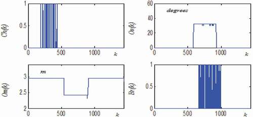
Figure 2 shows the evolution of actuators parameters: Heating ($Ch$), sliding shutter ($Ov$), curtain ($Om$) and sprayer ($Br$).

Figure 2. Evolution of (Heating ($Ch$), sliding shutter ($Ov$), curtain ($Om$) and the sprayer ($Br$).

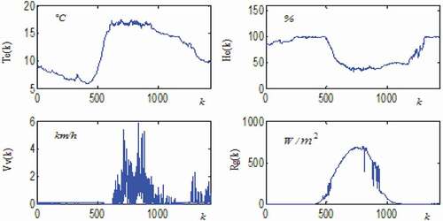
Figure 3 shows the evolution of the external climate: (external temperature ($Te$), external humidity ($He$), Wind speed ($Vv$) and global radiant ($Rg$).

Figure 3. Evolution of (external temperature ($Te$), external hygrometry ($He$), Wind speed ($Vv$) and global radiant ($Rg$).

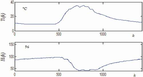
Figure 4 shows the evolution of the greenhouse outputs (the internal climate): Internal temperature ($Ti$) and Internal humidity ($Hi$)).

Figure 4. Evolution of internal temperature ($Ti$) and internal hygrometry ($Hi$)).

Deep Neural Greenhouse Modeling

Greenhouse is a complex system, it requires an efficient tool to be well modeled. For this we have chosen Deep Elman neural network.

Deep Elman Neural Network Architecture

Elman neural network (ENN) was created by Elman in 1990. It is a typical dynamic recurrent network; comparing to traditional neural networks it is particularly composed by an input layer, an output layer, a context layer, a hidden layer (Wang 2020). The principal advantage of ENN resides in the memorization of the previous activations of the nodes hidden by the context nodes, which explains the success of ENN in various fields citing prediction control and dynamic system identification (Chong et al. 2016). The Elman neural network can approximate functions with fast training, large dynamic memory and a limited time (Li et al. 2019). In Elman recurrent neural network (ERNN), the outputs of the hidden layer are used to fed back the information via a recurrent layer (Wang et al. 2019). This feedback makes ERNN to generate, recognize and learn spatial models, as well as temporal models. Each hidden neuron is linked to a single context layer neuron. Consequently, the recurrent layer is in practice a copy of the state of the hidden layer a moment before. As a result, the number of recurrent neurons is equal to the number of hidden neurons. Each layer is constituted by one or more neurons, which send information from one layer to another, by calculating a non-linear function of their weighted sum of inputs (Hongping et al. 2019; Guoa et al. 2019; Yang et al. 2019).

Figure 5 presents a Deep Elman network architecture.

Figure 5. Deep Elman neural network architecture.

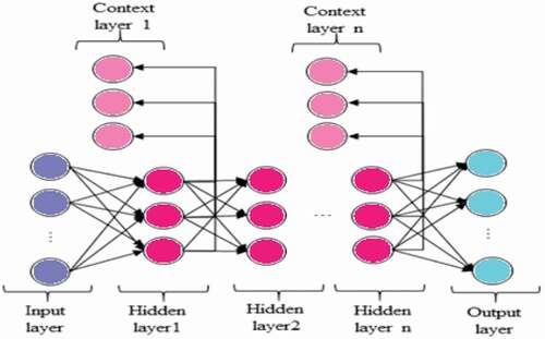
The parameters of the Deep Elman neural network are described as follows:

$V{E}_l(k)$present the total input layer of the network, $y_m(k)$ is the total output layer of the network, $x_i^1(k)$present the total input of first hidden layer of the network, $x_i^{11}(k)$is the total output of first hidden layer of the network, $V_j^c(k)$is the total output of first context layer of the network, $x_{ii}^2(k)$present the total input of second hidden layer of the network, $x_{ii}^{22}(k)$is the total output of second hidden layer of the network, $V_{jj}^{c_2}(k)$ present the total output of second context layer of the network, $x_{i..i}^{n-1}(k)$ is the total input of the (n-1) th hidden layer of the network, $x_{i..i}^{(n-1)(n-1)}(k)$present the total output of the (n-1) th hidden layer of the network, $V_{j..j}^{c_{n-1}}(k)$ is the total output of (n-1) th context layer of the network, $x_{i..ii}^n(k)$ present the total input of the n th hidden layer of the network, $x_{i..ii}^{nn}(k)$is the total output of the n th hidden layer of the network, $V_{j..jj}^{c_n}(k)$ present the total output of the n th context layer of the network, $x_m^s(k)$is the total input of the output layer of the network.

$w_{l,i}^{VE}(.)$present the connection weight which connect the the first hidden layer and the input layer, $w_{i..ii,m}^y(.)$is the connection weight of the output layer and the nth hidden layer, $w_{j,i}^{c_1}(.)$ present the connection weight thats define the links between the first hidden layer and the first context layer, $w_{i,ii}^{x^2}(.)$ present the connection weight of the second hidden layer’ and ‘the first hidden layer, $w_{jj,ii}^{c_2}(.)$ is the connection weight that connects the second hidden layer’ and ‘the second context layer, $w_{i..i,i..ii}^{x^n}(.)$ is the weight connection of the (n-1)th hidden layer’ and ‘the nth hidden layer, $w_{j..jj,i..ii}^{c_n}(.)$ present the connection weight that defines the links between the nth hidden layer’ and ‘the nth context layer.

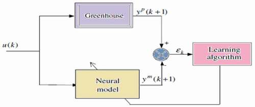
Greenhouse Direct Dynamics Modeling

The training of the deep Elman neural network to reproduce the direct dynamics of the system needs to decrease the squared error criterion presented in (1) as follows:

(1) $E_k=\frac{1}{2}\sum _{m=1}^{n_s}(y{d}_m(k)-y_m(k){)}^2$(1)

$yd(k)$ present the desired output.

The connection weights of the Elman network are adjusted by the using of the back propagation algorithm to model complex systems.

Figure 6 shows the training procedure of a Deep Elman neural network to reproduce the direct dynamics of the considered system (Pham and Liu 1995; Psaltis, Sideris, and Yamamura 1988; Hunt et al. 1992).

Figure 6. Direct dynamics neural modeling.

In the case of many hidden layers, the following equations hold:

(2) ${x^1}_i(k)=\sum _{j=1}^{n_c}{w}_{j,i}^c(k-1)V_j^c(k)+\sum _{l=1}^{n_{VE}}{w}_{l,i}^{VE}(k-1)V{E}_l(k)$(2)

(3) ${x^{11}}_i(k)=f({x^1}_i)$(3)

(4) $V_j^c(k)={x^{11}}_j(k-1)$(4)

(5) ${x^2}_{ii}(k)=\sum _{i=1}^{n_h}{w}_{i,ii}^{x^2}(k-1){x^{11}}_i(k)+\sum _{jj=1}^{n_{c_1}}{w}_{jj,ii}^{c_1}(k-1)V_{jj}^{c_1}(k)$(5)

(6) ${x^{22}}_{ii}(k)=f({x^2}_{ii}(k))$(6)

(7) $V_{jj}^{c_1}(k)={x^{22}}_{jj}(k-1)$(7)

(8) $x_{i..ii}^n(k)=\sum _{i..i=1}^{n_{h_{n-1}}}{w}_{i..i,i..ii}^{x^n}(k-1)x_{i..i}^{(n-1)(n-1)}(k)+\sum _{j..jj=1}^{n_{c_n}}{w}_{j..jj,i..ii}^{c_n}(k-1)V_{j..jj}^{c_n}(k)$(8)

(9) $x_{i..ii}^{nn}(k)=f(x_{i..ii}^n(k))$(9)

(10) $V_{j..jj}^{c_n}(k)=x_{j..jj}^{nn}(k-1)$(10)

(11) $x_m^s(k)=\sum _{i..ii=1}^{n_{h_n}}{w}_{i..ii,m}^y(k-1)x_{i..ii}^{nn}(k)$(11)

(12) $y_m(k)=f(x_m^s)$(12)

where $n_{VE}$ is the number of neurons of the input layer, $n_h$ present the number of unit of the first hidden layer, $n_{c,}$is the number of neurons of the first context layer, $n_{c_1}$ present the number of units of the second context layer, $n_{h_1}$is the number of neurons of the second hidden layer, $n_{h_{n-1}}$present the number of units of the (n-1) th hidden layer, $n_{c_n}$is the number of neurons of the n th context layer and $n_{h_n}$present the number of units of the n th hidden layer.

In the gradient descent method, the general weight adjustment is presented as follows:

(13) $\mathrm{\Delta }w=-\epsilon \frac{\mathrm{\partial }{E}_k}{\mathrm{\partial }w}$(13)

where $\epsilon$ is the learning rate.

The greenhouse datafile is defined in (Fourati and Chtourou 2007). It is divided into two parts, for each parts we have 720 rows. The first part is considered for the learning task and the second part is considered for the validation task.

Here, the input vector is $VE(k)=[Ch(k),Om(k),Ov(k),Br(k),He(k),$$Te(k),Vv(k),Rg(k){]}^T$, and the output vector is $y(k)=[Ti(k),Hi(k)]$ .We consider three neural network structures constituted, respectively, with one single hidden layer, two hidden layers and three hidden layers.

After many tests, we have chosen four units for each hidden and context layers. The learning rate was taken equal to 0.4 ($\epsilon =0.4$). After the training step, the neural network will able to reproduce the greenhouse behavior, then it will be used to accomplish a feed-back control loop.

In order to compare the three neural networks structures we considered the following criterion.

(21) $Et=\sum _{k=1}^{nb}E(k)$(21)

Here, nb = 720.

Figures 7 and 8 present the real internal climate evolution (temperature and hygrometry) where lines are blue and continuous and the outputs of one hidden layer neural network where lines are red and dashed and the considered data file is for the validation task.

Figure 7. Internal temperature evolution.

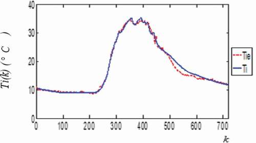
Figure 8. Internal hygrometry evolution.

In this case, $Et=\mathbf{88}.\mathbf{7962}$

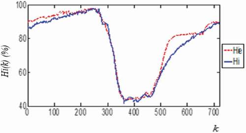
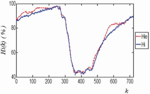
Figures 9 and 10 present the real internal climate evolution (temperature and hygrometry) where lines are blue and continuous and present the outputs of two hidden layers neural network where lines are red and dashed and the considered data file is for the validation task.

Figure 9. Internal temperature evolution.

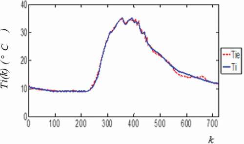
Figure 10. Internal hygrometry evolution.

In this case, $Et=\mathbf{82}.\mathbf{4499}$

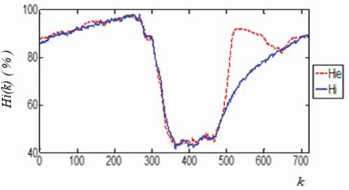
Figures 11 and 12 present the real internal climate evolution (temperature and hygrometry) where lines are blue and continuous and present the outputs of three hidden layers neural network where lines are red and dashed and the considered data file is for the validation task.

Figure 11. Internal temperature evolution.

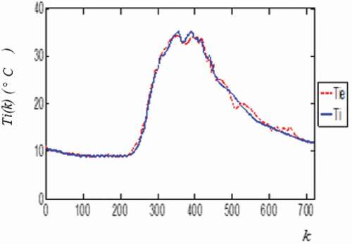
Figure 12. Internal hygrometry evolution.

In this case, $Et=\mathbf{90}.\mathbf{5219}$

The above results show that the neural Elman model with two hidden and context layers has emulated ″perfectly″ the direct dynamics of the system. It can be used to the control task efficiently.

Deep Neural Greenhouse Control Strategy

In this section, the real greenhouse is changed by the Deep Elman neural network model defined previously. The controller that we need must has the capacity to take with the non-linearity of the process in order to control the greenhouse. For this reason, The Deep multilayer feed-forward neural network constituted with an input layer, an output layer and n hidden layers present a solution to control such system (Pham and Liu 1995; Psaltis, Sideris, and Yamamura 1988; Hunt et al. 1992).

Deep Neural Controller Structure

Psaltis et al.’s multilayered neural network controller has known a great success on neural control. It is a feed forward neural network. It gives a large architecture for control and it is defined by its capacity to learn complexes input-output relationships from data (Wang et al. 2018).

The Deep feed forward neural network composed with an input layer, an output layer, and n hidden layer has the capacity to take with the non-linearity to control the greenhouse.

Figure 13 presents the architecture of a Deep feed forward neural network.

Figure 13. Architecture of a Deep feed-forward neural network.

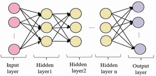
The parameters of the Deep feed forward neural network are described as follows:

$I{n}_l(k)$ present the total input of the network, $O{u}_m(k)$is the total output of the network, $I{n}_i^1(k)$present the total input of first hidden layer of the network, $I{n}_i^{11}(k)$ is the total output of first hidden layer of the network, $I{n}_{ii}^2(k)$present the total input of second hidden layer of the network, $I{n}_{i..i}^{n-1}(k)$ is the total input of (n-1th) hidden layer of the network, $I{n}_{i..i}^{(n-1)(n-1)}(k)$ present the total output of (n-1th) hidden layer of the network, $I{n}_{i..ii}^n(k)$is the total input of (n th) hidden layer of the network, $I{n}_{i..ii}^{nn}(k)$ present the total output of (n th) hidden layer of the network, $I{n}_m^s(k)$ is the total input of output layer of the network.

$w_{l,i}^{In}(.)$present the connection weight which define the links between the the input layer’ and ‘the first hidden layer, $w_{i..ii,m}^{Ou}(.)$ is the connection weight of the the output layer’ and ‘the (n th) hidden layer, $w_{i,ii}^{I{n}^2}(.)$ is the connection weight that connects the second hidden layer’ and ‘the first hidden layer, $w_{i..i,i..ii}^{I{n}^n}(.)$ present the connection weight of the (n-1)th hidden layer’ and ‘the nth hidden layer.

Deep Neural Controller Training

In this step, the training structure used is like to an offline learning to emulate the inverse dynamics of the greenhouse. The used neural network is a Deep feed forward neural network kind (Wang et al. 2018; Cabera and Narendra 1999; Levin and Narendra 1993). Figure 14 presents the training method of the neural controller.

Figure 14. Deep feed-forward neural controller training.

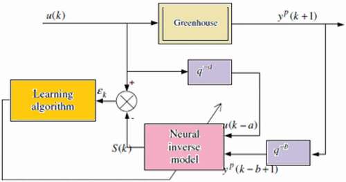
Here, In(k) present the input vector of the controller is:

$In(k)=$ $In(k)=[Ti(k+1),Hi(k+1),Ti(k),Hi(k),Te(k),He(k),Vv(k),Rg(k){]}^T$

Ou(k) is the output vector (control law):

$Ou(k)=U(k)=[Br(k),Ch(k),Ov(k),Om(k){]}^T$

The neural network is trained for minimizing the quadratic error criterion E (k) (22) between the greenhouse input U(k) and the output estimated by the neural network Û (k).

(22) $E(k)=\frac{1}{2}(U(k)-\hat{U}(k){)}^2$(22)

The neural network is presented by the following equations:

(23) $I{n}_i^1(k)=\sum _{l=1}^{n_{In}}{w}_{l,i}^{In}(k-1)I{n}_l(k)$(23)

(24) $I{n}_i^{11}(k)=f(I{n}_i^1(k))$(24)

(25) $I{n}_{ii}^2(k)=\sum _{i=1}^{n_h}{w}_{i,ii}^{I{n}^2}(k-1)I{n}_i^{11}(k)$(25)

(26) $I{n}_{ii}^{22}(k)=f(I{n}_{ii}^2(k))$(26)

(27) $I{n}_{i..ii}^n(k)=\sum _{i..i=1}^{n_{h_{n-1}}}{w}_{i..i,i..ii}^{I{n}^n}(k-1)I{n}_{i..i}^{(n-1)(n-1)}(k)$(27)

(28) $I{n}_{i..ii}^{nn}(k)=f(I{n}_{i..ii}^n(k))$(28)

(29) $I{n}_m^s(k)=\sum _{i..ii=1}^{n_{h_n}}{w}_{i..ii,m}^{Ou}(k-1)I{n}_{i..ii}^{nn}(k)$(29)

(30) $O{u}_m(k)=f(I{n}_m^s(k))$(30)

where $n_{In}$ is the number of neurons of the input layer, $n_h$ present the number of unit of the first hidden layer, $n_{h_1}$is the number of units of the second hidden layer, $n_{h_{n-1}}$present the number of neurons of the (n – 1) th hidden layer and $n_{h_n}$is the number of units of the nth hidden layers.

f is a sigmoidal function:

(31) $f(x)=\frac{1}{1+e^{-x}}$(31)

The learning step requires to adjust the connection weights using the back propagation algorithm by decreasing the criterion (21) by the gradient method.

(32) $w(t)=w(t-1)+\mathrm{\Delta }w$(32)

and

(33) $\mathrm{\Delta }w=-\eta \frac{\mathrm{\partial }{E}_k}{\mathrm{\partial }w}$(33)

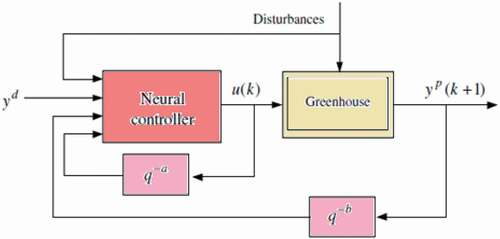
Control Structure

After training, the deep neural controller has the ability to give an accurate $U(k)$ to the greenhouse when the desired output is specified. In Figure 16 The Deep neural controller is located in cascade with the considered greenhouse, where the whole system is a feedback control. The desired output is$Sd(k)=[Tid(k),Hid(k){]}^T=[11,70{]}^T$. An hygrometry $Hid(k)=70\mathrm{\%}$ and a temperature $Tid(k)={11}^{o}C$ are the references represented from agriculturists.

The control strategy has been done to the greenhouse described by the Elman neural network model. Figures 15 and 16 show, respectively, the controller bloc diagram and the used neural control strategy.

Figure 15. Controller bloc diagram.

Figure 16. Neural control strategy.

Simulations Results

We consider three neural network structures constituted, respectively, with one single hidden layer, two hidden layers and three hidden layers.

We use the criterion (21) in order to compare results given from the three neural network structures.

The evolution of the greenhouse outputs and actuators actions using a neural controller and an Elman neural network model with one hidden layer are given in Figures 17-20.

Figure 17. Internal humidity evolution.

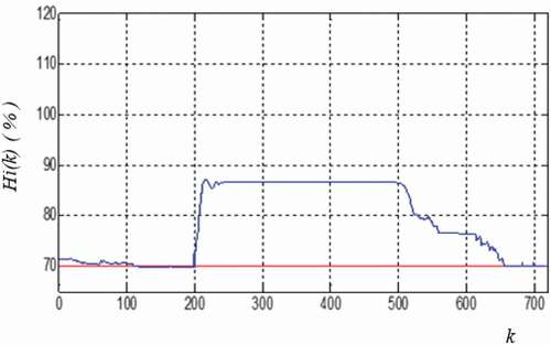
Figure 18. Internal temperature evolution.

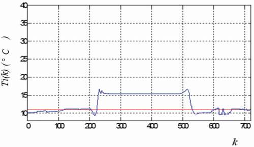
Figure 19. Evolution of the heater and the sliding shutter actuators.

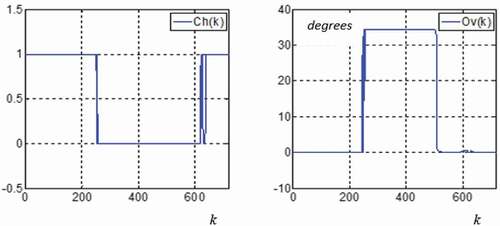
Figure 20. Evolution of the sprayer and curtain actuators.

In this case, $Et=\mathbf{136}.\mathbf{75}$

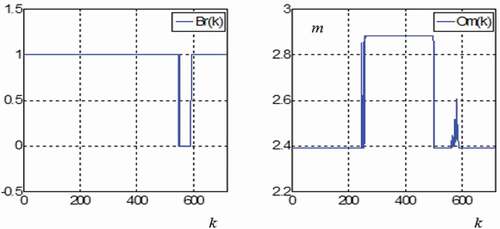
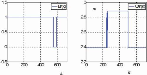
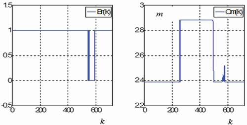
The evolution of the greenhouse outputs and actuators actions using a neural controller and an Elman neural network model constituted with two hidden layers are given in Figures 21-24.

Figure 21. Internal humidity evolution.

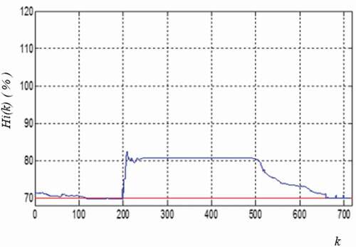
Figure 22. Internal temperature evolution.

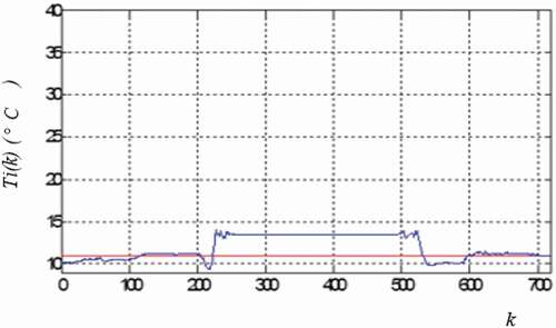
Figure 23. Evolution of the heater and the sliding shutter actuators.

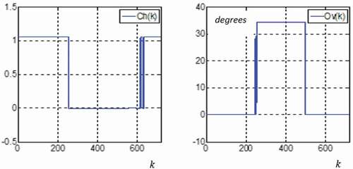
Figure 24. Evolution of the sprayer and curtain actuators.

In this case, $Et=\mathbf{129}.\mathbf{89}$

The evolution of the greenhouse outputs and actuators actions using a neural controller and an Elman neural network model constituted with three hidden layers are given in Figures 25-28.

Figure 25. Internal humidity evolution.

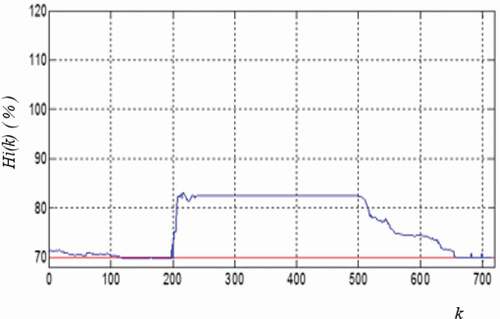
Figure 26. Internal temperature evolution.

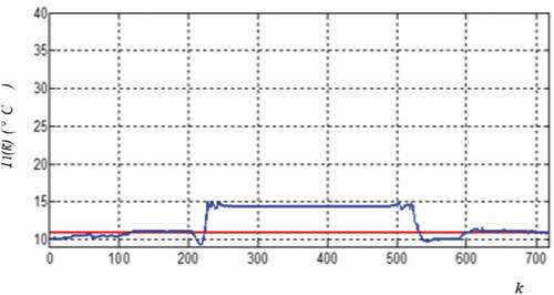
Figure 27. Evolution of the heater and the sliding shutter actuators.

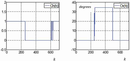
Figure 28. Evolution of the sprayer and curtain actuators.

In this case, $Et=\mathbf{133}.\mathbf{45}$

From the previous results, we conclude that the error criterion is lower when we use a neural controller and an Elman neural network constituted with two hidden layer, adding to that the greenhouse outputs seem more suitable and stable.

In comparison to (Fourati and Chtourou 2007), they used an Elman-type RNN to simulate greenhouse dynamics. In addition, for greenhouse control, they created an FFNN with an inverse learning process. In the greenhouse control, they connected both NNs in a cascade, resulting in a lower criterion error (Et = 344.12), whereas in our case Et = 129.89 for the network with two hidden layers. As a result, the error criterion decreases by using deep neural networks methods. Therefore, the proposed technique adapt well and it is used to enhance greenhouse control.

Conclusion

In this paper, we used a Deep Elman neural network to model the greenhouse. This neural model is then used to simulate the direct dynamics of the greenhouse under consideration. Then, to simulate the greenhouse inverse dynamics, a Deep multilayer feed forward neural network was trained. Both deep neural networks were linked together in a cascade to achieve deep neural control of the greenhouse. The simulation results show that the adopted control strategy was improved by using an Elman neural network and a feed forward neural controller composed each of them of two hidden layers. In fact, the evaluation error criterion Et was weaker in this case than in all others. Therefore, the main advantage of the proposed method resides in the accuracy and efficiency of the obtained results of modeling and control of the greenhouse.

More than one perspective is given, influenced by the results of this study. These perspectives can be summarized as follows:

• Multiple deep neural control

• Control with specialized learning

• Control with generalized learning

Disclosure Statement

No potential conflict of interest was reported by the author(s).

References

- Bakay, M. S., and Ü. Ağbulut. 2021. Electricity production based forecasting of greenhouse gas emissions in Turkey with deep learning, support vector machine and artificial neural network algorithms. Journal of Cleaner Production 285:125324. doi:https://doi.org/10.1016/j.jclepro.2020.125324.
- Bengio, Y., P. Lamblin, D. Popovici, and H. Larochelle. 2007. Greedy layer-wise training of deep networks. Advances in Neural Information Processing Systems 153–60.
- Cabera, J. B. D., and K. S. Narendra. 1999. Issues in the application of neural networks for tracking based on inverse control. IEEE Transactions on Automatic Control 44 (11):2007–27. doi:https://doi.org/10.1109/9.802910.
- Chen, C., A. Seff, A. Kornhauser, J. Xiao, and Deepdriving .2015. Learning affordance for direct perception in autonomous driving. Proceedings of the IEEE International Conference on Computer Vision, 2722–30.
- Chen, Y., Y. Xie, L. Song, F. Chen, and T. Tang. 2020. A survey of accelerator architectures for deep neural networks. Engineering 6 (3):264–74. doi:https://doi.org/10.1016/j.eng.2020.01.007.
- Chong, S., S. Rui, L. Jie, Z. Xiaoming, T. Jun, S. Yunbo, L. Jun, and C. Huiliang. 2016. Temperature drift modeling of MEMS gyroscope based on genetic-Elman neural network. Mechanical Systems and Signal Processing 72:897–905. doi:https://doi.org/10.1016/j.ymssp.2015.11.004.
- Collobert, R., and J. Weston. 2008. A unified architecture for natural language processing: Deep neural networks with multitask learning. Proceedings of the 25th international conference on Machine learning, ACM, 160–67.
- Ehret, D. , B. Hill, D. Raworth, and B. Estergaard. 2008. Artificial neural network modelling to predict cuticle cracking in greenhouse peppers and tomatoes. Computers and Electronics in Agriculture 61 (2):108–16. doi:https://doi.org/10.1016/j.compag.2007.09.011.
- Fourati, F., and M. Chtourou. 2007. A greenhouse control with feed-forward and recurrent neural networks. Simulation Modelling Practice and Theory 15 (8):1016–28. doi:https://doi.org/10.1016/j.simpat.2007.06.001.
- Gaudin, V. C. 1981. “Simulation et commande auto-adaptative d’une serre agricole. Ph.D. Thesis, University of Nantes.
- Glowacz, A. 2021a. Ventilation diagnosis of angle grinder using thermal imaging. Sensors 21 (8):2853. doi:https://doi.org/10.3390/s21082853.
- Glowacz, A. 2021b. Fault diagnosis of electric impact drills using thermal imaging. Measurement 171:108815. doi:https://doi.org/10.1016/j.measurement.2020.108815.
- Greenspan, H., B. van Ginneken, and R. M. Summers. 2016. Guest editorial deep learning in medical imaging: Overview and future promise of an exciting new technique. IEEE Transactions on Medical Imaging 5:1153–59. doi:https://doi.org/10.1109/TMI.2016.2553401.
- Guoa, C., J. Luc, Z. Tiana, W. Guob, and A. Darvishand. 2019. Optimization of critical parameters of PEM fuel cell using TLBO-DE based on Elman neural network. Energy Conversion and Management 183:149–58. doi:https://doi.org/10.1016/j.enconman.2018.12.088.
- Hinton, G. E., S. Osindero, and Y.-W. Teh. 2006. A fast learning algorithm for deep belief nets. Neural Computation 7:1527–54. doi:https://doi.org/10.1162/neco.2006.18.7.1527.
- Hongping, H., H. Wang, Y. Bai, and M. Liu. 2019. Determination of endometrial carcinoma with gene expression based on optimized Elman neural network. Applied Mathematics and Computation 341:204–14. doi:https://doi.org/10.1016/j.amc.2018.09.005.
- Hunt, K. J., D. Sbarbaro, R. Zbikowski, and P. J. Gawthrop. 1992. Neural networks for control systems—a survey. Automatica 28 (6):1083–112. doi:https://doi.org/10.1016/0005-1098(92)90053-I.
- Jung, D.-H., H. S. Kim, C. Jhin, H.-J. Kim, and S. H. Park. 2020. Time-serial analysis of deep neural network models for prediction of climatic conditions inside a greenhouse. Computers and Electronics in Agriculture 173:10540. doi:https://doi.org/10.1016/j.compag.2020.105402.
- Kaviani, S., and I. Sohn. 2020. Influence of random topology in artificial neural networks: A survey. ICT Express 6 (2):145–50. doi:https://doi.org/10.1016/j.icte.2020.01.002.
- Kordestani, M., M. Rezamand, M. Orchard, R. Carriveau, D. S. K. Ting, and M. Saif. 2020. Planetary gear faults detection in wind turbine gearbox based on a ten years historical data from three wind farms. IFAC-PapersOnLine 53 (2):10318–23. doi:https://doi.org/10.1016/j.ifacol.2020.12.2767.
- Kordestani, M., A. A. Safavi, and M. Saif. 2020. Recent survey of large-scale systems: architectures, controller strategies, and industrial applications. IEEE Systems Journal 3048951.
- Kordestani, M., M. Saif, M. Orchard, R. Razavi-Far, and K. Khorasani. 2021. Failure prognosis and applications—a survey of recent literature. IEEE Transactions on Reliability 70 (2):728–48. doi:https://doi.org/10.1109/TR.2019.2930195.
- Krizhevsky, A., I. Sutskever, and G. E. Hinton. 2012. Imagenet classification with deep convolutional neural networks. Advances in Neural Information Processing Systems 1:1097–105.
- LeCun, Y., Y. Bengio, and G. Hinton. 2015. Deep learning. Nature 521 (7553):436–44. doi:https://doi.org/10.1038/nature14539.
- Levin, A. U., and K. S. Narendra. 1993. Control of nonlinear dynamical systems using neural networks: Controllability and stabilization. IEEE Transactions on Neural Networks 4 (2):192–206. doi:https://doi.org/10.1109/72.207608.
- Li, W., Z. Jiao, L. Du, W. Fan, and Y. Zhu. 2019. An indirect RUL prognosis for lithium-ion battery under vibration stress using Elman neural network. International Journal of Hydrogen Energy 44 (23):12270–76. doi:https://doi.org/10.1016/j.ijhydene.2019.03.101.
- Mikolov, T., M. Karafi´at, L. Burget, J. Cernock`y, and S. Khudanpur. 2011. Recurrent neural network based language model. Interspeech 2877–80.
- Mousavi, M., M. Moradi, A. Chaibakhsh, M. Kordestani, and M. Saif. 2020. Ensemble-based fault detection and isolation of an industrial gas turbine. 2020 IEEE International Conference on Systems, Man, and Cybernetics (SMC), 2351–58.
- Oueslati, L. 1990. Commande multivariable d’une serre agricole par minimisation d’un crite`re quadratique. Ph.D. Thesis, University of Toulon, Toulon.
- Pan, S. J., and Q. Yang. 2010. A survey on transfer learning. IEEE Transactions on Knowledge and Data Engineering 22 (10):1345–59. doi:https://doi.org/10.1109/TKDE.2009.191.
- Pham, D. T., and X. Liu. 1995. Neural networks for identification. In Prediction and control. London: Springer.
- Piotrowski, A., J. Napiorkowski, and A. Piotrowska. 2020. Impact of deep learning-based dropout on shallow neural networks applied to stream temperature modelling. Earth-Science Reviews 201:103076. doi:https://doi.org/10.1016/j.earscirev.2019.103076.
- Psaltis, D., A. Sideris, and A. A. Yamamura. 1988. A multilayer neural network controller. IEEE Control Systems Magazine 8 (2):17–21. doi:https://doi.org/10.1109/37.1868.
- Souissi, M.2002. Mode´lisation et commande du climat d’une serre agricole. Ph.D. Thesis, University of Tunis, Tunis.
- Szegedy, C., S. Ioffe, V. Vanhoucke, and A. A. Alemi. 2017. Inception-v4, inception-resnet and the impact of residual connections on learning. AAAI 4278–84.
- Tamilselvan, P., and P. Wang. 2013. Failure diagnosis using deep belief learning based health state classification. Reliability Engineering & System Safety 115:124–35. doi:https://doi.org/10.1016/j.ress.2013.02.022.
- Wang, C., W. Zhao, Z. Luan, Q. Gao, and K. Deng. 2018. Decoupling control of vehicle chassis system based on neural network inverse system. Mechanical Systems and Signal Processing 106:176–97. doi:https://doi.org/10.1016/j.ymssp.2017.12.032.
- Wang, J., Z. Lv, Y. Liang, L. Deng, and Z. Lia. 2019. Fouling resistance prediction based on GA–Elman neural network for circulating cooling water with electromagnetic anti-fouling treatment. Journal of the Energy Institute 92 (5):1519–26. doi:https://doi.org/10.1016/j.joei.2018.07.022.
- Wang, J. 2020. A deep learning approach for atrial fibrillation signals classification based on convolutional and modified Elman neural network. Future Generation Computer Systems 102:670–79. doi:https://doi.org/10.1016/j.future.2019.09.012.
- Xu, Y., T. Mo, Q. Feng, P. Zhong, M. Lai, I. Eric, and C. Chang. 2014. Deep learning of feature representation with multiple instance learning for medical image analysis. IEEE International Conference on Acoustics, Speech and Signal Processing (ICASSP), 1626–30.
- Yang, G. R., and X.-J. Wang. 2020. Artificial neural networks for neuroscientists: a primer. Neuron 107 (6):1048–70. doi:https://doi.org/10.1016/j.neuron.2020.09.005.
- Yang, L., F. Wang, J. Zhang, and W. Ren. 2019. Remaining useful life prediction of ultrasonic motor based on Elman neural network with improved particle swarm optimization. Measurement 143:27–38. doi:https://doi.org/10.1016/j.measurement.2019.05.013.