A Convolutional Neural Network for Detecting Faults in Power Distribution Networks along a Railway: A Case Study Using YOLO

ABSTRACT

This work presents a Convolutional Neural Network (CNN) called YOLO for detecting failures in components of power lines along a railway. The task is a significant challenge because the CNN has to recognize the object and then classify it in real-time. Moreover, some extra difficulties are presented in the task, such as similarity in terms of color, the intersection of components, the component size, and climate conditions. The failure scenarios have been simulated in a laboratory containing all the structures found in real-world power lines along railways. The laboratory allowed us to build the image dataset containing $708$ images with annotations that have been used for training the neural network. Three versions of the Yolo V3 were compared against the state-of-the-art convolutional neural network called Tiny Yolo. Results have shown that Yolo V3 version 2 adequately detects the objects and faults, reaching a precision of $98\mathrm{\%}$, a recall of $95\mathrm{\%}$, and a MAP of $96.58\mathrm{\%}$.

Introduction

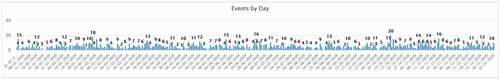
An electric system is a complex structure that provides consumers with power, such as houses, industries, and railways, in the context of this work. Inside an electrical distribution network, we can find different components, such as arresters, transforms, cross arms, etc. These components are located in the power posts and are subject to faults caused by regular operation, climatic conditions, or vandalism. In this context, Figure1 shows the distribution of the railway events (failures) related to power components in 2020 that totalized $1975$ episodes. As we can see, the number of occurrences is high and cannot be neglected because it can represent a high cost to the company that maintains the power line.

Figure1. Electrical distribution components – related events in 2020.

To minimize the effect of faults on consumers, it is essential to have a contingency plan or avoid failure before it happens. The second option is definitively the best because the consumer does not suffer from a lack of power and, consequently, with the service’s unexpected interruption. In extreme cases, the supplier can notify the consumers about a scheduled power supply interruption, reducing their effect. Anyhow, the failure to supply power can cause financial loss to the consumer even if there is a previous notification.

A common way of avoiding failures is the visual inspection of the distribution network components. Due to the high number of posts in the networks and the high number of elements, the network inspections are subject to human failure, which can be caused by many factors such as fatigue, inattention, or visual inaccuracy. Therefore, automating this work is a promising solution against those faults, being this approach largely used to identify visible defects, such as cracks, burns, and cable problems.

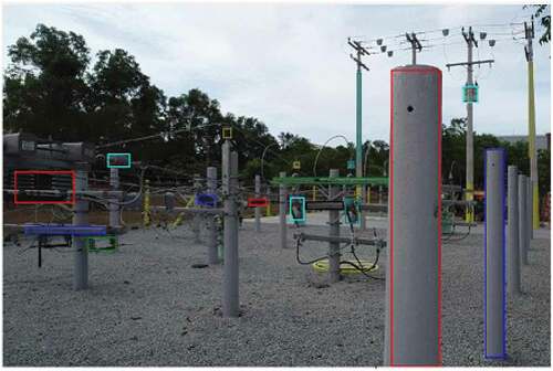
Automatic inspections generally can be done by using, for instance, videos recorded by drones. The main drawback of using drones is to modify the image’s quality due to external factors such as distance, balance, excessive vibration, or low lighting. Also, in automatic inspections, identifying each of the required objects is difficult because of their size (Liu et al. 2016), the distance between the object and the observer, and sometimes there exist intersections between them (Redmon et al. 2016), as depicted in Figure 2. For instance, the posts on the right side of the image are big objects, while the other components are much smaller and harder to identify. Therefore, the automatic identification process is challenging, requiring a robust solution to achieve better results than the regular one.

Figure 2. Electric network distribution components.

Moreover, detecting objects and/or faults is a trending subject in which deep learning has received attention from both the academy and industry. On the other hand, even though those works are efficient in detecting failures, they only identify defects in a particular power line device one at a time. Even though they sometimes can classify multiple failures, they focus on only one component. In other words, the neural networks are trained to perform the failure identification of only one kind of component. Therefore, we aim to contribute to the area in two aspects. The first one is to propose using a Convolutional Neural Network (CNN) through transfer learning (Torrey and Shavlik 2009) to identify the proper objects and at the same time classify three different defects on those components in real-time situations, even those presenting an intersection between them or very close to each other. Thus, we also aim to fill the gap of detecting defects in only one component. The second one is to build a database that can be used for training neural networks or any image-based machine learning algorithms and make it publicly available.

In this context, this paper is divided as follows: Section 2 shows some related works, and we emphasize the contributions of this work. Section 3 presents the energy lab and its components, describing why this environment is suitable for simulating fails; Section 4 introduces the used architecture, showing the YOLO pipeline, which is essential to understand why this architecture is so efficient; Section 5 shows in detail the computer experiments and used parameters; and finally, in Section 6 we show the conclusions and future work.

Related Works

In fact, some researches have been conducted to minimize the effort in detecting faults automatically. For instance, Tao et al. (2020) proposed a CNN cascade architecture in which the first network detects the insulators and the second one detects the missing caps, getting a precision of 91% and a recall of 96% using a standard insulator dataset. Huang et al. (2020) investigated a multi-class Convolutional Neural Network (CNN) to detect five defects on insulators in a dataset containing 200 images of each class. Unfortunately, Huang’s work did not show any traditional machine learning metric, using only the speed of detection and the correct rate, which were 29 seconds and 82.4, respectively.

In Qin, Zhou, and Mi (2019), the authors investigated the usage of a CNN to detect the health condition in power transformers and the location of the fault considering six types of faults. To detect the health condition, they used a CNN called LeNet-5, then they designed their CNN architecture to identify the location of failure. LeNet-5 got an accuracy of 99.3% in determining the transformer health condition, and the proposed architecture reached an accuracy of 97.02% against 93.74 of LeNet-5.

In Qu et al. (2018)’s work, the authors proposed a CNN network to detect flaws in multilevel converters. The CNN got an accuracy of 96.11% with 5% of noise, reaching an accuracy of 80.34% with 30% of noise. The CNN with no noise reached an accuracy of 98.16% and was compared against SVM (RBF and Linear) and an ANN that reached 75.17%, 86.6%, and 93.67%, respectively.

Gao et al. (2017) designed a CNN to recognize an insulator and then extract it from a scenario. First, they used a Fast R-CNN to identify the areas that potentially have an insulator. Then, the insulator is separated from the image, and the fault explosion is detected. The work detailed the CNNs based on VGG16; however, the authors do not present any performance metrics or compare their approach against other methods. The dataset is composed of 3000 images for training and only 100 images for testing.

Simple line-to-ground faults are detected in Du et al. (2018)’s work. The authors designed a CNN and compared the results with a regular artificial neural network. The CNN and ANN reached an accuracy of 96% and 93%, respectively. Liu, Zhu, and Wu (2020) implemented a simple CNN for detecting faults in Double Circuit Transmission Lines (DCTL) using three case studies with 7283, 1029, and 5145 images, obtaining an accuracy of 98.27%, 98.25%, and 98.10% on each case, respectively. Furthermore, last but not least, Mitiche et al. (2020) applied a 1-D CNN to detect faults in power lines caused by electromagnetic interference getting an accuracy of 99.4% in the proposed method, then comparing its result against RV-CNN, CV-CNN, and SVM, obtaining 86.94%, 95.37%, and 87.8%, respectively.

Specifically, our proposal investigates the use of a CNN architecture called YOLO V3 (You Only Look Once) (Redmon and Farhadi 2018), which runs over an NVIDIA GPU using a newly created dataset to get good accuracy in identifying the correct electrical component and then the most common defects in those network components. The dataset was built with images from an energy laboratory presented in the next section, a structure built for training purposes. Thus, the ambient contains many elements in the state of zero energy. The facility is localized in a neighboring region, which allowed us to manipulate the components and simulate defects, consequently creating a dataset to train our CNN. These images offered a great diversity of objects as well as lots of intersections between them.

Further, unlike the referred research that usually identifies failures in only one component, our proposal focuses on two components (cables and isolators) and detect three kinds of failures: (i) cable out of isolator, (ii) Cable out of spacer, and (iii) isolator with no ring. Furthermore, unlike some presented research that combines different approaches to identify the object and detect the failure, we use only YOLO V3 in both tasks.

The Energy Laboratory

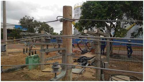
The energy lab is designed and built to provide maintenance training in the power distribution network components. The environment contains diverse structures that we can find along a railway, as depicted in Figure 3–6. As we can see, most lab components are coupled in posts with approximately 1.5 m, which was initially projected to give a hands-on experience to the employees who participate in some company training. Additionally, this short distance from the ground allowed us to take pictures to build the dataset at different distances and angles.

Figure 3. Utility structure with wooden pole.

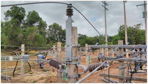
Figure 4. Power transformer structure.

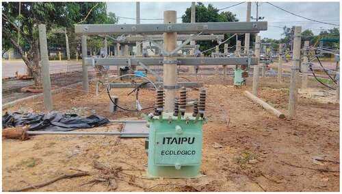
Figure 5. Section divider structure knife switch.

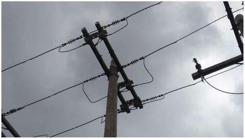
Figure 6. Deflection structure from 7º to 45º.

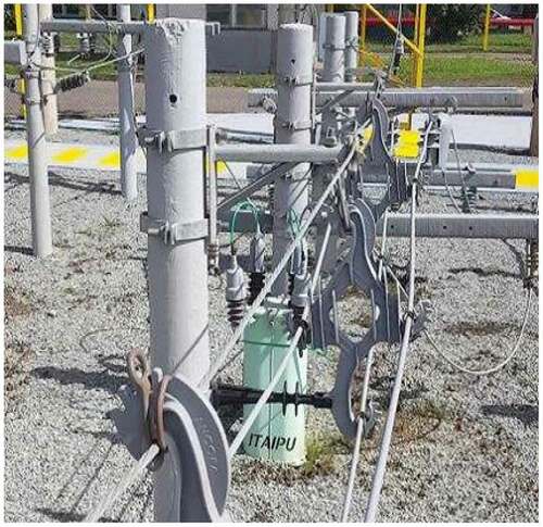
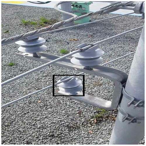
As previously mentioned, one of the challenges in identifying objects and their defects is caused by the small size of components. Also, their intersections in images represent an extra difficulty, as depicted in Figure 7–10. In other words, the simple detection of one component is more difficult because of its neighbor’s elements that can be installed in the same or near posts. Because of that, we kept in mind that pictures used to build the dataset must preserve these challenges to avoid creating a dataset that does not represent reality, leading our CNN to poor performance.

Figure 7. Example 1 of intersection.

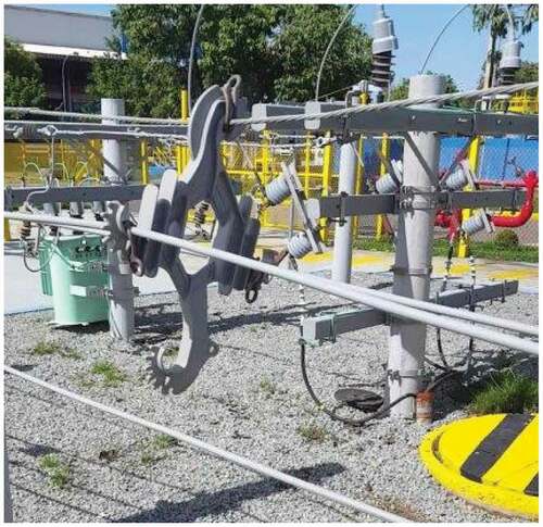
Figure 8. Example 2 of intersection.

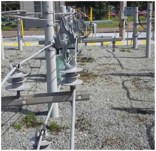
Figure 9. Example 3 of intersection.

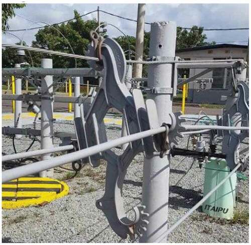
Figure 10. Example 4 of intersection.

A critical point to focus on is that, as previously mentioned, all the lab components are in a state of zero energy or no power. This condition allowed us to manipulate all objects, such as isolators, cross arms, and cables, which also allowed the simulation of many types of visible defects. In this work, as previously stated, we focus on two components (isolators and electricity cables) and three common failures: (i) cable out of isolators; (ii) cable out of spacer; and (iii) isolators with no ring.

Further, it is essential to remark that these three common defects are the most common faults we can find along with our power distribution network along the railway. Furthermore, the components are manually moved under an electrical engineer railway expert’s supervision to represent real situations found along the company’s railway. Hence, we were able to capture images to build the dataset as realistic as possible.

An important point to keep in mind is that when using a CNN to perform object detection, each training instance is devised by two components, the image itself and a file containing the annotations representing the objects to be detected. The annotation files must contain all the necessary information to make it possible to identify each object class and its position in the image. As each algorithm works with a custom format, in YOLO V3, the default format is given by: $cxywh$, in which c is the object class, x and y are the center coordinates, and w and h are the values of width and weight of the object to be detected, respectively.

The tool that we used to create the annotations relative to the defects of our dataset is the BBOX-Label-Tool (Qiu 2019). The annotations or labels created by this tool are defined by: $x_{min}$ $x_{max}$ $y_{min}$ $y_{max}$ $class\mathrm{\_}name$. Thus, it is necessary to use Equation (1)(1) $\left(\begin{array}{c}x=\frac{x_{min}+x_{max}}{2}\ast \frac{1}{w}\\ y=\frac{y_{min}+y_{max}}{2}\ast \frac{1}{h}\\ w=(x_{max}-x_{min})\ast \frac{1}{w}\\ h=(y_{max}-y_{min})\ast \frac{1}{h}\\ \hspace{0.17em}\end{array}\right.$(1) to perform a conversion to get the appropriate format.

(1) $\left(\begin{array}{c}x=\frac{x_{min}+x_{max}}{2}\ast \frac{1}{w}\\ y=\frac{y_{min}+y_{max}}{2}\ast \frac{1}{h}\\ w=(x_{max}-x_{min})\ast \frac{1}{w}\\ h=(y_{max}-y_{min})\ast \frac{1}{h}\\ \hspace{0.17em}\end{array}\right.$(1)

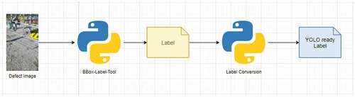
The procedure to get data ready to train the YOLO V3 is very straightforward, as we can see in Figure 11. The images were labeled using the tool BBOX-Label-Tool, so we get the set of annotations for each image. The annotations were converted into the default format expected by the YOLO V3 using a Python script to perform the transformations using the previous Equation (1)(1) $\left(\begin{array}{c}x=\frac{x_{min}+x_{max}}{2}\ast \frac{1}{w}\\ y=\frac{y_{min}+y_{max}}{2}\ast \frac{1}{h}\\ w=(x_{max}-x_{min})\ast \frac{1}{w}\\ h=(y_{max}-y_{min})\ast \frac{1}{h}\\ \hspace{0.17em}\end{array}\right.$(1) . Finally, at the end of these steps, the data preparation is complete.

Figure 11. Conversion procedure.

Samples of these defects and their pictures will be presented in Section 5. The entire dataset is available in the address https://zenodo.org/record/3972451#.X_36TuhKjIU.

The CNN Architecture: YOLO

Classic object detection methods use region proposal methods to discover possible target areas or bounding boxes in images (Girshick et al. 2014; Girshick 2015; Ren et al. 2015). Afterward, the duplicate detections are eliminated, and a classifier is used in each region to detect the possible objects. This set of procedures turns the process slow and impracticable to real-time detection. On the other hand, modern methods work differently, modeling the entire processing as a regression problem as YOLO architecture does.

YOLO (Redmon et al. 2016) is a powerful Convolutional Network that works in a straight manner. Indeed, the entire process is modeled as a fast regression process devised by two traditional neural networks steps: training and test. In the training step, we provide input images and text annotations with labels of existent objects (coordinates of boxes). In the test stage, we enter only images to obtain predictions. In both cases, the outputs of the CNN are two: the detection of the objects (bounding boxes) and the image’s prediction.

The YOLO architecture has $24$ convolutional layers and $2$ fully connected layers, as depicted in Figure 12. That disposition allows the network’s first layers to be trained with familiar objects, and its features are used in the subsequent layers.

Figure 12. Yolo architecture.

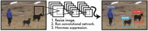
Figure 13 shows the basic procedures of the YOLO execution. The first step is to resize the image, so each image is divided into an $N\times N$ grid. Each cell of the grid is responsible for detecting objects whose center belongs to its area. Each grid cell predicts $B$ bounding boxes and confidence scores for those boxes (Redmon et al. 2016). The confidence score is defined by Equation (2)(2) $P_r(Object)\ast Io{U}_{pred}^{truth}$(2) , and the class-specific score is given by Equation (3)(3) $P_r(Clas{s}_i)\ast Io{U}_{pred}^{truth}$(3) , in which $IoU$ is the Intersection Over Union metric (Nowozin 2014). The IoU metric is important to deal with the intersection between the objects.

(2) $P_r(Object)\ast Io{U}_{pred}^{truth}$(2)

$P_r(Clas{s}_i|Object)\ast P_r(Object)\ast Io{U}_{pred}^{truth}=$

(3) $P_r(Clas{s}_i)\ast Io{U}_{pred}^{truth}$(3)

Figure 13. Yolo pipeline.

The output of the regression problem is given by an $N\times N\times (B\times 5+C)$ tensor, in which $N\times N$ is the grid cell dimension, $B$ represents how many bounding boxes each cell predicts, and $C$ is the number of classes (types of objects to be identified) in our problem. The constant $5$ in the equation refers to 5-tuple $\{x;y;w;h;s\}$, which means the central box coordinates, width, height, and confidence to each prediction, respectively.

The final step is a Non-max suppression (Neubeck and Van Gool 2006) to avoid multiple detections to the same object. This process gets more confident detections and deletes high $IoU$ with the first ones in a greedy procedure.

Computational Experiments

Setup

The CNN was implemented in C++ using the Darknet (Alexey 2020) framework. At the same time, all the tasks of the pre-processing step (image selection, labeling, renaming, resizing) were done with Python and C#. All tests were conducted in a computer with an NVIDIA GeForce© GTX 1050 with $768$ CUDA cores, $16$ GB of VRAM, and a Pentium G4560 with $2$ physical and $2$ virtual cores.

The training process is done under the pre-trained YOLO (the network was trained using pre-trained weights from Imagenet architecture (Russakovsky et al. 2015)), i.e., the first 20 layers started the training process with values capable of representing common shapes, as edges and circles.

The Database

The dataset is devised by pictures taken from different angles and distances, summing up to $708$ images stored in our dataset. From this set, $600$ images were used in the training step, while $108$ were used to test the CNN. Every picture of the dataset was also linked with an annotation file, which maintains the defective component’s coordinates in the corresponding image.

The division of defects in our dataset is presented in Table 1, while Table 2 shows the distribution in our test set. It is also important to focus on the fact that our pictures are taken from an environment with various structures that simulate a real one. Thus, each photo that contains a defective component also includes various other typical pieces of equipment.

Table 1. Distribution of dataset

Category	Quantity
Cable out of isolators	$355$
Cable out of spacer	$180$
Isolators with no ring	$172$
No defects	$93$

Table 2. Distribution of test dataset

Category	Quantity
Cable out of isolators	$42$
Cable out of spacer	$23$
Isolators with no ring	$43$

Results

The identification of the three most common defects was assigned as the YOLO task in this work. The chosen failures can be identified visually and can find these occurrences through the entire railway network. As previously mentioned, our CNN detects three main faults: cable out of isolator, cable out of spacer, and isolator with no Ring.

In this context, for a better understanding, examples of these defects are presented in Figures 14–16. It is essential to note the task’s difficulty, considering that the difference between defective and regular components is very soft, hard to detect for untrained eyes or stressed employees. The color similarity between components and background also defies the learning process and can be impossible to perform for color-blind people. Moreover, the small size of some components represents an additional difficulty.

Figure 14. Cable out of isolator.

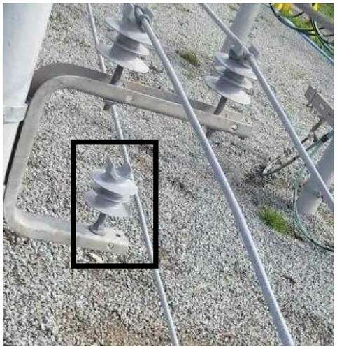
Figure 15. Cable out of spacer.

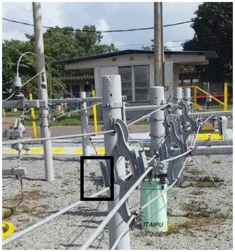
Figure 16. Isolator with no ring.

Table 3 presents the parameters of the YOLO training process. All in all, the training step was interrupted after $6000$ epochs, the update of internals filters values was executed every $64$ iterations, and the GPU processes $batch/subdivisions=1$ images per time. The parameters $Steps$ and $Scales$ mean that the learning rate was multiplied by $0.1$ after $4800$ and $5400$ iterations to smooth the learning process at the end of the training step. The other parameters, such as epochs and dataset split mode, are guided by Redmon and Farhadi (2018).

Table 3. YOLO params

Parameter	Value
Max Batches	$6000$
Batch	64
Subdivisions	$64$
Steps	[$4800$,$5400$]
Scales	[$0.1$,$0.1$]

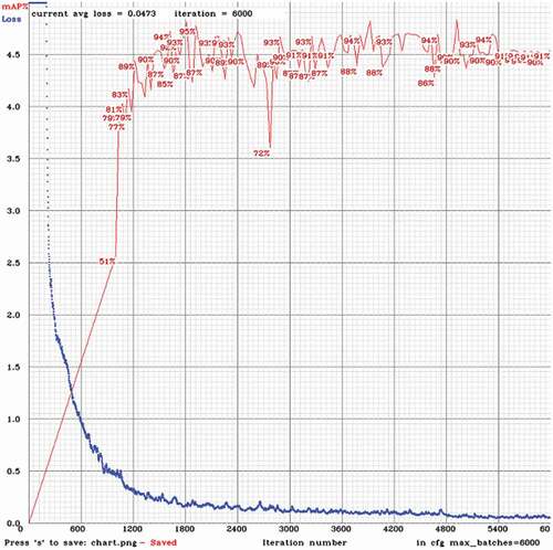
Figure 17 presents the training step as iterations go on. The blue line represents the mean square error (Wang and Bovik 2009), and the red one is the mean of the Average Precision (mAP) (Wang et al. 2013). As we can see in the referred figure, the convergence occurs in iteration $4200$ approximately. Then, considering the mAP, we can observe that the YOLO reaches stability within the interval $[3600,4500]$. Furthermore, the small values of the mAP from iteration $5400$ forward can also indicate that the YOLO network converges.

Figure 17. Iterations VS error.

To validate the model quality, the trained YOLO must be tested in new data, i.e., we used the $108$ images that were not used in the training phase. We use three model versions with weighted values of $2000$ (Version1), $4000$ (Version2), and $6000$ (Version3) iterations. This technique was used to avoid over-fitting and get the state where YOLO gets the best mAP values.

We also compare YOLO with a simpler CNN called Tiny Yolo V3 (Yu and Bouganis 2020), a state-of-the-art architecture in the field of object detection. The Tiny Yolo comprises $6$ tuples of convolution and max-pooling layers, six more convolution layers, and a final fully connected layer to predict the bounding box and confidence scores. Table 4 details the results of each model.

Table 4. YOLO results: precision, recall, IoU, and mAP

-	Version 1	Version 2	Version 3	Tiny Yolo
True Positives	95	103	100	80
False Positives	4	2	5	8
False Negatives	13	5	8	28
Precision	96%	98%	95%	91%
Recall	88%	95%	93%	74%
AP cable out spacer	89.45%	100%	90.12%	86.40%
AP cable out isolator	90.91%	90.91%	89.36%	90.68%
AP isolator without ring	97.31%	98.84%	90.68%	70.65%
Mean IoU	71.49%	76.03%	75.29%	66.87%
mAP	92.56%	96.58%	90.05%	82.57%

Analyzing all versions’ results, we can verify that Version 2 gets better performance presenting a precision of 96%, while the Tiny model presents the worst numbers. Version 2 also obtained better values regarding precision, recall, IoU, and mAP, implying that YOLO’s transfer learning configuration is the best way to identify the proper objects and, consequently, the three targeted faults.

Concerning the trained Yolo performance, the model can detect and classify at a rate of 45 FPS, which is more than enough for using the model for replacing the human inspection subject to human issues such as visual accuracy and fatigue, among others.

Discussion

There is significant effort being applied on problems on which we have to get valuable information from images, such as Object Detection (Papageorgiou and Poggio 2000) and Object Segmentation (Li et al. 2014). Considering that the Object Detection field is getting such attention, it is important to mention why modifying or improving an existent CNN model is relevant. The main point is that we always have specific problems with functional and non-functional requirements in the real world. This is an essential point about applied research.

Specifically, a power distribution network has several specific components in this work, such as isolators, electrical transformers, electrical cross arms, and spacers. So, a functional requirement is training a CNN capable of detecting such objects, which requires some research about the network architecture, which we could achieve with our strategy of applying the tests with CNN’s trained with different parameters. Another critical point is that pre-trained networks are not ready to detect objects from specific fields, so the steps of data preparation and CNN training are essential in real-world problems to obtain a good performance.

In terms of evolution, our CNN model dealt with two components and three kinds of failures, compared with previous works that dealt with only one type of defective equipment, as in Tao et al. (2020), Lei and Sui (2019), and Qin, Zhou, and Mi (2019). Another more significant point is a nonfunctional requirement, which is achieved with the use of the Darknet framework, which makes our CNN faster, reaching a mean time of $64$ ms to apply a detection in a single image, decreasing the time concerning the previous works like Tao et al. (2020), and best mAP values compared to Chen, Li, and Li (2020).

In most railroads, we have various other types of equipment (Signaling, Telecommunications, Automation, etc.) that use the power network as the main power supply. Thus, detecting those used in this work was a challenge. Also, in productive railroads (Costa et al. 2019), alternatives may exist to provide power in case of electricity failures, such as generators and batteries. In the best scenario, in which the railroad has all these elements, the operations will be working over severe constraints because alternative power supplies have their limits, such as fuel-based generators level and battery capacity. So, any process that helps in any manner to avoid failures on the main power supply can be critical to the reliability of the railway operations.

About the limitations of our investigation, it is vital to keep in mind that all the training steps must be redone if another type of failure needs to be identified. Another important consideration is that our dataset was built to simulate the current inspection activities. If some procedure is modified to imply several changes on inspection pictures, this can cause a significant worsening in the performance of our model.

Conclusion and Future Works

In this work, a CNN called YOLO was used to detect defects on power distribution network components across a railway. The model was implemented and trained using a n NVIDIA GeForce© GTX 1050 with $768$ CUDA cores. The trained model was tested using three different versions, in which version 2 presented the best results.

The model was trained using a dataset generated in the energy laboratory, which allowed us to simulate defects in interest faults. The best model (version 2) reached a precision of $98\mathrm{\%}$ and an mAP of $96.58\mathrm{\%}$ in the test step. These are promising results, considering that:

• Most of the components have a small dimension in comparison with the total area of the image;

• The images of components in a power distribution network usually present a short distance of other components;

• The difference between a defective and a regular component is very smooth;

• The inspection images have to deal with noise because of the image background.

All in all, the YOLO architecture showed a good relationship between detection velocity and precision, considering that the architecture can make detections and classification at 45 fps when running in a GPU and got $96.58\mathrm{\%}$ of mAP on the test phase.

Future work consists of testing modifications in the current architecture using meta-heuristics, training the YOLO model using more fault categories, and testing the network in embedded platforms such as NVIDIA Jetson Nano boards.

Disclosure statement

No potential conflict of interest was reported by the author(s).

References

- Alexey. 2020. Yolo-v3 and yolo-v2 for windows and linux. Accessed March 29, 2020. https://github.com/AlexeyAB/darknet#how-to-train-to-detect-your-custom-objects.
- Chen,W., Y.Li, and C. Li. 2020. A visual detection method for foreign objects in power lines based on mask r-cnn. International Journal of Ambient Computing and Intelligence (IJACI) 11 (1):34–47. doi:https://doi.org/10.4018/IJACI.2020010102.
- Costa, J. P. A., O. A. C. Cortes, V. B. S. N. de Oliveira, and A.C. F. da Silva. 2019. Deep neural networks applied to the dynamic helper system in a gpgpu. In International Conference on Artificial Intelligence and Soft Computing, Zakopane, Poland, 29–38 doi:https://doi.org/10.1007/978-3-030-20912-4_3. Springer.
- Du, Y., Q.Shao, Y. Liu, G. Sheng, and X. Jiang. 2018 Detection of Single Line-to-Ground Fault Using Convolutional Neural Network and Task Decomposition Framework in Distribution Systems International Conference on Condition Monitoring and Diagnosis (CMD) Perth, WA, Australia (IEEE). (), 1–4 doi:https://doi.org/10.1109/CMD.2018.8535600.
- Gao, F., J.Wang, Z.Kong, J. Wu, N.Feng, S.Wang, P.Hu, Z. Li, H.Huang, and J.Li. 2017. Recognition of insulator explosion based on deep learning. In 14th International Computer Conference on Wavelet Active Media Technology and Information Processing (ICCWAMTIP), Chengdu, China (IEEE), 79–82 doi:https://doi.org/10.1109/ICCWAMTIP.2017.8301453.
- Girshick,R. 2015. Fast R-CNN. In Proceedings of the IEEE International Conference on Computer Vision, Santiago, Chile (IEEE), 1440–1448 doi:https://doi.org/10.1109/ICCV.2015.169.
- Girshick, R., J. Donahue, T. Darrell, and J. Malik 2014). Rich feature hierarchies for accurate object detection and semantic segmentation. In Proceedings of the IEEE Conference on Computer Vision and Pattern Recognition, Colombus, OH, USA (IEEE), 580–587 doi:https://doi.org/10.1109/CVPR.2014.81.
- Huang,X., E.Shang, J. Xue, H. Ding, and P. Li. 2020. A multi-feature fusion-based deep learning for insulator image identification and fault detection. In 2020 IEEE 4th Information Technology, Networking, Electronic and Automation Control Conference (ITNEC), Chongqing, China, (IEEE), 1957–1960 doi:https://doi.org/10.1109/ITNEC48623.2020.9085037.
- Lei, X., and Z.Sui. 2019. Intelligent fault detection of high voltage line based on the faster r-cnn. Measurement 138:379–385. doi:https://doi.org/10.1016/j.measurement.2019.01.072.
- Li, Y., X.Hou, C.Koch, J. M. Rehg, and A.L Yuille. 2014. The secrets of salient object segmentation. In Proceedings of the IEEE conference on computer vision and pattern recognition, Colombus, OH, USA (IEEE), 280–287 doi:https://doi.org/10.1109/CVPR.2014.43.
- Liu,W., D.Anguelov, D. Erhan, C. Szegedy, S. Reed, C.-Y.Fu, and A. C. Berg. 2016. SSD: Single shot multibox detector. In European conference on computer vision, Amsterdam, The Netherlands, 21–37 doi:https://doi.org/10.1007/978-3-319-46448-0_2. Springer.
- Liu, Y., Y. Zhu, and K. Wu. 2020. Cnn-based fault phase identification method of double circuit transmission lines. Electric Power Components and Systems 48 (8):833–843. doi:https://doi.org/10.1080/15325008.2020.1821836.
- Mitiche, I., A.Nesbitt, S. Conner, P. Boreham, and G. Morison. 2020. 1d-cnn based real-time fault detection system for power asset diagnostics. IET Generation, Transmission & Distribution 14 (24):5766–5773. doi:https://doi.org/10.1049/iet-gtd.2020.0773.
- Neubeck, A., and L. Van Gool. 2006. Efficient non-maximum suppression. In 18th International Conference on Pattern Recognition (ICPR’06), Hong Kong, China, vol. 3, 850–855 doi:https://doi.org/10.1109/ICPR.2006.479. IEEE.
- Nowozin, S. 2014. Optimal decisions from probabilistic models: The intersection-over-union case. In Proceedings of the IEEE Conference on Computer Vision and Pattern Recognition, Columbus, OH, USA (IEEE), 548–555 doi:https://doi.org/10.1109/CVPR.2014.77.
- Papageorgiou, C., and T. Poggio. 2000. A trainable system for object detection. International Journal of Computer Vision 38 (1):15–33. doi:https://doi.org/10.1023/A:1008162616689.
- Qin, J., B.Zhou, and Z. Mi. 2019. Research of fault diagnosis and location of power transformer based on convolutional neural network. In 2019 IEEE Innovative Smart Grid Technologies - Asia (ISGT Asia), Chengdu, China (IEEE), 3589–3594 doi:https://doi.org/10.1109/ISGT-Asia.2019.8881485.
- Qiu, S. 2019. Bbox-label-tool.
- Qu, X., B. Duan, Q. Yin, M.Shen, and Y.Yan. 2018. Deep convolution neural network based fault detection and identification for modular multilevel converters. In IEEE Power Energy Society General Meeting (PESGM), Portland, OR, USA (IEEE), 1–5 doi:https://doi.org/10.1109/PESGM.2018.8586661.
- Redmon,J., and A.Farhadi. 2018. Yolov3: An incremental improvement. arXiv preprint arXiv:1804.02767.
- Redmon, J., S. Divvala, R.Girshick, and A. Farhadi. 2016. You only look once: Unified, real-time object detection. In Proceedings of the IEEE conference on computer vision and pattern recognition, Las Vegas, NV, USA (IEEE), 779–788 doi:https://doi.org/10.1109/CVPR.2016.91.
- Ren, S., K. He, R. Girshick, and J. Sun. 2015 Faster R-CNN: Towards Real-Time Object Detection with Region Proposal Networks .In Advances in Neural Information Processing Systems Montreal, Canada , 91–99.
- Russakovsky, O., J. Deng, H. Su, J. Krause, S. Satheesh, S. Ma, Z. Huang, A. Karpathy, A. Khosla, and M. Bernstein, et al. 2015. Imagenet large scale visual recognition challenge. International Journal of Computer Vision. 115(3):211–252. doi:https://doi.org/10.1007/s11263-015-0816-y.
- Tao, X., D. Zhang, Z. Wang, X. Liu, H. Zhang, and D.Xu. 2020. Detection of power line insulator defects using aerial images analyzed with convolutional neural networks. IEEE Transactions on Systems, Man, and Cybernetics: Systems 50 (4):1486–1498. doi:https://doi.org/10.1109/TSMC.2018.2871750.
- Torrey, L., and J. Shavlik. 2009. Transfer learning. In Handbook of research on machine learning applications and trends: Algorithms, methods and techniques, ed. E. S. Olivas, J. D. M. Guerrero, M.M. Sober, J. R. M. Benedito, and A. J. S. Lopez, 242–64. Hershey, New York: Information Science Reference. chapter 11.
- Wang,X., M. Yang, S. Zhu, and Y. Lin. 2013. Regionlets for generic object detection. In Proceedings of the IEEE international conference on computer vision, Sydney, NSW, Australia (IEEE), 17–24 doi:https://doi.org/10.1109/ICCV.2013.10.
- Wang, Z., and A. C. Bovik. 2009. Mean squared error: Love it or leave it? A new look at signal fidelity measures. IEEE Signal Processing Magazine 26 (1):98–117. doi:https://doi.org/10.1109/MSP.2008.930649.
- Yu, Z., and C.-S. Bouganis. 2020. A parameterisable fpga-tailored architecture for yolov3-tiny. In Applied reconfigurable computing. Architectures, tools, and applications, ed. F. Rincón, J. Barba, H.K.H. So, P. Diniz, and J. Caba, 330–44. Cham: Springer International Publishing.