Ensemble Classifier for Stock Trading Recommendation

ABSTRACT

This paper presents a heterogeneous ensemble classifier for price trend prediction of a stock, in which the prediction results are subsequently used in trading recommendation. The proposed ensemble model is based on Support vector machine, Artificial neural networks, Random forest, Extreme gradient boosting, and Light gradient boosting machine. A feature selection is performed to choose an optimal set of 45 technical indicators as input attributes of the model. Each base classifier is executed with an extensive hyperparameter tuning to improve performance. The prediction results from five base classifiers are aggregated through a modified majority voting among three classifiers with the highest accuracies, to obtain final prediction result. The performance of proposed ensemble classifier is evaluated using daily historical prices of 20 stocks from Stock Exchange of Thailand, with 3 overlapping datasets of 5-year intervals during 2014–2020 for different market conditions. The experimental results show that the proposed ensemble classifier clearly outperforms buy-and-hold strategy, individual base classifiers, and the ensemble with straightforward majority voting in terms of both trading return and Sharpe ratio.

Introduction

Stock trend prediction is very valuable for investment management. Accurate prediction makes it possible for investors to decide a proper moment to buy or sell a stock, to achieve the goal to beat the market and make profits (Ding and Qin 2020). However, stock trend prediction is really challenging due to the high volatility in the stock market. The trend prediction in stock market has drawn a lot of research attention for many decades using both statistical and computing approaches including artificial intelligence. Recent approaches focus more on machine learning with both regression and classification techniques. Regression techniques aim to predict the future value of the stock price (Wang et al. 2011), while classification techniques aim to predict the trend of stock price movement (Deng et al. 2021; Kim and Han 2016; Nobre and Neves 2019; Olson and Mossman 2003; Zhang et al. 2018, 2021).

Broadly speaking, there are two approaches in analyzing financial market: fundamental analysis and technical analysis. Fundamental analysis studies the economic factors and financial factors of the firm to predict its price or trend. Technical analysis approach believes that the historical data of the firm’s prices can be mathematically analyzed for predicting the trend. Technical analysis has been widely used for short-term trading, in a range of weeks to hours (Hu et al. 2015; Lorenzo 2013).

This work aims to apply five well-known classification algorithms, namely, support vector machine, artificial neural network, random forest, extreme gradient boosting (or XGBoost), and light gradient boosting machine (or LightGBM) for trend prediction. The aim is to propose a heterogeneous ensemble classifier from such five base algorithms to predict trend of stock price for trading recommendation. Performance of the algorithms will be evaluated with the investment returns and risks from trading simulation using the predicted trend results.

Specifically, in the first step, the classifiers are trained to build a trend prediction model from a daily dataset. The experiment uses publicly available data of open, high, low, close, and volume of stock prices. These raw data are used to compute a set of technical indicators which are widely used by technical analysts. The computed technical indicators are fed into the process of building the prediction models. However, up to now, there is no known set of technical indicators most suitable for a dataset. A feature (or attribute) selection method is adopted in the data preprocessing to automatically choose the optimal technical indicators as model inputs. The models are used for predicting daily trends of the corresponding testing (or unseen) data, which will further be used for trading simulation in the second step. Moreover, choosing the optimal classification algorithm and its hyperparameter for a given data often requires expertise and amount of effort (Elshawi, Maher, and Sakr 2019). Hyperparameters are parameters of the algorithm itself that need to be set to suitable values to obtain good performance for a given data. Most of the time they are left to using default values, which unfortunately often lead to performance much lower than of the hyperparameter tuning. Thus in this work, performance and optimum parameters for a given algorithm are explored by using grid search method.

Most works on classification algorithm usually compare the performance with common classification metrics such as accuracy. However, there are usually inconsistencies between model’s performance and profitability. Classification metrics like accuracy do not take into account the profit information. The model with optimal metric value cannot guarantee the optimal profitability (Guang and Wang 2019; Teixeira and De Oliveira 2010). Therefore, an ensemble method is used to aggregate the results from base classifiers to arrive at a collaborated decision (Tsai et al. 2011).

In the second step, the predicted trend results are employed in a trading recommendation system – that is to buy, to sell, or to do nothing if the predicted trend is positive, negative, or very small, respectively. The investment returns from trading simulation with the testing data are calculated. Performance of the proposed model is evaluated using trading return and Sharpe ratio. Sharpe ratio is a measure of risk-adjusted return, describing how much excess return received for the volatility (or risk) of holding a riskier asset (Sharpe 1994). The returns and Sharpe ratios are to be compared with the trading using prediction results from individual classifier as well as with two other cases – one is the buy and hold (B&H) and the other is if we know the future (KF).

This research contributes to (1) construct a heterogeneous ensemble classifier that aggregates results from different base classifiers, each of which using an extensive hyperparameter tuning. Inputs of each base classifier are various commonly used technical indicators automatically chosen with a feature selection method. In addition, we also (2) propose a trading recommendation system based on the trend prediction result from the ensemble classifier.

The remaining of this article is organized as following. The next section reviews related literature about technical analysis and financial trend prediction using classification algorithms. Then the proposed ensemble classifier will be described, and its performance is evaluated and discussed. Finally, the last section concludes this work with its limitations and future works.

Related Works

Technical Analysis and Indicators

In financial markets, technical analysis develops technical indicators and several charts from historical prices and uses them to predict trends or provide trading signals (Hu et al. 2015; Lorenzo 2013). There are hundreds of technical indicators developed for the past decades, but the most popular ones are limited to fewer than 20 of them. Technical indicators can be classified into four types – trend, momentum, volume, and volatility (Hu et al. 2015). First, trend indicators tell us which direction the price is moving in, upward, downward, or sideway – there is no trend. Simple Moving Average (SMA) and Exponential Moving Average (EMA) are the most popular examples of trend indicators. Second, momentum indicators evaluate the velocity of price change and judge whether a reversal is about to happen. Common momentum indicators are Moving Average Convergence Divergence (MACD), Stochastic Oscillator (%K and %D), and Relative Strength Index (RSI). Third, volume indicators measure the strength of a trend or confirm a trading direction based on some form of averaged volume traded. A popular volume indicator is On Balance Volume (OBV). Fourth, volatility indicator measures the range of price movement and can be used to identify level of support and resistance. Common volatility indicator includes Bollinger Band (BB) (Hu et al. 2015; Lorenzo 2013).

Trend Prediction with Classification Techniques

Classification algorithms try to classify data into a given number of classes. Classification algorithms can be employed straightforwardly for prediction of the trend or direction of stock returns into positive or negative, for example. During the past two decades, the widely used classification algorithms with proved performance are support vector machine, artificial neural networks, and random forest. More recently, tree-ensembled methods have significantly improved performance and are increasingly accepted as state-of-the-art. Among them are extreme gradient boosting (or XGBoost) and light gradient boosting machine (or LightGBM).

Support vector machine (SVM) is a statistical learning technique that constructs a hyperplane as the decision surface that maximized the margin of separation of different classes (Cortes and Vapnik 1995). Given a set of training examples (x_i,y_i), i = 1, 2, …, l. Where x_i ∈ Rⁿ and y_i ∈{-1, 1} is the label of x_i, a standard SVM model is formulated as $\underset{\mathrm{w},\mathrm{b}}{\mathrm{m}\mathrm{i}\mathrm{n}}\frac{1}{2}\mathrm{w}{ }^2$ s.t. y_i (<w, x_i> +b) ≥ 1, i = 1, 2, …, l; where w is the normal vector of hyperplane, b is a bias value, and <p, q> is the inner product of vectors p and q. The goal of SVM to maximize the margin of separation of different classes is to minimize $\mathrm{w}{ }^2/2$.

SVM is one of the early successful algorithms for trend prediction. Huang, Nakamori, and Wang (2005) investigated the predictability of weekly movement direction of NIKKEI 225 index with SVM. Their experiment results showed SVM outperformed Linear Discriminant Analysis, Quadratic Discriminant Analysis and Elman Backpropagation Neural Networks. Ni, Ni, and Gao (2011) proposed an SVM model with fractal feature selection of 19 technical indicators and a grid search method using fivefold cross validation to predict direction of Shanghai stock index. Luo et al. (2017) improved their integrated piecewise linear representation and weighted support vector machine (PLR-WSVM) for trading 20 China stock. Their SVM model with relative technical indicators and automatic threshold has improved performance in classification of turning points and ordinary points for making more profitable trading decision.

Artificial Neural Network (ANN) is biologically inspired computing models which can be used to find knowledge, patterns, or models from a large amount of data (Bose and Liang 1996). ANN consists of connected computational units or nodes, called neurons, arranged in several layers. Each neuron combines its inputs, each of which is multiplied with a weight, and then passes it through an activation function, which can be a linear or nonlinear filter (such as sigmoid or tanh functions). Then the neuron sends its output to other neurons or to be output of the network. The interconnection of all neurons forms different types of architectures designed for various functions. The most widely used architecture is called feed-forward multilayer perceptron (MLP) which generally used back-propagation (BP) learning algorithm to adjust its weights for supervised learning. BP works in an iteration of three steps. The first step is propagating inputs forward through the hidden layers to the output nodes. The second step is to propagate the errors backward through the network starting from output layer. And the final step is to update the weight and biases using approximate steepest descent rule. Such three steps repeat until reaching the maximum iterations allowed with the aim to minimize the errors of output during the training.

ANN has demonstrated promising results in predictions of stock price trends during the past two decades. Olson and Mossman (2003) compared the forecasts of one-year-ahead Canadian stock returns using ANN, logistic regression and ordinary least squares. The results demonstrated that ANN outperformed the other two algorithms. O’Connor and Madden (2006) included some external indicators, such as currency exchange rates, in predicting movements in the Dow Jones Industrial Average index using ANN models. Kara, Boyacioglu, and Baykan (2011) predicted the direction of stock price movement in the Istanbul Stock Exchange using ANN and SVM with ten technical indicators as inputs. The empirical results demonstrated that their ANN model performed better than SVM model. Chen, Leung, and Daouk (2003) applied probabilistic neural network to predict the direction of return on Taiwan Stock Exchange and found that their model demonstrated a more predictive power than generalized methods of moments with Kalman filter and random walk.

Random forest (RF) is an efficient learning algorithm for classification that is constructed from many unpruned decision trees (DT) from random subsets of features using bootstrapped training data (Breiman 2001). The accuracy (or probability of correct prediction) of a single tree may not be high, but the combination of many trees, forming the forest, results in a higher accuracy. Construction of RF mainly includes two stages. The first stage is the generation of forest, in which the training samples are divided into many samples at random, construct CART (Classification and Regression Tree) decision trees. When creating partitions to a feature, the goodness of a partition is measured by purity. If a partition is pure, for each sub-branch of this node, its instances belong to the same class (Zhang et al. 2018). The second stage is to determine the classification results from the forest. For a classification task, the result combination can be as simple as majority voting (Breiman 2001). This ensemble method enhances the accuracy of RF over the single DT, while the problem of overfitting is controlled simultaneously.

Zhang et al. (2018) proposed a model using random forests, imbalance learning, feature selection and clipping for prediction of both stock price movement and its interval of growth (or decline) rate. Using more than 70 technical indicators as inputs, the model classified prediction targets into 4 classes: up, down, flat, and unknown. The model was evaluated using more than 400 stocks in Shenzhen Market and the results revealed that it outperforms ANN, SVM and K-Nearest Neighbors in terms of accuracy and return per trade. Thakur and Kumar (2018) applied RF to discover the optimal feature subset from a large set of technical indicators from daily data of five index futures for trading. Kim and Han (2016) predicted the direction of movement of stock index using a modified random forest where bootstrap also determined the weights based on the degree of Korea composite stock index change. The experimental results confirmed that their enhanced random forest outperformed the classical random forest with statistical significance.

XGBoost (eXtreme Gradient Boosting) is an efficient ensemble machine learning system, developed by Chen and Guestrin in 2016 (Chen and Guestrin 2016). XGBoost improves Friedman’s gradient boosting technique (Friedman 2001) that employs DT as base learners to fit the training data and use a tree ensemble model to sum the score of each tree to get the final prediction. The objective function of the XGBoost is to combine the standard penalty term with the loss function term to obtain the optimal solution. XGBoost uses regularization to control the flexibility of the learning task and to obtain models that generalize better to unseen data. In addition, its loss function is optimized by second-order Taylor expansion to help avoid overfitting.

Due to its efficiency and fast operation, XGBoost has been widely applied in financial applications. For example, Nobre and Neves (2019) applied XGBoost for binary classifier for predicting trend of five different financial time series for trading simulation. Hyperparameters of their XGBoost are optimized with multiobjective genetic algorithm. The empirical results showed that their system can outperform the Buy and Hold (B&H) strategy in three of the five analyzed financial markets. Chen et al. (2021) proposed a novel portfolio construction approach based on XGBoost for stock price prediction. Hyperparameters of XGBoost are optimized using an improved firefly algorithm. Their experiment demonstrated that this approach yielded the best results in terms of returns and risks. Deng et al. (2021) proposed a novel hybrid method of XGBoost with bagging and regrouping particle swarm optimization (RPSO) for direction forecasting of a high-frequency future trading simulation. A bagging method is incorporated to solve overfitting problem while the RPSO is for optimizing hyperparameters of XGBoost. The empirical results reveal that their hybrid model outperforms SVM, RF and buy-and-hold with many evaluation criteria. Yun, Yoon, and Won (2021) proposed a hybrid model of XGBoost and genetic algorithm with an extensive feature engineering process on more than 60 technical indicators for stock market predictions. Their hybrid model can outperform LSTM models in terms of both performance and interpretability.

LightGBM is also a gradient learning tree-based framework with boosting technique to integrate results from weak learners to enhance performance (Ke, Menget al. 2017). Its main difference from the XGBoost model is that it uses Gradient-based One Side Sampling (GOSS) and automated feature selection with Exclusive Feature Bundling (EFB). With GOSS, LightGBM uses histogram algorithm to discretize continuous floating-point eigenvalues into many bins. Histogram algorithm does not need extra storage of presorted results and thus greatly reduces memory consumption without scarifying the accuracy of the model. EFB reduces the optimal bundling of exclusive features to a graph coloring problem and solves it by a greedy algorithm with a constant approximation ratio. Both GOSS and EFB makes LightGBM lighter and efficient. In addition, LightGBM uses leaf-wise tree growth strategy, which effectively finds the leaves with the highest branching gain each time from all the leaves, and then goes through the branching cycle. Therefore, it can reduce more errors and obtain better precision with the same number of times of segmentation. A maximum depth limit is set to prevent overfitting while ensuring high efficiency.

With high prediction accuracy, fast computational speed and preventing of overfitting, LightGBM has been widely applied in many fields. Zhang et al. recently propose a smart contract Ponzi scheme identification method based on the improved LightGBM algorithm (Zhang et al. 2021). Experiments are conducted on the real Ethereum data set which is imbalanced. The results prove that their proposed method has highly improved accuracy, F-score and the area under the receiver operating characteristics curve (AUC) metrics compared with XGBoost and RF. Slezak, Butler, and Akbilgic (2021) preoperatively predict risk of postoperative readmission for total joint replacement surgery among older persons. The dataset has 22 predictor variables and is highly imbalance. The experimental results indicate that LGBM outperforms XGboost, RF, and Logistic Regression using AUC obtained in the holdout data. Oram et al. (2021) proposed a LGBM-based phishing e-mail detection model using phisher websites’ features of mimic URLs. Their experimental result show that LGBM outperforms XGBoost, AdaBoost, RF, and many other classical classification algorithms in terms of accuracy and F1 score.

Issues Related to Classification

Unfortunately, using machine learning algorithms is not an easy task. There are three common issues for thorough considerations: (i) feature selection, (ii) hyperparameter tuning, and (iii) no free lunch theorem and ensemble.

Feature Selection

First, one major question is how to choose a proper set of attributes, called features, to be inputs of the model. Feature selection methods become an important step of data preprocessing for the classification algorithm. Feature selection approaches fall into three categories: filter based, wrapper based, and embedded (Li et al. 2018; Xue et al. 2016).

1. Filter-based methods uses statistical data dependency techniques to find the subset of features.

2. Wrapper-based methods evaluate candidate subsets by a learning algorithm and thus itself requires parameter tuning.

3. Embedded methods incorporate knowledge about the specific structure of the algorithm while selecting features in the training process (Cai et al. 2018). Thus, they are generally applicable to only specific classification algorithms (Nguyen, Xue, and Zhang 2020).

Both wrapper-based and embedded methods are computing intensive. The filter-based approach is usually considered efficient in most cases since it does not involve any learning process, and is chosen for use in this work.

Hyperparameter Tuning

Second, building an effective classification model is a complex and time-consuming process that involves tuning its hyperparameters (Nguyen, Xue, and Zhang 2020; Yang and Shami 2020). Tuning hyperparameters is considered a key component of building an effective machine learning model, especially for tree-based or neural-based models like RF and ANN, which have many hyperparameters. Accurate results for ANN highly depend on a careful selection of its hyperparameters such as number of hidden layers, number of nodes in each layer the learning rate, input variables, etc. (Hussain et al. 2008). Unfortunately, manual tuning of hyperparameters not only requires expertise but also is prone to getting lower performance.

Grid search is one of the most commonly used methods to explore hyperparameter configuration space. It involves exhaustively search that evaluates all the hyperparameter combinations given to a grid of configurations (Nguyen, Xue, and Zhang 2020; Yang and Shami 2020). In this work, we use grid search for hyperparameter tuning of all selected classification algorithms for an optimal performance. Although this approach is time consuming, this work does not aim to run in a real-time environment.

No Free Lunch Theorem and Ensemble

Third, there are several algorithms available for a given problem class and there is no definite guideline to select the algorithm best fit the problem. According to well-known No Free Lunch theorem (Wolpert and Macready 1997), no single method may outperform others in all situations. Classification algorithms are not exceptions. No one can foretell which algorithm will outperform in all tested datasets. Ensemble learning is an approach to overcome this challenge by combining multiple classifiers, forming committee to improve prediction, and is believed to perform better than single classifiers. Ensemble techniques have been applied in several application domains including energy and financial prediction, which can be briefly reviewed as following.

Khairalla et al. (2018) proposed a stacking multilearning ensemble model with support vector regression, ANN, and linear regression, for prediction of oil consumption. The experimental results demonstrated that their ensemble model outperforms classical models for both 1-ahead and 10-ahead horizon prediction, in terms of error rate, similarity, and directional accuracy. Nti, Adekoya, and Weyori (2020a) performed an extensive comparative analysis of different ensemble methods such as bagging, boosting, stacking, and blending for stock market prediction. They constructed 25 different ensemble regressors and classifiers using DT, MLP, and SVM for stock indexes from four countries. The obtained result revealed that the stacking technique outperformed boosting, bagging, blending, and simple maximum in stock market prediction. Nti, Adekoya, and Weyori (2020b) proposed a homogeneous ensemble classifier based on Genetic Algorithm for feature-selection and optimization of SVM parameters for predicting 10-day-ahead price movement on the Ghana stock exchange. They employed a simple majority voting ensemble method to combine results from 15 different SVM models using 14 technical indicators as inputs. Their empirical results showed that their ensemble model provided a higher prediction accuracy of stock price movement as compared with DT, RF, and NN. Ampomah, Qin, and Nyame (2020) compared the effectiveness of different tree-based ensemble models including RF, XGBoost, Bagging Classifier, AdaBoost, Extra Trees Classifier, and Voting Classifier in forecasting the direction of stock price movement. Eight different stock data from three stock exchanges (NYSE, NASDAQ, and NSE) were used for the study. They employed principal component analysis to do feature selection of 45 inputs including 40 technical indicators. The empirical results revealed that Extra Trees classifier outperformed the other models in all the rankings.

In general, ensemble methods can be divided into homogeneous and heterogeneous approaches (Polikar 2006). In homogeneous ensemble, all base classifiers are from the same family (e.g. tree-based), whereas in heterogeneous ensemble, we construct the ensemble model from the classifiers having different learning strategies. The heterogeneous classifier ensembles offer slightly better performance than the homogeneous ones (Tsai et al. 2011). The common ensemble strategies are majority voting, bagging (Breiman 1996) and boosting (Breiman 2001). However, it might be inconclusive to identify which strategy clearly outperforms the others. This work employs an ensemble classification model that works on the modified majority voting of results of five classifiers.

The Proposed Model

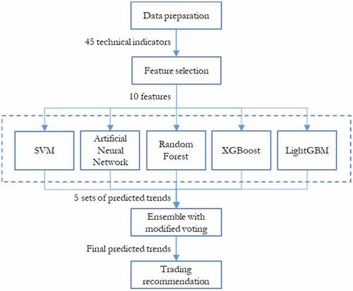
This work proposes an ensemble classifier built from SVM, RF, ANN, XGBoost, and LightGBM to develop trend prediction models for stock prices. The trend prediction results will be used to recommend trading decisions (to long, to short, or to do nothing) in a trading simulation using the testing data. The returns obtained from the simulation will be compared. This work is developed using Python 3.8 platform on Windows 10 and 16-core Intel Core i9 processor running 2.50 GHz. The whole process of trend classification for trading is shown in Figure 1. It includes five stages of process including data collection and preparation, feature selection, base classification, ensemble with majority voting approach, and trading simulation as explained below.

Figure 1. Process.

Data Collection and Preparation

The prediction in this work is based on technical analysis approach. Inputs to the process are daily open, high, low, close and volume data downloaded from web finance.yahoo.com. The input data are used for computing 45 technical indicators listed in Table 1. All these indicators, forming attribute, or feature set of the classifiers, are commonly used by the technical practitioners in stock markets. Their descriptions and formulas can be found in Hu et al. (2015) and Lorenzo (2013). Some of them e.g. RSI, DISP, and ROC use varying periods to deal with uncertainty. Then every feature is normalized to range [0, 1] before further processing.

Table 1. Technical indicators used

Indicator	Description	Number of indicator(s)
RSI10, RSI15, RSI20, RSI25	Relative Strength Index (10, 15, 20, and 25 days)	4
SLOWK, SLOWD	Stochastic Oscillators (%K, %D)	2
ADX10, ADX20	Average Directional Movement Index (10-day and 20-day)	2
BBAND10, BBAND20, BBAND30	Bollinger Band (10-day, 20-day, 30-day)	3
DISP1, DISP2, DISP5, DISP10, DISP20, DISP50, DISP100	Disparity n = 1, 2, 5, 10, 20, 50, 100 days	7
AROONOSC	Aroon Oscillator (14-day)	1
CCI14, CCI28	Commodity Channel Index (14-day and 28-day)	2
CMO14	Chande Momentum Oscillator (14-day)	1
DMI14	Directional Movement Index (14-day)	1
MACD(12, 26)	Moving Average Convergence and Divergence	3
MFI10, MFI14, MFI20	Money Flow Index (10-day, 14-day, 20-day)	3
PPO12:26, PPO9:20	Percentage Price Oscillator (12–26-day, 9–20-day)	2
ROC5, ROC10, ROC20, ROC40, ROC80	Rate of Change (5-day, 10-day, 20-day, 40-day, 80-day)	5
TRIX30	Triple Smooth EMA (30-day)	1
WILLR10, WILLR15, WILLR20	William %R (10-day, 15-day, 20-day)	3
ADOSC(3, 10)	Accumulation/Distribution Oscillator (3–10-day)	1
OBV	On Balance Volume	1
NATR10, NATR15, NATR20	Normalized Average True Range (10-day, 15-day, 20-day)	3

Feature Selection

However, some features might be redundant features providing similar information for the learning task while others might be irrelevant providing misleading information that deteriorates the learning performance. A filter-based approach feature selection is chosen in this work to remove redundant or irrelevant features. The filter-based methods evaluate feature subsets using their intrinsic properties (Xue et al. 2016) such as correlation, information, distance, etc. In this work, we use a univariate filter-based method that removes all but the highest Chi-square scoring features.

Base Classification

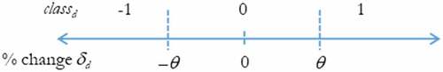
The model aims to predict the trend of closing price at day d + 2 (close_{d + 2}) compared to the opening price on the next day d + 1 (open_{d + 1}). Specifically, output of the model, called class_d ∈{-1, 0, 1}, represents direction of δ_d or percentage change of day d as of the following equation:

(1) $\delta d=100\hspace{0.17em}\frac{clos{e}_{d+2}-ope{n}_{d+1}}{ope{n}_{d+1}}$(1)

where $\mathrm{c}\mathrm{l}\mathrm{o}\mathrm{s}{\mathrm{e}}_{\mathrm{d}}$ and $\mathrm{o}\mathrm{p}\mathrm{e}{\mathrm{n}}_{\mathrm{d}}$ are the closing price and opening price of day d. The value of class_d is determined by comparing δ_d with a decision threshold θ as in Figure 2. That is class_d is 0 if the percentage change δ_d is between -θ and θ. Otherwise class_d will be −1 or 1 if δ_d is less than -θ or greater than θ respectively. The sign of the class value indicates short-term direction, i.e. positive is uptrend and negative is downtrend. Class 0 implies that the change is so small that the potential profit is difficult to beat transaction fee.

Figure 2. Determining class_d from δ_d.

Hyperparameter Tuning

As discussed in previous section, performance of any classifiers highly depends on its hyperparameter setting. Grid search method is employed in this work to explore hyperparameter configuration space. It exhaustively evaluates all the hyperparameter combinations (Yang and Shami 2020) of all five base classifiers as following.

SVM

kernel[‘rbf,’ ‘poly’]

C[0.01, 0.1, 1, 10, 100]

gamma[1, 0.1, 0.01, 0.001]

ANN

solver[‘adam,’ ‘sgd’]

activation[‘tanh,’ ‘relu’]

learning_rate[‘invscaling,’ ‘adaptive’]

learning_rate_init[0.01, 0.001]

hidden_layer_sizes[(20,), (40,), (60,), (40, 40)]

RF

criterion[‘gini,’ ‘entropy’]

n_estimators[100, 400]

max_depth[5, 9, 13]

min_samples_split[2, 6]min_samples_leaf [1, 5]

XGBoost

max_depth[4, 8]

learning_rate[0.0005, 0.01]gamma [0.1, 1.0]

subsample[1.0, 0.7]

min_child_weight[0.02, 1, 5.]

LightGBM

max_depth[5, 10, 15]

learning_rate[0.005, 0.05]num_leaves [20, 40, 60]

max_bin[100, 200, 300]

Performance of SVM depends upon the selected kernel function, regularization parameter C, and gamma. The kernel function defines the hyperplane used for separating data into different classes. Regularization parameter controls the trades off between error minimization and margin maximization. The parameter gamma specifies the desired curvature for the radial basis function kernel.

Performance and complexity of an ANN mainly depend upon the number of hidden layers and the number of nodes in each layer. We choose three different number of nodes for one hidden-layer configuration plus a two-hidden-layer configuration for grid search to explore. In addition, we choose two solvers for weight optimization: a classical stochastic gradient descent (sgd) and Adam, an improved stochastic gradient optimizer (adam). Different combinations of learning rate and its adaptation are also varied in the experiment.

For RF, two probably most important hyperparameters are depth of each tree and the number of trees in the forest for taking a vote. A better performance can be expected from a higher number of trees with the cost of computing time. A deeper tree may capture more information about the data but is prone to overfitting and fail to generalize the findings for new data. Two splitting criteria are chosen here for the RF, i.e. Gini impurity index and entropy. The Gini index measures impurity of a node, while entropy, or information gain, is the difference between uncertainty of the starting node and weighted impurity of the child nodes.

Performance of the XGBoost (called XGB from now on) depends on several hyperparameters. Like RF, deeper trees (high maximum depth) can model more complex relationships by adding more nodes to learn from specific training samples but is prone to overfitting. Parameter min_child_weight allows the algorithm to create children that correspond to fewer samples, thus allowing for more complex trees, but again, more likely to overfit. The eta (or learning rate) is shrinkage of the weights associated to features after each round. The lower value of eta is better but again is time consuming and prone to overfitting. Parameter subsample denotes the fraction of observations to be randomly samples for each tree. Lower values make the learning more conservative and prevents overfitting but too small values might lead to underfitting. Parameter gamma specifies the minimum loss reduction required to make a split, and its values highly depends on the loss function.

For LightGBM (called LGB from now on), we choose four hyperparameters that most impact performance of LGB. Parameters max_depth and learning_rate control the complexity and the accuracy the model like in XGB. Parameter num_leaves controls the number of decision leaves in a single tree. Parameter max_bin controls the maximum number of bins that features will bucketed into. Large values of num_leaves and max_bin increase accuracy of the training set but also are prone to overfitting.

Result Ensemble

The proposed model in this work employs five base classifiers, namely SVM, ANN, RF, XGB, and LGB. Each of which runs independently using the same input data of the selected features. However, the trend prediction results from base classifiers might be different. Therefore, they are further aggregated using a modified majority voting for a final trend prediction for the proposed ensemble model. Since there are five base classifiers, we propose two following ensemble methods for comparison:

1. For each stock prediction, two base classifiers with the lowest accuracy values are ignored. Then the prediction results of remaining three classifiers are considered with a majority voting scheme summarized in Table 2. Last three rows are for the cases that results of all three base classifiers are mutually different; then the final results will be from the one with highest accuracy value. Let us call algorithm using this ensemble scheme as T3.

2. A straightforward majority voting. If there is a tie (e.g. [1, 1, −1, −1, and 0]), the result will come from the classifier pair with a greater sum of accuracy values. Let us call algorithm using this ensemble scheme as E5.

Table 2. Final decision of trend prediction results

Classifier 1	Classifier 2	Classifier 3	Ensemble T3
−1	−1	Any	−1
−1	Any	−1	−1
Any	−1	−1	−1
0	0	Any	0
0	Any	0	0
Any	0	0	0
1	1	Any	1
1	Any	1	1
Any	1	1	1
−1	0	1	Prediction result from the base classifier with highest accuracy
0	1	−1
1	−1	0

Trading Recommendation

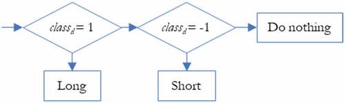
After the ensemble of prediction results, all predicted class_d values are employed in the recommendation of trading one stock as in Figure 3. That is if class_d = 0, then do nothing in response to the uncertainty in direction of price change. If class_d = 1, then take a long position (or buy) of the stock with a proportion ρ of the current available cash. If class_d = – 1, then take a short position (or sell) of the stock for a proportion ρ of the current amount of in-hand stock.

Figure 3. Trading recommendation based on class_d.

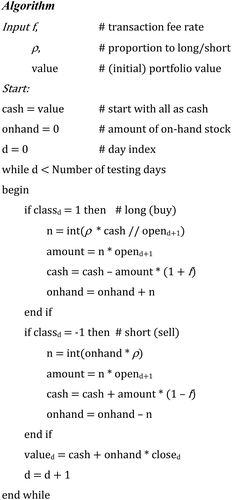
Parameters ρ represents proportion of number of stocks for selling (or short) or amount of cash for buying (long) stocks on the day, thus ρ ∈ (0, 1]. The value of ρ helps control the risk of investment; the lower value of ρ, the more risk averse the investor takes by buying a smaller portion of the current cash and selling a smaller portion of in-hands stocks.

All buying and selling transactions are subjected to transaction fees of rate f. This means that when buying n stocks at price p, we have to pay for n × p × (1 + f). When selling n stocks at price p, our cash will increase only n × p × (1 – f). The trading recommendation and simulation can be summarized as algorithm in Figure 4. The trading decision threshold θ should be greater than the fee rate f to avoid loss from the excessive transaction fee. Note that the proposed algorithm is to be run at the end of day d, and buying or selling transactions as recommended are at the opening price on the next day (open_d+1).

Figure 4. Algorithm for trading recommendation.

Experimentation

Data in the experiment are historical daily prices of 20 stocks from Stock Exchange of Thailand (SET). They are among top largest stocks and are randomly selected from leaders of different major industries including energy, telecommunication, banking, foods, infrastructure, property, etc. To study the performance in varying market situations, the datasets are taken from the following three different periods:

1. 2014-1-2 to 2018–12-28

2. 2015-1-5 to 2019–12-30

3. 2016-1-4 to 2020–12-30

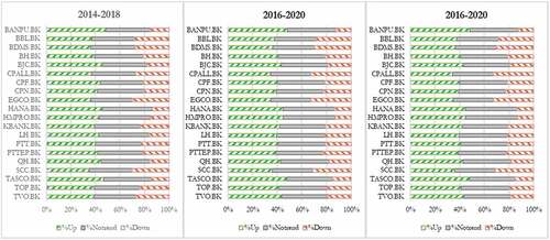
Each dataset ranges 5 years or about 1220 days and is split into 80:20 proportion for training and testing. The training set is for constructing the classification models whose performance will be compared using the testing set. The characteristics of the stocks are summarized in Table 3. Column Sign Diff? indicates that the direction of change in training set is different to the direction of change in testing set. Such different patterns of training set and testing set makes it more difficult to generalize the classification models. Figures 5-7 illustrate charts of the closing prices of all stocks for the three datasets. It can be seen from both Table 3 and the figures that the tested stocks have various characteristics: uptrend, downtrend, fluctuation, and sideway, during the training and testing periods for evaluating the proposed models under varying market situations. Figure 8 illustrates proportion of class_d (or direction of price change) for testing set of each stock. Set {%Up, %Notrend, %Down} maps to {1, 0, −1}. The Figure 8 shows that the classification problem in this work is not imbalance.

Table 3. Characteristics of stocks used in the experiment

Period	2014–2018			2015–2019			2016–2020
Stock	%Chg (Training)	%Chg (Testing)	Sign Diff?	%Chg (Training)	%Chg (Testing)	Sign Diff?	%Chg (Training)	%Chg (Testing)	Sign Diff?
BANPU.BK	−7.8	−28.16		−20.35	−20.13		−1.12	−7.56
BBL.BK	23.49	−0.98	Y	6.84	−21.18	Y	6.33	−25.94	Y
BDMS.BK	92.66	17.54		37.78	6.12		18.18	−20	Y
BH.BK	129.94	−3.35	Y	35.38	−21.39	Y	−29.61	−18.37
BJC.BK	52.07	−21.01	Y	34.97	−15.15	Y	39.9	−17.26	Y
CPALL.BK	96.25	−12.42	Y	61.76	2.85		91.03	−19.38	Y
CPF.BK	−18.69	0.41	Y	−9.72	10.89	Y	56.25	−2.73	Y
CPN.BK	128	−11.8	Y	67.98	−17	Y	38.67	−23.29	Y
EGCO.BK	81.82	14.29		52.15	33.33		117.11	−41.31	Y
HANA.BK	85.15	−27.47	Y	−12.58	7.81	Y	1.45	15.22
HMPRO.BK	110.13	16.92		101.41	5.96		133.33	−14.38	Y
KBANK.BK	62.89	−23.55	Y	−15.91	−18.38		1.69	−25.17	Y
LH.BK	51.43	−5.71	Y	10	−2	Y	7.14	−18.88	Y
PTT.BK	64.23	−2.54	Y	46.03	−4.86	Y	85.92	−3.41	Y
PTTEP.BK	−34.52	7.08	Y	6.07	10.67		123.32	−21.08	Y
QH.BK	48.4	−16.03	Y	−15.09	−4.48		10.43	−9.38	Y
SCC.BK	28.61	−12.1	Y	−3.11	−10.09		−13.33	−3.57
TASCO.BK	364.25	−35.84	Y	123.08	47.22		−47.67	−17.45
TOP.BK	98.15	−37.79	Y	54.97	9.41		11.16	−25.45	Y
TVO.BK	59.46	−10.17	Y	25	2.8		20	22.73
Mean	75.8	−9.6		29.3	0.1		33.5	−13.8

Figure 5. Price charts of all stocks in dataset A (2014–2018). Training and testing datasets are shown in green and blue colors.

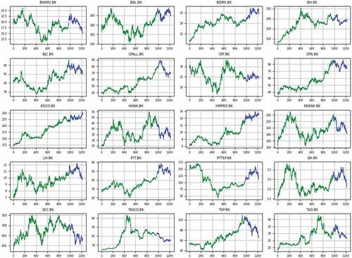
Figure 6. Price charts of all stocks in dataset B (2015–2019). Training and testing datasets are shown in green and blue colors.

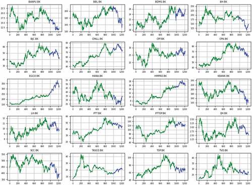
Figure 7. Price charts of all stocks in dataset C (2016–2020). Training and testing datasets are shown in green and blue colors.

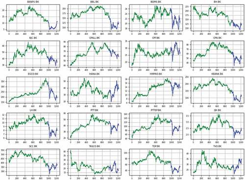
Figure 8. Proportions of % price changes.

Experimentation Setup

Details of the experimentation are as following (see Figure 1):

1. Data Acquisition and Preparation: The downloaded data, including open, high, low, close and volume, are used to calculate 45 technical indicators (whose descriptions are in Table 1) with Python’s TA-Lib library. They forms attributes or features of the dataset. For each dataset range, the downloaded data actually begin at the prior 100 days for necessary calculation of some technical indicators that require historical data; e.g. DISP100 requires data of prior 100 days. Then every feature is normalized to range [0, 1] before further processing.

2. Feature Selection: A filter-based feature selection is employed to pick a subset of 10 optimal features (from the existing 45 attributes) having the highest Chi-square score. We’ve also tried with 8 and 12 features and the results are not significantly different.

3. Training with Hyperparameter Tuning: After feature selection, four base classifiers are trained using the training set. We use Python scikit learn’s gridsearchcv function to exhaustively search for the optimal hyperparameter set of SVM, ANN, RF, XGB, and LGB as reported in subsection 3.4.

4. Prediction and Result Ensemble: After training, five base classifiers are independently used for prediction of daily class_d of the testing set. Their results are then ensembled using algorithm in subsection 3.5 to obtain the prediction results of T3 and E5.

5. Trading Simulation to Observe Performance: The prediction results of all 7 classifiers are further used for simulation using trading recommendation described in subsection 3.5 for comparison. In the simulation, the initial fund is 1,000,000 baht. Note that the amount of initial fund does not matter in this experiment since the performance is based on the investment return R for whole testing period, and R is calculated as following.

(2) $\mathrm{R}=\frac{\mathrm{v}\mathrm{a}\mathrm{l}\mathrm{u}{\mathrm{e}}_{\mathrm{f}}-\mathrm{v}\mathrm{a}\mathrm{l}\mathrm{u}{\mathrm{e}}_{\mathrm{i}}}{\mathrm{v}\mathrm{a}\mathrm{l}\mathrm{u}{\mathrm{e}}_{\mathrm{i}}}$(2)

where value_d = cash_d + onhand_d × close_d, and subscripts i and f denote the initial day and the final day. Term onhand_d denotes the number of stocks held in portfolio on day d. The predicted class_d will be used to make trading decision on day d + 1 as described earlier.

Parameter Setting for Trading Simulation

All buy and sell transactions are subjected to 0.15% commission fee. The decision threshold θ is set to 0.5%. The trading proportion parameter ρ is set to 0.8. These trading parameters are set the same for all trading scenarios for a fair comparison. In fact, we have tested the model with ρ ∈ [0.4, 0.6, 0.8, 1.0]. The results are not significantly different, but the configuration with ρ = 0.8 offers the best results.

Performance Comparison

The above simulation is performed using seven classifiers independently. After the trading simulation, the returns R_SVM, R_ANN, R_RF, R_XGB, R_LGB, R_T3, and R_E5 are to be compared with the returns from the Buy and hold (B&H) strategy, R_BH, as baseline. The return R_BH in this case is computed from the closing price of the last day (close_f) and the opening price of first day (open_i) of the testing dataset, as following:

(3) ${\mathrm{R}}_{\mathrm{B}\mathrm{H}}=\frac{\mathrm{c}\mathrm{l}\mathrm{o}\mathrm{s}{\mathrm{e}}_{\mathrm{f}}-\mathrm{o}\mathrm{p}\mathrm{e}{\mathrm{n}}_{\mathrm{i}}}{\mathrm{o}\mathrm{p}\mathrm{e}{\mathrm{n}}_{\mathrm{i}}}$(3)

The main metrics for comparison are return surplus and Sharpe ratio. Return surplus (Δ) is difference of the return from algorithm and the return from B&H strategy, i.e. ΔT3 = R_T3 – R_BH. A positive surplus means that using the algorithm obtains a higher return than using B&H strategy, and of course the higher Δ achieved, the better the algorithm is.

To measure the volatility or risk of trading, Sharpe ratio (Sr) is the average return earned in excess of the risk-free rate per unit of volatility, represented by the standard deviation σ_p. For good return/risk ratio, Sr should be higher than 1.0. Sr is calculated by

(4) $Sr=\frac{R_p-Rf}{\sigma p}$(4)

where R_p is return rate from investment and Rf or risk-free rate is the return of an investment with risk-free asset, i.e. short-term government treasury bills. In this experiment, Rf is set to 2%, 2% and 0.1% for datasets A, B, and C respectively; these are average values obtained from web Interest Rate of Bank of Thailand (https://www.bot.or.th/English/Statistics/FinancialMarkets/InterestRate/Pages/InterestRate.aspx).

It’s also interesting to observe the case of If we know the future (KF). The return R_KF is computed based on the formulae which is similar to the case of prediction. However, the trading decision (buying, selling or do-nothing) is based on the actual class values, as if we know the future closing prices.

(5) $R_{KF}=\frac{\mathrm{v}\mathrm{a}\mathrm{l}\mathrm{u}{\mathrm{e}}_{\mathrm{f}}-\mathrm{v}\mathrm{a}\mathrm{l}\mathrm{u}{\mathrm{e}}_{\mathrm{i}}}{\mathrm{v}\mathrm{a}\mathrm{l}\mathrm{u}{\mathrm{e}}_{\mathrm{i}}}$(5)

Obviously, if we know the future, the return from trading (R_KF) is very high. This is confirmed from the column R_KF in Table 4. It unquestionably beats other trading strategies for every stock and thus is regarded as the ideal case. Therefore, we here will focus on only the cases of seven classifiers compared with B&H strategy.

Table 4. Results of accuracy values and returns of trading

Dataset A. 2014 – 2018
Name	RBH	RKF	ACSVM	RSVM	ACANN	RANN	ACRF	RRF	ACXGB	RXGB	ACLGB	RLGB	RT3	RE5
BANPU.BK	-25.243	153.675	0.475	0	0.475	0.323	0.475	-2.063	0.484	7	0.516	6.335	3.416	0.863
BBL.BK	-2.913	68.532	0.328	0	0.287	-7.698	0.377	17.738	0.365	9.112	0.377	15.635	9.242	12.011
BDMS.BK	15.094	144.179	0.348	13.828	0.365	11.121	0.283	8.786	0.275	1.69	0.398	25.249	14.112	-0.433
BH.BK	-5.641	123.939	0.439	7.238	0.455	8.014	0.447	1.434	0.434	-1.638	0.381	-12.734	2.531	-0.005
BJC.BK	-21.875	131.069	0.381	-2.557	0.393	0	0.393	-5.524	0.357	1.924	0.439	32.505	2.507	5.326
CPALL.BK	-12.975	84.184	0.287	-12.493	0.324	-5.834	0.393	9.594	0.398	2.365	0.348	-13.307	-0.266	-1.886
CPF.BK	-2.033	106.462	0.398	2.483	0.410	6.069	0.414	13.076	0.422	2.045	0.402	1.677	4.189	6.893
CPN.BK	-13.864	82.193	0.447	-0.167	0.439	-0.413	0.467	-0.517	0.439	1.931	0.455	-5.671	3.558	-1.163
EGCO.BK	12.442	88.371	0.385	13.675	0.377	2.756	0.389	14.901	0.410	22.879	0.422	20.428	21.538	18.361
HANA.BK	-30.22	182.606	0.512	1.202	0.475	6.139	0.439	-21.663	0.434	-19.594	0.459	-17.842	-21.449	-10.487
HMPRO.BK	13.74	142.904	0.463	19.598	0.516	34.704	0.459	10.595	0.467	17.22	0.475	11.8	23.154	13.372
KBANK.BK	-24.38	99.788	0.406	-6.792	0.418	-11.625	0.463	-1.798	0.393	-8.934	0.406	-19.155	-2.134	1.081
LH.BK	-8.019	95.108	0.389	6.753	0.406	4.69	0.418	9.032	0.439	13.921	0.422	12.282	4.879	5.19
PTT.BK	-3.072	153.270	0.393	-4.844	0.434	1.9	0.459	6.521	0.393	-12.408	0.422	-4.919	-9.212	-6.498
PTTEP.BK	6.542	221.384	0.357	0	0.393	15.519	0.381	16.703	0.377	6.519	0.393	22.284	23.336	36.434
QH.BK	-16.561	129.308	0.484	0	0.492	2.589	0.488	5.521	0.496	8.917	0.443	-2.566	5.869	6.742
SCC.BK	-12.903	67.318	0.381	7.195	0.336	-3.226	0.430	-4.263	0.357	-8.294	0.365	-12.415	-8.008	-1.692
TASCO.BK	-35.841	207.807	0.529	0	0.443	-18.351	0.484	-16.31	0.459	-2.293	0.447	-25.289	-19.414	-22.539
TOP.BK	-38.152	142.087	0.410	-22.21	0.357	-35.495	0.414	-20.129	0.426	-24.097	0.398	-34.913	-25.589	-23.008
TVO.BK	-10.924	138.971	0.439	2.562	0.475	2.145	0.459	-4.024	0.480	6.424	0.422	-9.373	-1.553	2.195

Dataset B. 2015 – 2019
Name	RBH	RKF	ACSVM	RSVM	ACANN	RANN	ACRF	RRF	ACXGB	RXGB	ACLGB	RLGB	RT3	RE5
BANPU.BK	-20.667	160.750	0.537	0	0.545	12.681	0.516	13.013	0.516	16.988	0.549	18.698	14.815	28.473
BBL.BK	-21.814	65.005	0.402	0	0.430	-9.102	0.393	-6.88	0.385	-9.833	0.381	-7.66	-3.873	-9.105
BDMS.BK	6.122	111.213	0.340	7.515	0.332	1.554	0.434	22.529	0.377	3.023	0.320	-4.498	9.416	5.43
BH.BK	-22.281	102.538	0.385	-10.257	0.402	-8.335	0.398	-16.958	0.410	3.658	0.369	-21.352	-16.311	-6.381
BJC.BK	-13.065	120.869	0.426	0	0.418	-5.751	0.467	5.98	0.451	-1.276	0.467	9.684	16.116	6.797
CPALL.BK	4.965	84.797	0.332	4.597	0.348	6.551	0.377	-3.706	0.348	2.742	0.393	5.307	2.538	3.411
CPF.BK	10	140.335	0.353	3.15	0.348	0	0.426	25.88	0.418	28.6	0.443	24.707	30.647	26.371
CPN.BK	-16.333	95.276	0.393	-8.162	0.393	-3.826	0.398	-0.451	0.398	-2.23	0.414	-3.963	2.797	4.822
EGCO.BK	34.146	143.653	0.312	-2.331	0.287	4.678	0.328	-6.366	0.385	4.295	0.361	9.745	17.463	-5.762
HANA.BK	10.236	276.257	0.406	-8.707	0.402	-0.133	0.443	-2.475	0.459	16.206	0.492	30.645	11.766	3.667
HMPRO.BK	7.285	103.741	0.451	8.531	0.488	24.299	0.508	9.656	0.434	4.445	0.455	16.051	14.13	21.002
KBANK.BK	-19.571	105.524	0.426	-1.317	0.410	-4.843	0.422	7.716	0.443	7.361	0.410	-8.997	14.03	9.114
LH.BK	-2	74.199	0.377	4.871	0.361	-1.017	0.381	-1.234	0.406	-2.764	0.426	6.46	0.328	0.881
PTT.BK	-4.839	84.675	0.496	0	0.500	1.97	0.336	-8.191	0.320	-9.233	0.398	-7.332	-7.1	-3.322
PTTEP.BK	10.573	119.194	0.361	0	0.316	2.535	0.353	6.298	0.344	-4.037	0.373	14.512	11.273	-0.555
QH.BK	-5.224	79.658	0.414	0	0.410	1.241	0.434	0.82	0.406	3.766	0.459	6.496	7.719	9.169
SCC.BK	-10.502	75.854	0.385	-2.981	0.385	-1.989	0.381	-7.199	0.385	-11.208	0.353	-5.259	-5.059	-3.343
TASCO.BK	41.781	250.891	0.406	0	0.402	-3.573	0.406	13.475	0.422	29.601	0.406	8.582	22.683	11.077
TOP.BK	8.108	186.200	0.389	14.838	0.389	0	0.422	27.096	0.426	32.565	0.414	35.591	43.655	39.199
TVO.BK	3.774	99.555	0.430	0	0.439	0.189	0.443	14.187	0.430	3.762	0.459	11.829	13.779	12.382

Dataset C. 2016 – 2020
Name	RBH	RKF	ACSVM	RSVM	ACANN	RANN	ACRF	RRF	ACXGB	RXGB	ACLGB	RLGB	RT3	RE5
BANPU.BK	-5	897.537	0.459	0	0.459	0	0.5164	20.17	0.373	-48.498	0.4959	-0.042	6.878	-35.798
BBL.BK	-24.224	336.123	0.3484	-24.304	0.3484	-20.503	0.3852	-17.94	0.3852	-18.983	0.4344	-2.644	0.793	-12.355
BDMS.BK	-18.846	176.694	0.3811	-15.001	0.3402	-11.027	0.3975	-17.345	0.3893	-4.296	0.3074	-25.983	-8.64	-13.212
BH.BK	-16.949	371.764	0.4508	0	0.4836	-10.2	0.4549	-8.134	0.4918	16.354	0.4795	-10.29	8.86	8.532
BJC.BK	-16.667	409.589	0.5	37.432	0.5082	3.119	0.4672	24.954	0.4754	8.27	0.4344	0.247	11.622	36.211
CPALL.BK	-18.276	158.64	0.3484	-9.832	0.3525	-18.501	0.3893	-0.839	0.4344	26.724	0.3648	20.516	16.259	9.416
CPF.BK	-0.909	296.664	0.4672	6.203	0.4672	10.811	0.4549	2.746	0.4713	11.206	0.5123	22.095	11.907	19.921
CPN.BK	-20.884	544.397	0.4549	-4.868	0.4836	-0.218	0.4713	-9.265	0.4303	-23.472	0.4344	-16.204	-8.69	-9.362
EGCO.BK	-40.455	277.202	0.2787	-37.933	0.2336	-40.384	0.3238	-38.556	0.3484	-29.074	0.3156	-11.422	-24.326	-36.461
HANA.BK	13.768	904.633	0.4795	-11.844	0.5328	20.369	0.4836	23.722	0.4836	16.209	0.4795	18.332	17.041	9.064
HMPRO.BK	-14.286	399.591	0.4631	6.89	0.459	-4.008	0.5	-6.596	0.5082	5.609	0.4918	-4.67	6.412	-4.775
KBANK.BK	-23.432	541.116	0.5041	0	0.377	-42.943	0.4139	-9.229	0.418	3.316	0.4098	-12.502	-9.956	-9.143
LH.BK	-17.347	251.482	0.3893	-9.377	0.4713	16.814	0.4385	-14.606	0.4221	-3.477	0.4262	-13.174	-13.923	13.474
PTT.BK	-2.26	409.392	0.4467	0	0.5164	2.383	0.4754	-2.134	0.4016	12.254	0.459	10.25	-1.321	-8.973
PTTEP.BK	-21.713	614.184	0.3975	-22.329	0.3852	-31.364	0.4754	-0.567	0.4057	-4.822	0.4877	-4.157	-1.348	-13.318
QH.BK	-9.375	172.429	0.418	-10.885	0.4385	15.667	0.4057	-4.85	0.4098	-8.451	0.4713	34.06	-0.92	11.112
SCC.BK	-2.296	198.313	0.3934	22.081	0.2705	-14.064	0.4139	9.933	0.4754	37.335	0.4385	20.546	33.902	28.057
TASCO.BK	-16.038	521.015	0.4426	0	0.4426	0	0.4426	15.466	0.4672	22.448	0.459	13.026	23.323	3.181
TOP.BK	-23.929	989.786	0.4795	-18.512	0.5861	36.088	0.4713	-9.644	0.5164	-13.581	0.4795	-25.987	-16.396	23.854
TVO.BK	27.523	323.796	0.4426	0	0.4385	3.68	0.4836	58.248	0.4836	25.628	0.4713	50.331	59.926	38.302

In addition, we investigate the relationship of return of proposed ensemble model and accuracy metric. Accuracy (Ac) is the total number of correct predictions divided by the total number of predictions made for a dataset.

Results and Discussions

Table 4 lists accuracies of predictions and returns of trading from seven classifiers using the same testing dataset (A, B, and C separately). For a better comparison, Table 5 reports the return surpluses (Δ) of all 7 classifiers. Then their averages, together with average Sharpe ratios (Sr) and average accuracies (Ac), are displayed in Table 6. The higher Δ indicates more profit given by such algorithm, whereas the higher Sr reflects a better excess return per risk. As a baseline reference, Table 7 reports the averages of returns from B&H (R_BH). To identify the superior performance among 7 classifiers, their returns are ranked from 1 (best) to 7 (worst) for 20 stocks. Next, those 20 ranks are averaged for each classifier and listed in Table 8 as average rank. Table 9 reports the correlation coefficients (Cor) of return and accuracy of all classifiers. Figure 9 illustrates the comparative returns of all classifiers over testing periods for some largest stocks in different sectors.

Figure 9. Comparative returns for some largest stocks.

Figure 9. Continued.

Table 5. Return Surpluses ΔX = R_X – R_BH

Dataset A. 2014 – 2018
Stock	ΔSVM	ΔANN	ΔRF	ΔXGB	ΔLGB	ΔT3	ΔE5
BANPU.BK	25.24	25.57	23.18	32.24	31.58	28.66	26.11
BBL.BK	2.91	-4.79	20.65	12.03	18.55	12.16	14.92
BDMS.BK	-1.27	-3.97	-6.31	-13.40	10.16	-0.98	-15.53
BH.BK	12.88	13.66	7.08	4.00	-7.09	8.17	5.64
BJC.BK	19.32	21.88	16.35	23.80	54.38	24.38	27.20
CPALL.BK	0.48	7.14	22.57	15.34	-0.33	12.71	11.09
CPF.BK	4.52	8.10	15.11	4.08	3.71	6.22	8.93
CPN.BK	13.70	13.45	13.35	15.80	8.19	17.42	12.70
EGCO.BK	1.23	-9.69	2.46	10.44	7.99	9.10	5.92
HANA.BK	31.42	36.36	8.56	10.63	12.38	8.77	19.73
HMPRO.BK	5.86	20.96	-3.14	3.48	-1.94	9.41	-0.37
KBANK.BK	17.59	12.75	22.58	15.45	5.22	22.25	25.46
LH.BK	14.77	12.71	17.05	21.94	20.30	12.90	13.21
PTT.BK	-1.77	4.97	9.59	-9.34	-1.85	-6.14	-3.43
PTTEP.BK	-6.54	8.98	10.16	-0.02	15.74	16.79	29.89
QH.BK	16.56	19.15	22.08	25.48	14.00	22.43	23.30
SCC.BK	20.10	9.68	8.64	4.61	0.49	4.90	11.21
TASCO.BK	35.84	17.49	19.53	33.55	10.55	16.43	13.30
TOP.BK	15.94	2.66	18.02	14.06	3.24	12.56	15.14
TVO.BK	13.49	13.07	6.90	17.35	1.55	9.37	13.12

Dataset B. 2015 – 2019
Stock	ΔSVM	ΔANN	ΔRF	ΔXGB	ΔLGB	ΔT3	ΔE5
BANPU.BK	20.67	33.35	33.68	37.66	39.37	35.48	49.14
BBL.BK	21.81	12.71	14.93	11.98	14.15	17.94	12.71
BDMS.BK	1.39	-4.57	16.41	-3.10	-10.62	3.29	-0.69
BH.BK	12.02	13.95	5.32	25.94	0.93	5.97	15.90
BJC.BK	13.07	7.31	19.04	11.79	22.75	29.18	19.86
CPALL.BK	-0.37	1.59	-8.67	-2.22	0.34	-2.43	-1.55
CPF.BK	-6.85	-10.00	15.88	18.60	14.71	20.65	16.37
CPN.BK	8.17	12.51	15.88	14.10	12.37	19.13	21.15
EGCO.BK	-36.48	-29.47	-40.51	-29.85	-24.40	-16.68	-39.91
HANA.BK	-18.94	-10.37	-12.71	5.97	20.41	1.53	-6.57
HMPRO.BK	1.25	17.01	2.37	-2.84	8.77	6.85	13.72
KBANK.BK	18.25	14.73	27.29	26.93	10.57	33.60	28.69
LH.BK	6.87	0.98	0.77	-0.76	8.46	2.33	2.88
PTT.BK	4.84	6.81	-3.35	-4.39	-2.49	-2.26	1.52
PTTEP.BK	-10.57	-8.04	-4.28	-14.61	3.94	0.70	-11.13
QH.BK	5.22	6.47	6.04	8.99	11.72	12.94	14.39
SCC.BK	7.52	8.51	3.30	-0.71	5.24	5.44	7.16
TASCO.BK	-41.78	-45.35	-28.31	-12.18	-33.20	-19.10	-30.70
TOP.BK	6.73	-8.11	18.99	24.46	27.48	35.55	31.09
TVO.BK	-3.77	-3.59	10.41	-0.01	8.06	10.00	8.61

Dataset C. 2016 – 2020
Stock	ΔSVM	ΔANN	ΔRF	ΔXGB	ΔLGB	ΔT3	ΔE5
BANPU.BK	5.00	5.00	25.17	-43.50	4.96	11.88	-30.80
BBL.BK	-0.08	3.72	6.28	5.24	21.58	25.02	11.87
BDMS.BK	3.84	7.82	1.50	14.55	-7.14	10.21	5.63
BH.BK	16.95	6.75	8.82	33.30	6.66	25.81	25.48
BJC.BK	54.10	19.79	41.62	24.94	16.91	28.29	52.88
CPALL.BK	8.44	-0.23	17.44	45.00	38.79	34.54	27.69
CPF.BK	7.11	11.72	3.66	12.12	23.00	12.82	20.83
CPN.BK	16.02	20.67	11.62	-2.59	4.68	12.19	11.52
EGCO.BK	2.52	0.07	1.90	11.38	29.03	16.13	3.99
HANA.BK	-25.61	6.60	9.95	2.44	4.56	3.27	-4.70
HMPRO.BK	21.18	10.28	7.69	19.90	9.62	20.70	9.51
KBANK.BK	23.43	-19.51	14.20	26.75	10.93	13.48	14.29
LH.BK	7.97	34.16	2.74	13.87	4.17	3.42	30.82
PTT.BK	2.26	4.64	0.13	14.51	12.51	0.94	-6.71
PTTEP.BK	-0.62	-9.65	21.15	16.89	17.56	20.37	8.40
QH.BK	-1.51	25.04	4.52	0.92	43.44	8.46	20.49
SCC.BK	24.38	-11.77	12.23	39.63	22.84	36.20	30.35
TASCO.BK	16.04	16.04	31.50	38.49	29.06	39.36	19.22
TOP.BK	5.42	60.02	14.28	10.35	-2.06	7.53	47.78
TVO.BK	-27.52	-23.84	30.72	-1.89	22.81	32.40	10.78

Table 6. Averages of return surplus (ΔX = R_X – R_BH), Sharpe ratios (Sr), and accuracy (Ac)

Metric	Dataset	SVM	ANN	RF	XGB	LGB	T3	E5
Average Δ	A. 2014 – 2018	12.113	11.506	12.720	12.074	10.340	12.375	12.878
	B. 2015 – 2019	0.453	0.822	4.625	5.787	6.928	10.006	7.632
	C. 2016 – 2020	7.966	8.366	13.356	14.115	15.696	18.150	15.466
$\bar{\mathrm{\Delta }}$	Grand average	6.844	6.898	10.234	10.659	10.988	13.510	11.992
Average Sr	A. 2014 – 2018	0.394	0.040	0.476	0.265	-0.298	0.755	0.916
	B. 2015 – 2019	-0.063	-0.587	0.710	1.134	1.006	1.261	1.160
	C. 2016 – 2020	-0.063	-0.009	0.710	0.910	1.071	1.586	1.225
$\overline{Sr}$	Grand average	0.089	-0.185	0.632	0.770	0.593	1.201	1.100
Average Ac	A. 2014 – 2018	0.412	0.414	0.427	0.415	0.419	0.423	0.445
	B. 2015 – 2019	0.401	0.400	0.413	0.408	0.417	0.497	0.463
	C. 2016 – 2020	0.427	0.430	0.443	0.440	0.443	0.481	0.476
$\overline{Ac}$	Grand average	0.414	0.414	0.428	0.421	0.426	0.467	0.461

Table 7. Averages of returns from B&H (R_BH)

Dataset	Average RBH
A. 2014–2018	−10.840
B. 2015–2019	.035
C. 2016–2020	−12.580
Grand average RBH	−7.795

Table 8. Average ranks of return

Dataset	SVM	ANN	RF	XGB	LGB	T3	E5
A. 2014–2018	3.90	4.30	3.90	3.75	4.85	3.65	3.65
B. 2015–2019	4.80	4.55	4.50	4.60	3.75	2.65	3.15
C. 2016–2020	4.65	4.50	4.30	3.45	4.10	2.95	3.95
Average	4.45	4.45	4.23	3.93	4.23	3.08	3.58

Table 9. Correlation coefficients (Cor) of return and accuracy

Dataset	SVM	ANN	RF	XGB	LGB	T3	E5
A. 2014–2018	0.142	0.433	−0.388	0.157	0.115	0.327	0.284
B. 2015–2019	−0.065	0.300	0.489	0.517	0.555	0.479	0.463
C. 2016–2020	0.607	0.000	0.788	0.000	0.599	0.541	0.516
Average Cor	0.228	0.244	0.296	0.225	0.423	0.449	0.421

Here are the observations from Tables 6 to 9.

(1) In Table 6, all average Δs are greater than 0, indicating that on average the proposed trading recommendation provides a more profitable return than B&H.

(2) Among three datasets: A, B & C, T3 outperforms all base classifiers, except in dataset A (ΔT3 = 12.375 < ΔRF = 12.720). In addition, E5 outperforms all base classifiers, except in dataset C (ΔE5 = 15.466 < ΔLGB = 15.696).

(3) T3 and E5 defeat all individual base classifiers in terms of the average $\bar{\mathrm{\Delta }}$ of three datasets: $\bar{\mathrm{\Delta }}$ _T3 = 13.513 (the highest), $\bar{\mathrm{\Delta }}$ _E5 = 11.993 (the second best), with ranking as $\bar{\mathrm{\Delta }}$ _T3 > $\bar{\mathrm{\Delta }}$ _E5 > $\bar{\mathrm{\Delta }}$ _LGB > $\bar{\mathrm{\Delta }}$ _XGB > $\bar{\mathrm{\Delta }}$ _RF > $\bar{\mathrm{\Delta }}$ _ANN > $\bar{\mathrm{\Delta }}$ _SVM.

(4) Majority of average Sr are below 1.0, corresponding to the fluctuated downtrend or sideway of price charts in Figure 5–7 and confirmed by the averages of R_BH in Table 7. Considering those Sr > 1.0 (bold font), both T3 and E5 can achieve the highest $\overline{Sr}$ on average.

(5) In Table 8, T3 achieves the best average rank (lowest value) in all three datasets.

(6) Based on above discussions, modern ensemble-based classifiers (XGB and LGB) outperform classical SVM, ANN, and RF. And more importantly, the proposed T3 and E5 outperform all base classifiers on average in terms of both return and Sharpe ratio.

The following are discussions on accuracies and returns.

(7) In Table 6, T3 and E5 defeat all individual base classifiers in terms of average accuracies of 3 datasets: $\overline{Ac}$ _T3 = 0.467 (the highest), $\overline{Ac}$ _E5 = 0.461 (the second), with ranking as $\overline{Ac}$ _T3 > $\overline{Ac}$ _E5 > $\overline{Ac}$ _RF > $\overline{Ac}$ _LGB > $\overline{Ac}$ _XGB > $\overline{Ac}$ _SVM = $\overline{Ac}$ _ANN.

(8) In Table 9, LGB, T3 and E5 have average values of Cor greater than 0.40, which are higher than other classifiers. A higher positive value of Cor signifies a stronger relationship between return and accuracy achieved by the classifier. T3 achieves the highest Cor value in this case, and LGB ranked second. Considering this together with $\overline{Ac}$ (in Table 7) and average rank of return (in Table 8), we can observe that the selective majority voting scheme of T3 clearly helps improve the accuracy and return.

(9) In summary, the proposed T3 with majority voting of the 3 (out of 5) classifiers with the highest accuracy outperforms the E5 with straightforward majority voting as well as other base classifiers.

Conclusion and Future Works

This work brings together five widely used classifiers for trend prediction. The proposed ensemble classifier T3 combines the results from base classifiers with a selective majority voting by dropping out the results from two classifiers with lowest accuracies. Hyperparameters of each base classifier are tuned with an exhaustive grid search method. The prediction results are further used for recommendation (to buy, to sell, or to do nothing) in a single-stock trading simulation. Performance of all classifiers are compared using historical daily prices of 20 leading stocks in Stock Exchange of Thailand (SET). The inputs of classifiers are 45 technical indicators calculated and taken through a feature selection process. Empirical results reveal that the proposed ensemble T3 model clearly achieves a higher trading return and Sharpe ratio than B&H strategy, all individual base classifiers, and the ensemble with straightforward majority voting (E5). In addition, novel ensemble-based classifiers like XGBoost and LightGBM have better performance than more classical classifiers in this experiment.

Limitations and future works: However major limitations of this work are (i) do not support short-selling which is in a roadmap of full adoption world-wide and in SET, (ii) do not incorporate stop-loss mechanism, (iii) trading recommendation is limited to a single stock. Future works shall support short-selling, multistock trading recommendation with stop-loss mechanism and using other classifiers with profitability-concerned metrics, more advanced ensemble methods, feature selection methods. Other data sources including fundamentals and online news should also be considered.

Disclosure statement

No potential conflict of interest was reported by the author(s).

References

- Ampomah, E. K., Z. Qin, and G. Nyame. 2020. Evaluation of tree-based ensemble machine learning models in predicting stock price direction of movement. Information 11 (6):226. doi:10.3390/info11060332.
- Bose, N. K., and P. Liang. 1996. Neural network fundamentals with graphs, algorithms, and applications. In McGraw-Hill series in electrical and computer engineering, ed. S. W. Director. 1-30. New York: McGraw-Hill.
- Breiman, L. 1996. Bagging predictors. Machine Learning 24:123–257. doi:10.1007/BF00058655.
- Breiman, L. 2001. Random forests. Machine Learning 45 (1):5–32. doi:10.1023/A:1010933404324.
- Cai, J., J. Luo, S. Wang, and S. Yang. 2018. Feature selection in machine learning: A new perspective. Neurocomputing 300:70–79. doi:10.1016/j.neucom.2017.11.077.
- Chen, A.-S., M.-T. Leung, and H. Daouk. 2003. Application of neural networks to an emerging financial market: Forecasting and trading the Taiwan Stock Index. Computer and Operation Research 30 (6):901–23. doi:10.1016/S0305-0548(02)00037-0.
- Chen, T., and C. Guestrin. 2016. XGBoost: A Scalable Tree Boosting System. Proceedings of the 22nd ACM SIGKDD international conference on knowledge discovery and data mining August 13 - 17, 2016 San Francisco, California, 785–94. doi:10.1145/2939672.2939785.
- Chen, W., H. Zhang, M. K. Mehlawat, and L. Jia. 2021. Mean–variance portfolio optimization using machine learning-based stock price prediction. Applied Soft Computing 100:106943. doi:10.1016/j.asoc.2020.106943.
- Cortes, C., and V. Vapnik. 1995. Support-vector networks. Machine Learning 20 (3):273–97. doi:10.1007/BF00994018.
- Deng, S., X. Huang, Z. Qin, Z. Fu, and T. Yang. 2021. A novel hybrid method for direction forecasting and trading of Apple Futures. Applied Soft Computing 110:107734. doi:10.1016/j.asoc.2021.107734.
- Ding, G., and L. Qin. 2020. Study on the prediction of stock price based on the associated network model of LSTM. International Journal of Machine Learning and Cybernetics 11:1307–17. doi:10.1007/s13042-019-01041-1.
- Elshawi, R., M. Maher, and S. Sakr. 2019. Automated machine learning: State-of-the-art and open challenges. arXiv Preprint arXiv:1906.02287, 1–26. http://arxiv.org/abs/1906.02287 .
- Friedman, J. H. 2001. Greedy function approximation: A gradient boosting machine. The Annals of Statistics 29 (5):1189–232. doi:10.1214/aos/1013203451.
- Guang, L., and X. Wang. 2019. A new metric for individual stock trend prediction. Engineering Applications of Artificial Intelligence 82:1–12. doi:10.1016/j.engappai.2019.03.019.
- Hu, Y., K. Liu, X. Zhang, L. Su, E.-W.-T. Ngai, and M. Liu. 2015. Application of evolutionary computation for rule discovery in stock algorithmic trading: A literature review. Applied Soft Computing 36:534–51. doi:10.1016/j.asoc.2015.07.008.
- Huang, W., Y. Nakamori, and S.-Y. Wang. 2005. Forecasting stock market movement direction with support vector machine. Computers & Operations Research 32:2513–22. doi:10.1016/j.cor.2004.03.016.
- Hussain, A. J., A. Knowles, P. J. G. Lisboa, and W. El-Deredy. 2008. Financial time series prediction using polynomial pipelined neural networks. Expert Systems and Applications 35 (3):1186–99. doi:10.1016/j.eswa.2007.08.038.
- Kara, Y., M. A. Boyacioglu, and Ö. K. Baykan. 2011. Predicting direction of stock price index movement using artificial neural networks and support vector machines: The sample of the Istanbul stock exchange. Expert Systems with Applications 38 (5):5311–19. doi:10.1016/j.eswa.2010.10.027.
- Ke, G. et al, 2017. Lightgbm: A highly efficient gradient boosting decision tree. Advances in Neural Information Processing Systems 30:3149–54.
- Khairalla, M. A., X. Ning, N. T. AL-Jallad, and M. O. El-Faroug. 2018. Short-term forecasting for energy consumption through stacking heterogeneous ensemble learning model. Energies 2018 (11):1–21. doi:10.3390/en11061605.
- Kim, H., and S.-T. Han. 2016. The enhanced classification for the stock index prediction. Procedia Computer Science 91:284–86. doi:10.1016/j.procs.2016.07.077.
- Li, J., K. Cheng, S. Wang, F. Morstatter, R. P. Trevino, J. Tang, and H. Liu. 2018. Feature Selection: A data perspective. ACM Computing Survey (CSUR) 50 (6):94. doi:10.1145/3136625.
- Lorenzo, R. D. 2013. Basic Technical analysis of financial markets: A modern approach. Heidelberg: Springer Milan.
- Luo, L., S. You, Y. Xu, and H. Peng. 2017. Improving the integration of piece wise linear representation and weighted support vector machine for stock trading signal prediction. Applied Soft Computing 56:199–216. doi:10.1016/j.asoc.2017.03.007.
- Nguyen, B. H., B. Xue, and M. Zhang. 2020. A survey on swarm intelligence approaches to feature selection in data mining. Swarm and Evolutionary Computation 54:100633–49. doi:10.1016/j.swevo.2020.100663.
- Ni, L. P., Z. W. Ni, and Y. Z. Gao. 2011. Stock trend prediction based on fractal feature selection and support vector machine. Expert Systems with Applications 38 (5):5569–76. doi:10.1016/j.eswa.2010.10.079.
- Nobre, J., and R. Neves. 2019. Combining principal component analysis, discrete wavelet transform and XGBoost to trade in the financial markets. Expert Systems with Applications 125:181–94. doi:10.1016/j.eswa.2019.01.083.
- Nti, I. K., A. F. Adekoya, and B. A. Weyori. 2020a. A comprehensive evaluation of ensemble learning for stock-market prediction. Journal of Big Data 7 (20). doi:10.1186/s40537-020-00299-5.
- Nti, I. K., A. F. Adekoya, and B. A. Weyori. 2020b. Efficient stock-market prediction using ensemble support vector machine. Open Computer Science 10 (1):153–63. doi:10.1515/comp-2020-0199.
- O’Connor, N., and M. G. Madden. 2006. A neural network approach to predicting stock exchange movements using external factors. Knowledge Based Systems 19 (5):371–78. doi:10.1016/j.knosys.2005.11.015.
- Olson, D., and C. Mossman. 2003. Neural network forecasts of Canadian stock returns using accounting ratios. International Journal of Forecasting 19 (3):453–65. doi:10.1016/S0169-2070(02)00058-4.
- Oram, E., P.-B. Dash, B. Naik, J. Nayak, S. Vimal, and S. K. Nataraj. 2021. Light gradient boosting machine-based phishing webpage detection model using phisher website features of mimic URLs. Pattern Recognition Letters 152:100–06. doi:10.1016/j.patrec.2021.09.018.
- Polikar, R. 2006. Ensemble based systems in decision making. IEEE Circuits and Systems Magazine 6:21–45. doi:10.1109/MCAS.2006.1688199.
- Sharpe, W. F. 1994. The Sharpe Ratio. The Journal of Portfolio Management 21 (1):49–58. doi:10.3905/jpm.1994.409501.
- Slezak, J., L. Butler, and O. Akbilgic. 2021. The role of frailty index in predicting readmission risk following total joint replacement using light gradient boosting machines. Informatics in Medicine Unlocked 25:100657–62. doi:10.1016/j.imu.2021.100657.
- Teixeira, L. A., and A. L. I. De Oliveira. 2010. A method for automatic stock trading combining technical analysis and nearest neighbor classification. Expert Systems with Applications 37 (10):6885–90. doi:10.1016/j.eswa.2010.03.033.
- Thakur, M., and D. Kumar. 2018. A hybrid financial trading support system using multi-category classifiers and random forest. Applied Soft Computing 67:337–49. doi:10.1016/j.asoc.2018.03.006.
- Tsai, C.-F., Y.-C. Lin, D.-C. Yen, and Y.-M. Chen. 2011. Predicting stock returns by classifier ensembles. Applied Soft Computing 11 (2):2452–59. doi:10.1016/j.asoc.2010.10.001.
- Wang, J.-Z., -J.-J. Wang, Z.-G. Zhang, and S.-P. Guo. 2011. Forecasting stock indices with back propagation neural network. Expert Systems with Applications 38 (11):14346–55. doi:10.1016/j.eswa.2011.04.222.
- Wolpert, D.-H., and W.-G. Macready. 1997. No free lunch theorems for search. IEEE Transactions on Evolutionary Computation 1:67–82. doi:10.1109/4235.585893.
- Xue, B., M. Zhang, W. Browne, and X. Yao. 2016. A survey on evolutionary computation approaches to feature selection. IEEE Transactions on Evolutionary Computation 20:606–26. doi:10.1109/TEVC.2015.2504420.
- Yang, L., and A. Shami. 2020. On hyperparameter optimization of machine learning algorithms: Theory and practice. Neurocomputing 415:295–316. doi:10.1016/j.neucom.2020.07.061.
- Yun, K. K., S. W. Yoon, and D. Won. 2021. Prediction of stock price direction using a hybrid GA-XGBoost algorithm with a three-stage feature engineering process. Expert Systems with Applications 186:115716. doi:10.1016/j.eswa.2021.115716.
- Zhang, J., S. Cui, Y. Xu, Q. Li, and T. Li. 2018. A novel data-driven stock price trend prediction system. Expert Systems with Applications 97:60–69. doi:10.1016/j.eswa.2017.12.026.
- Zhang, Y., W. Yu, Z. Li, S. Raza, and H. Cao. 2021. Detecting ethereum Ponzi schemes based on improved LightGBM algorithm. IEEE Transactions on Computational Social Systems. doi:10.1109/TCSS.2021.3088145.