Understanding Bias and Variance of Learning-to-Rank Algorithms: An Empirical Framework

ABSTRACT

Learning-to-rank (LtR) algorithms are at the heart of modern day information retrieval systems. While a good number of LtR algorithms have been developed and scrutinized over the past decade, theoretical underpinnings of these algorithms are not thoroughly investigated so far. Amongst the theoretical aspects of a supervised learning algorithm, the bias-variance profiles are of utmost importance. In this article we aim to better understand the bias-variance profiles of rank-learning algorithms. Firstly, we formalize the bias and variance from a pointwise perspective where each query-document pair is treated as an individual training example. Secondly, we develop a framework to analyze the variability and systematic error of a rank-learner in terms of its ranking error, i.e., we analyze the bias-variance from a listwise perspective where a query and all of its associated documents are treated as a single training example. After developing the theoretical framework, we move on to test its applicability in practice. In particular, we choose a promising algorithm, namely random forest-based rank-learning algorithms for our investigation. We study the effect of varying an important parameter of the algorithm, namely the sub-sample size used to learn each tree, on bias and variance. Our hypothesis is that as the sub-sample size (per tree) increases, classical bias-variance tradeoff should be observed. On two large LtR benchmark datasets, experimental results show that our hypothesis holds true. We also explain the relative performance of two of the top performing LtR algorithms using their bias and variance profiles. To the best of our knowledge, this article presents the first thorough investigation into bias and variance analysis of rank-learning algorithms.

1. Introduction

Supervised machine learning algorithms learn a function, specifically, the parameters of a function, from labeled training data where the training data consist of different signals about the labels of training examples. The learnt function is then used to predict the labels of unseen examples. In a learning-to-rank (LtR) scenario, a training example consists of the scores of various classical retrieval functions (such as cosine similarity score, BM25 score etc. (Manning, Raghavan, and Schütze 2008)) for a query-document pair, and the true relevance label for the document in question is considered to be the ground truth label. A scoring function is then learnt during training. This function, during evaluation, takes an unseen example, i.e., a query-document pair as argument and predicts a relevance score for that example. All the documents are then sorted in decreasing order of these predicted scores and presented to the user of the information retrieval (IR) system. LtR algorithms (aka rank-learning algorithms or rank-learners) have successfully been applied in a range of applications over the past decade (Ibrahim and Murshed 2016; Liu 2011).

LtR algorithms are broadly categorized in three groups. In the so called “pointwise” approach, the very relevance judgments (for example, in the range 0–4) of the documents are learnt using the learning algorithm. In the “pairwise” approach, the relative ranking of pairs of documents are learnt. In the “listwise” approach, the ranking of all documents associated with a query is learnt. Details of these approaches can be found in survey articles on LtR such as Liu (2011), Ibrahim and Murshed (2016).

2. Background

This section provides the foundation of learning-to-rank problem formulation and definitions of bias and variance.

2.1. Learning-to-rank

Ibrahim and Carman (2016) provide a nice mathematical formulation for LtR problem which we borrow in the following.

Let us assume that a set of queries $\mathcal{Q}=\{q_i{\}}_{i=1}^m$ is given where each query $q$ is associated with a set of $n_q$ documents ${\mathcal{D}}_q=\{d_{q,i}{\}}_{i=1}^{n_q}$. Each query-document pair $⟨q$,$d_{q,j}⟩$ is represented by a feature vector ${\vec{x}}_{q,j}=\vec{\psi }(q,d_{q,j})=⟨{\psi }_1(q,d_{q,j}),\dots ,{\psi }_M(q,d_{q,j})⟩\in {\mathbb{R}}^M$, and a relevance label $l_{q,j}$ is associated with it. This way a dataset $\mathcal{D}$ is constructed with $N={\sum }_q{n}_q$ feature vectors and corresponding labels.

The values of a feature vector (i.e., ${\psi }_i(.)$) are scores of simple rankers such as the cosine similarity over tf-idf vectors for the particular query-document pair, BM25 score for the same pair, etc. These scores are usually normalized at the query level such that each feature value lies in the range 0 to 1 (Qin et al. 2010).

With this training set, a ranking function $f:{\mathbb{R}}^M\to \mathbb{R}$ is learnt that assigns relevance scores to feature vectors, i.e., query-document pairs. Given a query $q$, the vector of scores associated with the query can then be sorted in decreasing order to produce a ranking. Given a training set $\mathcal{D}$, the goal of an LtR algorithm is to find the function $f$ amongst a set of functions $\mathcal{F}$ that minimizes a loss function $\mathcal{L}$ over the training set:

$f^{\ast }=arg\underset{f\in \mathcal{F}}{min}\mathcal{L}(\mathcal{D};f)$

The loss function should optimize the metric which will be used for evaluation. As such, a typical example of a loss function is the one based on Normalized Discounted Cumulative Gain (NDCG):

(1) $\mathcal{L}(\mathcal{D};f)=1-\overline{NDCG}(Q;f)$(1)

(2) $\overline{NDCG}(Q;f)=\frac{1}{|Q|}\sum _{q\in Q}NDCG(q;f)$(2)

The NDCG for a particular query is defined as the normalized version of the Discounted Cumulative Gain (DCG):

$DCG(q;f)=\sum _{r=1}^{n_q}\frac{gain(l_{q,doc(r,q;f)})}{discount(r)}$

$NDCG(q;f)=\frac{DCG(q;f)}{ma{x}_{f{ }^{\mathrm{\prime }}}DCG(q;f{ }^{\mathrm{\prime }})}$

where $doc(r,q;f)=ran{k}_f^{-1}(r,q)$ denotes the inverse rank function, i.e. the document at rank $r$ in the list retrieved by model $f$, and thus $l_{q,doc(r,q;f)}$ denotes the relevance judgment for document in position $r$ for query $q$.¹

The gain and discount factors used to weight rank position $r$ are usually defined as:

$gain(l)=2^l-1;$

$discount(r)=log(r+1)$

Now we provide some intuition of DCG since this knowledge will be useful to understand the discussion of some of the later sections. From the equation of DCG given above, we see that there are two parts: one is the relevance labels (gains) of the documents and the other is a discount at each position of the ranked list. Numerically higher labels are assigned to the more relevant documents during the labeling process. Now if we sum up the labels of the top $k$ positions, it will be higher than another ranked list where top $k$ documents are less relevant because the highly relevant documents are to be placed in the top part a ranked list. However, it is obvious that such simple summation is not sufficient to identify a better ranked list because the importance of the topmost position should be the maximum (because the user expects it right there), and the weight should gradually decrease down the list. Therefore, a weighted sum of the gains is more appropriate. Furthermore, to make DCG unbiased toward queries having varying length of associated documents, NDCG is computed by normalizing DCG by the most accurate ranking possible for that list.

The loss function $\mathcal{L}(\mathcal{D};f)$ can be interpreted in more than one ways, and hence a good number of LtR algorithms have been developed over the recent few years. Equation 1(1) $\mathcal{L}(\mathcal{D};f)=1-\overline{NDCG}(Q;f)$(1) and other ranking loss functions based on IR metrics are difficult to optimize directly because (i) they are non-differentiable with respect to the parameters of the retrieval function (due to the sorting performed after assignment of scores) and (ii) they are almost invariably non-smooth and non-convex. For this reason various heuristics have been investigated in the literature to define $\mathcal{L}(\mathcal{D};f)$ which have given rise to a large number of LtR algorithms.

2.2. Bias and variance

The bias of a learner is the systematic error of the learner less the Bayes’ (aka irreducible) error rate. For parametric methods, where the number of model parameters is fixed, bias can be understood as the error that is achieved by a model trained on infinite quantities of data.² For non-parametric models such as decision trees, where the number of parameters grows with the amount of training data available, the bias of the learner is not constant but reduces with the quantity of training data. In the limit of large data the bias reduces to zero. Thus the bias of a non-parametric learner depends on the amount of data available and can be defined as the error rate of the expected prediction over all models learnt from all possible training data sets of a given size.

The variance of a learner is the expected value (over all such models, for example, trees) of the additional (over and above the bias) prediction error of a particular model learnt from a given dataset. The additional error is due to the fact that on the particular training set, the learner learns a suboptimal hypothesis due to overfitting the peculiarities of this particular sample.

From the theory of learning algorithms (Geman, Bienenstock, and Doursat 1992), we know that the following equation holds for squared loss function (i.e., regression problem):

(3) $GeneralizationError=bia{s}^2+variance+IrreducibleError.$(3)

In the rest of the paper, after numerous works such as Domingos (2000), Kohavi and Wolpert et al. (1996), Kong and Dietterich (1995), we assume the irreducible error (aka Bayes’ error rate) (cf. Equation 3)(3) $GeneralizationError=bia{s}^2+variance+IrreducibleError.$(3) to be zero.³

Let $Er{r}_{mse}(x_k)$ be the generalization error at datapoint $x_k$ and $f(x_k)$ is the prediction of the learning algorithm and $l_k$ is the true label. Then, mathematically, Equation 3(3) $GeneralizationError=bia{s}^2+variance+IrreducibleError.$(3) can be written as:

(4) $Er{r}_{mse}(x_k)=\mathbb{E}[(f(x_k)-l_k{)}^2]$(4)

$=\mathbb{E}[(f(x_k){)}^2]+\mathbb{E}[(l_k{)}^2]-2\mathbb{E}[f(x_k)l_k]$

$={\sigma }^2(f(x_k))+(\mathbb{E}[f(x_k)]{)}^2+l_k^2-2l_k\mathbb{E}[f(x_k)]$

$=(\mathbb{E}[f(x_k)]-l_k{)}^2+\mathbb{E}[(f(x_k)-\mathbb{E}[f(x_k)]{)}^2]$

$=b^2(x_k)+{\sigma }^2(x_k)$

where $b^2(x_k)$ denotes the squared bias at the point $x_k$ and ${\sigma }^2(x_k)$ denotes the variance at point $x_k$. Note that the third line in the above equation comes from the basic definition of variance which is ${\sigma }^2(f(x_k))=\mathbb{E}[f(x_k{)}^2]-(\mathbb{E}[f(x_k)]{)}^2$.

Some useful reading materials to understand bias and variance of a generic loss function can be found in Domingos (2000), Geurts (2005) and James (2003).

3. Motivation and contribution

Rank-learning algorithms have been playing a key role in any ranking task, i.e., any task that requires an ordered list of items based on multiple features. Practitioners are usually concerned with the performance of these algorithms in a specific domain, and they do not pay much attention to the theoretical foundations such bias-variance analysis of these systems. However, analyzing bias and variance of a machine learning system offers a two-pronged benefit: (1) better understanding of the algorithm, and (2) better comparison between different algorithms. While a good number of such analysis exist for the mostly widely studied loss functions such as regression and classification loss, we found no existing work on the ranking loss function. Hence in this work we aim to provide a better understanding of bias and variance of a generic rank-learning algorithm.

If an LtR algorithm (in fact, any machine learning algorithm per se) is found to be not working well for some dataset, there are various ways to investigate its lower performance such as the size and quality of the data, strength or predictive capacity of the hypothesis space etc. An important perspective to look into these aspects is first to analyze the bias and variance of the algorithm, and then to pinpoint the problem with the help of these insights. As an example, if the LtR algorithm is a non-parametric method, and moreover, if after analyzing its bias we find that the bias is much higher than the variance, then this analysis tells us that no significant benefit can be expected by increasing the size of the data. For this reason, when traditional machine learning researchers (who take on regression or classification tasks) start diagnosing high error of their systems, one of the first things they examine, and rightfully so, is the bias-variance interplay. However, due to the lack of literature on bias-variance of LtR algorithms, this approach is not currently being practised by the researchers of LtR community, rather they try one option or the other purely based on their experience and heuristics.

In particular, in this study we shall be seeking the answers to the following questions:

• How can we mathematically formulate bias and variance of an LtR algorithm?

• How can we exactly calculate the bias and variance formulated in the previous part?

• How does the popular LtR algorithms behave in terms of bias and variance when their parameters are varied?

• How can we leverage the formulations of bias and variance to explain relative performance of various LtR algorithms?

The contributions of this article can be divided into two parts: (1) algorithm-independent aspects, and (2) LtR algorithm-dependent contribution. Below we list the contributions made in this article under both the categories:

• We formalize bias and variance of rank-learners from a pointwise perspective.

• From alistwise perspective, we design aframework to empirically measure both the variability of ranking error across different samples and the systematic ranking error of ageneric rank-learner. We also thoroughly discuss some alternative frameworks.

• We explain why it is difficult to formalize “ideal” bias-variance from alistwise perspective.

• Empirical evaluation using a random forest-based rank-learner demonstrates the efficacy of our proposed framework.

• We explain the relative performance of arandom forest-based rank-learner and one of the best LtR algorithms, namely LambdaMart using our estimations of listwise bias and variance.

4. Related work

On bias and variance of a generic loss function. Bias and variance analysis of machine learning algorithms is not a new topic. Domingos (2000), Geurts (2005) and James (2003) discuss this thoroughly. Of them, Domingos asserts the inherent inconsistency in the definition of bias and variance and their decomposition. While he attempts to propose a universal bias-variance decomposition for an arbitrary loss function, a few years later, James put more ingredients into the challenge by proposing two new quantities along with bias and variance, namely “bias effect” and “variance effect.” Before these two relatively recent pioneering works, Kong and Dietterich (1995), Kohavi and Wolpert et al. (1996), among others, laid the foundation of this discipline.

On theoretical underpinnings of LtR problem. The theoretical underpinnings on which the LtR problem is based has been analyzed in a few studies, namely Lan et al. (2009), Lan et al. (2008), Xia, Liu, and Li (2009), Xia et al. (2008). However, none of these works are bias-variance oriented, rather these works focus on generalization performance and consistency of listwise LtR algorithms. These researchers mainly argue that the listwise loss function is reliable to analyze from a theoretical perspective.

The only work we found that even hints at the trade-off between bias and variance for online LtR is conducted by Hofmann, Whiteson, and de Rijke (2013). The authors, however, preferred the notions “exploration” and “exploitation” instead of bias and variance respectively.

Thus we see that although there are some works on analysis of generic loss function of supervised machine learning algorithms, there is no work on bias and variance of rank-learning algorithms. This work is thus, to the best of our knowledge, the first endeavor in such analysis.

5. Proposed framework

In the rest of the article we aim to achieve the following three goals: (1) to design a framework for analyzing bias and variance profiles of a generic rank-learner, (2) to empirically examine whether the proposed framework works in practice i.e., whether classical bias-variance trade-off is observed for some rank-learning algorithms, and (3) to explain performance trade-off between some top performing rank-learning algorithms on large LtR datasets from the bias-variance pespective.

5.1. Two types of analyses

In this article we differentiate between pointwise/listwise learning algorithms(/models) and pointwise/listwise analysis of bias-variance profiles. Recall that in a pointwise algorithm, a query-document pair (i.e., a feature vector) is treated independently from one another, whereas in a listwise algorithm, a query along with its associated documents is considered as a single instance. Both the categories of the algorithms predict a real score for each query-document pair, but they differ in the way they optimize their loss functions. This characteristic motivates us to analyze two frameworks for the bias-variance analysis of a generic rank-learner as explained below.

• Pointwise analysis. This setting analyzes the variance and systematic error of the predicted scores (of feature vectors) themselves, i.e., in terms of surrogate loss. It assumes that the prediction of a model is a series of scores (without any notion of queries) whose target labels are the relevance judgements of individual documents. This analysis would help us understand how the scores (of the documents) themselves are affected in terms of the bias-variance of a model.

• Listwise analysis. This setting analyzes the variance and systematic error of the ranked lists induced by the predicted scores, i.e., in terms of ranking loss. It assumes that the prediction of a model is a ranked list of documents associated with a query. This analysis would help us understand how the IR evaluation metrics are affected in terms of the bias-variance of the model.⁴

Note that the listwise analysis is also applicable to the pointwise algorithms since applying this would explain the ranking loss of the latter group of algorithms. However, it would not make sense to apply the pointwise analysis to listwise algorithms as these algorithms do not target to predict the relevance labels themselves, but rather attempt to predict entire ranked lists.⁵

5.2. Pointwise analysis

We have already shown the relationship between the error rate, bias and variance for regression problems in Section 2.2.

For the classification setting (i.e., 0/1 loss), a number of different, and often somewhat conflicting, relationships are proposed in the existing literature, see Domingos (2000), Geurts (2005) for a detailed comparison. For this reason, in our analyzes we use the mean-squared error loss function.

A question may arise as to what is the relationship between bias-variance of regressors and that of rank-learners. The answer is, since the regression error provides an upper bound to ranking error (Cossock and Zhang 2006), the analysis of bias-variance of a regression-based rank-learner would, to some extent, be helpful to understand its ranking error.

We shall now develop the framework to be used for empirical estimation of variance and bias from a pointwise perspective. But before that, we need to discuss as to how we generate multiple training sets from a single one. We employ two different methods that enjoy widespread adoption within the research community, as detailed below.

5.2.1. (I) Estimating bias-variance using multiple bootstrap samples

A well-known practice among researchers is to sample a bootstrapped copy of the training set for learning each estimator/model. The advocates of this approach include Domingos (2000), Geurts (2005), James (2003) and Sexton and Laake (2009). We note, however, that there is a trade-off in choosing the amount of data per model. On the one hand, we want to learn many models using as different training samples as possible. On the other hand, we have only limited amount of training data, so if we instead use many small (and disjoint) subsamples, we can build more models without sharing any information across the models, but this will increase the variance of the model. Considering this trade-off, we stick to the standard practice of the paper, i.e., sampling 63% of the data which is tantamount to bootstrapping without replacement. We call this method the method of bootstrapping.

In this method the model variance is likely to be underestimated because the training sets of the models share much information as each model is learnt on 63% of the original training data. This underestimation, however, is not a major stumbling block for us since our main goal is to examine if we can capture the trend of variance and bias, and not necessarily to compute their absolute values. That is, our goal is to examine whether bias and variance behave according to our hypothesis as we vary a parameter of the model. Similar reasoning is expressed by Domingos (2000) and Geurts (2005), among others.

Let $B$ be the number of models from which empirical variance and empirical bias are to be computed. The original training set, $\mathcal{D}$ is used to generate $B$ number of new but smaller training sets, ${\mathcal{D}}_i;1\le i\le B$) where each ${\mathcal{D}}_i$ consists of 63% data chosen randomly from $\mathcal{D}$. The $i$ th estimator/model is thus learnt using ${\mathcal{D}}_i$ (i.e., 63% data of the original training set). The different quantities are then estimated using the test instances.

Bias: Squared bias is the average, over the data instances, of the squared bias of the model predictions. As such, it is defined as:

(5) ${\hat{b}}_{bootstrap}^2=\frac{1}{N}\sum _{k=1}^N{\hat{b}}_{bootstrap}^2(x_k),$(5)

where ${\hat{b}}_{bootstrap}^2(x_k)$ is the estimate of squared bias at datapoint $x_k$, and $N$ is the total number of instances of the sample. Thus:

${\hat{b}}_{bootstrap}^2(x_k)=(l_k-\bar{f}(x_k){)}^2,$

where $\bar{f}(x_k)=\frac{1}{B}{\sum }_{i=1}^B{f}_{{\mathcal{D}}_i}(x_k)$, and $f_{{\mathcal{D}}_i}(x_k)$ is the prediction of $i$ th model learnt from ${\mathcal{D}}_i$ on $k$ th datapoint/feature vector.

Variance: The model variance is calculated by taking the average, over the data instances of the variances, of the model predictions. As such, it is given by:

(6) ${\hat{\sigma }}_{bootstrap}^2=\frac{1}{N}\sum _{k=1}^N{\hat{\sigma }}_{bootstrap}^2(x_k)$(6)

where ${\hat{\sigma }}_{bootstrap}^2(x_k)$ is the estimate of variance at $x_k$. Thus:

${\hat{\sigma }}_{bootstrap}^2(x_k)=\frac{1}{B-1}\sum _{i=1}^B(f_{{\mathcal{D}}_i}(x_k)-\bar{f}(x_k){)}^2.$

5.2.2. (II) Estimating bias-variance using two-fold cross-validation

The method of bootsrapping described above creates overlapping training sets. We now employ another standard practice (e.g. by Kohavi and Wolpert et al. (1996)) which is to divide the dataset into two disjoint sets, and then to learn two models using them. We then calculate the variance and bias using these two models which gives us an estimate about how much the prediction on a single datapoint varies if it is predicted using a model learnt from a completely different training set. We repeat this process $J$ times, and finally average the estimates of these “two-fold” experiments. We call this method the method of repeated twofold CV (CV stands for Cross Validation). This variance, however, is likely to be overestimated because of using only half of the training data to train a learner. Thus we see that both the methods – method of bootstrapping and this one – have their own limitations.

Bias: As explained above, we generate two disjoint training sets, ${\mathcal{D}}_{1j}$ and ${\mathcal{D}}_{2j}$ from the original set $\mathcal{D}$ for $j$ th run, and we repeat this process $J$ times ($1\le j\le J$) to yield new training sets $\{{\mathcal{D}}_{11},{\mathcal{D}}_{21},{\mathcal{D}}_{12},{\mathcal{D}}_{22},\dots ,{\mathcal{D}}_{1J},{\mathcal{D}}_{2J}\}$ where ${\mathcal{D}}_{1j}\cap {\mathcal{D}}_{2j}=\mathrm{\varnothing }$. The $j$ th estimate of squared bias is defined as:

${\hat{b}}_{twofol{d}_j}^2=\frac{1}{N}\sum _{k=1}^N{\hat{b}}_{twofol{d}_j}^2(x_k);{\hat{b}}_{twofol{d}_j}^2(x_k)=(l_k-{\bar{f}}_j(x_k){)}^2,$

where ${\bar{f}}_j(x_k)=\frac{1}{2}{\sum }_{i=1}^2{f}_{{\mathcal{D}}_{ij}}(x_k)$.

Finally, the squared bias estimate for the model is:

(7) ${\hat{b}}_{twofold}^2=\frac{1}{J}\sum _{j=1}^J{\hat{b}}_{twofol{d}_j}^2.$(7)

Variance: The $j$ th estimate of variance is given by:

${\hat{\sigma }}_{twofol{d}_j}^2=\frac{1}{N}\sum _{k=1}^N{\hat{\sigma }}_{twofol{d}_j}^2(x_k);{\hat{\sigma }}_{twofol{d}_j}^2(x_k)=\frac{1}{2-1}\sum _{i=1}^2(f_{{\mathcal{D}}_{ij}}(x_k)-{\bar{f}}_j(x_k){)}^2,$

where $f_{{\mathcal{D}}_{ij}}(x_k)$ is, as before, the prediction of $i$ th model.

Finally, the variance estimate for the model is:

(8) ${\hat{\sigma }}_{twofold}^2=\frac{1}{J}\sum _{j=1}^J{\hat{\sigma }}_{twofol{d}_j}^2.$(8)

5.3. Listwise analysis

Since ranking error is bounded by the squared error, the pointwise analysis detailed in the previous section gives us an idea about bias and variance in terms of ranking error. However, what we are indeed interested in is how bias and variance can be computed directly in terms of ranking error. This is because a high variance/bias in the predicted scores does not necessarily translate into high variance/bias in terms of NDCG accuracy. Moreover, the previous analysis is not suitable for pairwise and listwise algorithms since these algorithms do not estimate the relevance labels, but rather the entire ranked lists for a query. For these reasons, in this section we develop a framework for analyzing the bias and variance of a generic rank-learning algorithm in terms of ranking error directly.

5.3.1. Notations

Recall that $f({\vec{x}}_{q,i})$ is the score predicted by a model for the feature vector ${\vec{x}}_{q,i}$ corresponding to the query $q$ and $i$ th document of $q$. For the sake of better readability, here we slightly abuse our standard notations. We introduce a simpler notation for the sequence of feature vectors for a particular query $q$ as follows: let $x_q=\{{\vec{x}}_{q,i}{\}}_{i=1}^{n_q}$, and ${\vec{l}}_q=\{l_{q,i}{\}}_{i=1}^{n_q}$. Also, let $\vec{f}(\{{\vec{x}}_{q,i}{\}}_{i=1}^{n_q})=\vec{f}(x_q)=⟨f({\vec{x}}_{q,1}),f({\vec{x}}_{q,2}),\dots ,f({\vec{x}}_{q,n_q})⟩$, i.e., $\vec{f}(x_q)$ (or $\vec{f}(q)$) is a series of values, and $\bar{f}(x_q)$ is the average of $\vec{f}(x_q)$ across models learnt from different samples. Finally, the NDCG of a query $q$ induced by the ranking generated from the scores predicted by a model $\vec{f}$ is denoted by $NDCG({\vec{l}}_q;\vec{f})$. Depending on the context, sometimes we alternatively use $NDCG(q;\vec{f})$ to represent $NDCG({\vec{l}}_q;\vec{f})$.

5.3.2. Preliminaries

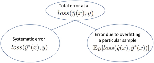
Let $y$ be the true label of an instance $x$, $\hat{y}(x)$ is the prediction at $x$.⁶ The loss at $x$ is expressed by $loss(\hat{y}(x),y)$. To begin with, the systematic prediction at $x$, ${\hat{y}}^{\ast }(x)$ is defined as the prediction that minimizes the expected loss between it and the predictions using other samples. Concretely, ${\hat{y}}^{\ast }(x)=arg{min}_{{\hat{y}}^{\prime }(x)}{\mathbb{E}}_{\mathcal{D}}[loss({\hat{y}}^{\prime }(x),\hat{y}(x))]$. Assuming that the irreducible error (aka Bayes’ error rate) is absent, this loss has two components: (1) the systematic error, i.e., the error due to the limitation of expressiveness of the model itself, which is denoted by $loss({\hat{y}}^{\ast }(x),y)$ (i.e., bias of the learner), and (2) the error due to sampling variation which is denoted by ${\mathbb{E}}_{\mathcal{D}}[loss(\hat{y}(x),{\hat{y}}^{\ast }(x))]$ (i.e., the variance of the learner). Figure 1 depicts the scenario.⁷ In order to compute the bias and variance for the ranking problem, we need to instantiate these two losses in the context of ranking error. The forms of these loss functions depend on the assumption on the form of $x$ which is described below.

Figure 1. Different types of errors for a generic loss function.

Two representations of queries. In a listwise setting a query is considered to be an instance (as opposed to individual query-document pairs). There are two ways to represent a query:

1. Permutations of documents.

2. Labels of documents.

These two representations lead to different instantiations of various quantities mentioned above. These are described below.

5.3.3. Bias-variance using permutations of documents

Suppose $\pi ({\vec{l}}_q)$ is a true ranking⁸ of the feature vectors corresponding to the documents associated with query $q$, and $\pi (\vec{f}(x_q))$ is the ranking of those documents induced by the scores predicted by the ranking model $f(.)$ learnt using a sample.⁹ Within this setting, the true label is denoted by $\pi ({\vec{l}}_q)$, the predicted label is denoted by $\pi (\vec{f}(x_q))$, and the systematic prediction for an instance is denoted by ${\mathbb{E}}_{\mathcal{D}}[\pi ({\vec{f}}_{\mathcal{D}}(x_q))]$ where $\pi ({\vec{f}}_{\mathcal{D}}(x_q))$ is the predicted ranked list of query $q$ by model $f$ learnt from dataset $\mathcal{D}$. (Note that to keep our notations simpler, we use $\vec{f}(x_q)$ to mean ${\vec{f}}_{\mathcal{D}}(x_q)$ when the meaning is obvious.)

As such, the ranking loss at a query $q$ is written as:

(9) $Er{r}_{ranking}(q)=loss(\pi (\vec{f}(x_q)),\pi ({\vec{l}}_q)).$(9)

In order to define the bias and the variance for the ranking loss, we now need to (1) define the systematic prediction, i.e., a method for aggregating multiple ranked lists, and (2) measure the amount of deviation between two ranked lists of documents. To achieve the former of these two tasks, the rank-aggregation methods such as Borda’s method can be used (Dwork et al. 2001; Sculley 2007), whereas to accomplish the latter, the well-known rank-distance methods such as Kendall’s Tau (Lapata 2006) or Spearman’s Footrule Footrule (Diaconis and Graham 1977) can be used.¹⁰ (Table 1 summarizes various quantities within this setting.) However, in what follows, we argue that using these methods, i.e., the rank aggregation and rank distance methods may not serve our purpose of measuring the variance and bias of a model in terms of ranking error.

Table 1. Using permutations of documents, instantiations of different quantities

Quantity	Instantiation
True label, $y$	$\pi ({\vec{l}}_q)$
Predicted label of a model, $\hat{y}(x)$	$\pi (\vec{f}(x_q))$
Systematic prediction, ${\hat{y}}^{\ast }(x)$	${\mathbb{E}}_{\mathcal{D}}[\pi ({\vec{f}}_{\mathcal{D}}(x_q))]$
Bias/systematic error, $loss({\hat{y}}^{\ast }(x),y)$	$rank\mathrm{\_}distance({\mathbb{E}}_{\mathcal{D}}[\pi ({\vec{f}}_{\mathcal{D}}(x_q))],\pi ({\vec{l}}_q))$
Variance, ${\mathbb{E}}_{\mathcal{D}}[loss(\hat{y}(x),{\hat{y}}^{\ast }(x))]$	${\mathbb{E}}_{\mathcal{D}}[rank\mathrm{\_}distance(\pi (\vec{f}(x_q)),{\mathbb{E}}_{\mathcal{D}}[\pi ({\vec{f}}_{\mathcal{D}}(x_q))])]$

The bias and variance should reflect the error induced by an evaluation metric that befits the problem at hand (which is, in our case, the IR ranking problem). In IR community, the nearly-ubiquitous practice regarding evaluation of a candidate ranked list of documents produced by an IR system against a gold-standard ranked list is to use a metric that incorporates per-document relevance judgments. For example, Moffat (2013) studies thirteen IR metrics that have been heavily used within the IR community (later Jones et al. (2015), among others, also conduct such a study), and all of these metrics invariably exploit the relevance judgments of individual documents in their definitions. In contrast, Kendall’s tau and other similar rank-distance metrics are popular choices in other domains of IR such as measuring the effectiveness of IR metrics (Carterette 2009; Yilmaz, Aslam, and Robertson 2008) and deciding whether two test collections are equivalent (Voorhees 2000).

Now the question is, why not use the rank-distance and aggregation metrics instead of IR metrics?¹¹ We argue that the IR researchers have not adapted rank-distance and rank-aggregation measures for IR evaluation due to the following reasons. The rank-distance and rank-aggregation metrics usually assume that every pair of items in a ranked list has a preference relationship. This, however, does not reflect the practice of IR ranking domain because conventionally only a few distinct labels are assigned to a large number of documents; thus in IR ranking there is no preference relationship in a large number of document pairs (pertaining to a query). Regarding the rank-aggregation methods, due to the same reason, to make a gold standard list of documents, an exponentially large number of candidate lists need to be aggregated, which is not going to be computationally feasible.¹² In contrast, the conventional IR metrics (e.g., DCG) represent many equivalent ranked lists by a single value, whereas the rank-aggregation metrics find it difficult (due to an exponentially large number of candidate lists and/or the heuristic nature of the algorithm) to combine many equivalent lists. Figure 2 illustrates the simplicity of IR metrics over the rank-distance and rank-aggregation metrics in evaluating the quality of a candidate ranked list of documents produced by an IR system. The left and right parts of this figure demonstrate the process of measurement of quality of a ranked list using IR metrics and rank-distance metrics respectively. In the left figure, a perfect ranked list can be arbitrarily chosen from many available ones, and then its score and the candidate ranked list’s score are compared with a special emphasis on the top portion of the list. In the right figure, many available perfect ranked lists are first aggregated to produce a single “perfect” ranked list which is then compared to the candidate list with no emphasis on the top portion of the list.

Figure 2. Pictorial view of the process of evaluating a candidate ranked list: comparison between the conventional IR metrics (left figure) and the rank-aggregation metrics (right figure).

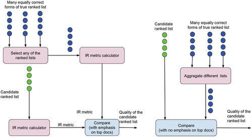
In addition, neither the rank-distance nor the rank aggregation methods usually emphasize on the top portion of a ranked list. While some rank-distance metrics such as Kendall’s tau can incorporate positional weight (Yilmaz, Aslam, and Robertson 2008), it is not immediately clear as to how these metrics relate to the conventional IR metrics such as NDCG, and we have not found any such study in the literature. In contrast, IR metrics such as DCG has a plethora of such studies (Al-Maskari, Sanderson, and Clough (2007); Sanderson et al. (2010), – to cite a few) which validate the efficacy of these metrics by taking real user satisfaction into account.

In essence, due to the mismatch between the IR evaluation approach and the rank-distance and rank-aggregation based (hypothetical) evaluation approach, we believe that using the rank-distance and aggregation metrics to define bias and variance (in terms of ranking error) may not reflect the true characteristics of bias and variance in the IR ranking domain. We, therefore, believe that using the IR evaluation metrics, which exploit relevance judgments of individual documents for bias and variance formulations, of ranking problem would be more appropriate. That said, analyzing bias and variance using the rank-distance and rank-aggregation methods is an interesting research direction that may be investigated by the researchers.

A question that may be asked: why is the above-discussed dificulty not present in the regression domain? The answer is, in the regression problem the deviation of a predicted label from the ground-truth label is well-defined (i.e., the algebraic difference), and so is the method of aggregating multiple predictions (i.e., the arithmetic mean). That is why the bias-variance decomposition of squared loss function is comparatively easier. In ranking, however, both of these two procedures are complicated.

5.3.4. Bias-variance using the dissimilarity between score lists

We now introduce the second method of estimating bias and variance that make direct use of the document labels instead of using the permutations of documents. We consider two variations in this setting: (a) using the score lists, and (b) directly using IR metrics. These two settings are described in this and next subsection respectively.

In IR ranking, the training set consists of a set of queries, $\mathcal{Q}$. Hence for a query (and associated documents), the loss can be defined as the deviation between the list of scores predicted by a model and the corresponding list of ground truth labels of the said documents. Within this setting, the true label, the predicted label and the systematic prediction for an instance is denoted by ${\vec{l}}_q$, $\vec{f}(x_q)$, and ${\mathbb{E}}_{\mathcal{D}}[{\vec{f}}_{\mathcal{D}}(x_q)]$ respectively, where ${\vec{f}}_{\mathcal{D}}(x_q)$ is the score list of query, $q$ predicted by model, $f$ learnt from dataset, $\mathcal{D}$.

As such, the ranking loss at a query $q$ can be written as:

(10) $Er{r}_{ranking}(q)=loss(\vec{f}(x_q),{\vec{l}}_q).$(10)

To define the systematic prediction, the scores $\vec{f}(x_q)$ across different samples could be averaged. To measure the $loss(.)$ between two score lists, reciprocal (or inverted) values of the standard correlation methods such as Spearnman’s correlation coefficient can then be used. Table 2 summarizes various quantities within this setting. This could be called as hybrid analysis as it incorporates both pointwise and listwise information. However, this approach has the following few problems. (1) This approach is confined to only pointwise rank-learners since the listwise algorithms do not necessarily estimate the individual relevance judgments, but rather the entire ranked lists. (2) Even when using pointwise algorithms, the limitations of pointwise analysis are also present here (of course, in a lesser degree) because of using (limited) listwise information. For example, here the variance measurement measures the fluctuation in individual scores of documents (of a particular query), but we are actually interested in measuring the variability in predictions in terms of IR evaluation metrics. For these reasons we do not recommend this setting.

Table 2. Using score lists of documents, instantiations of different quantities

Quantity	Instantiation
True label, $y$	${\vec{l}}_q$
Predicted label of a model, $\hat{y}(x)$	$\vec{f}(x_q)$
Systematic prediction, ${\hat{y}}^{\ast }(x)$	${\mathbb{E}}_{\mathcal{D}}[{\vec{f}}_{\mathcal{D}}(x_q)]$
$loss({\hat{y}}^{\ast }(x),y)$	$score\mathrm{\_}distance({\mathbb{E}}_{\mathcal{D}}[{\vec{f}}_{\mathcal{D}}(x_q)],{\vec{l}}_q)$
$loss(\hat{y}(x),{\hat{y}}^{\ast }(x))$	$score\mathrm{\_}distance(\vec{f}(x_q),{\mathbb{E}}_{\mathcal{D}}[{\vec{f}}_{\mathcal{D}}(x_q)])$

5.3.5. Bias-variance using an IR metric-based loss

In the previous two subsections we have argued that the very (IR) metrics used in evaluating a ranked list of documents should be taken into account when measuring the bias or systematic ranking error and the variability in predictions in terms of ranking error of an model. To this end, we propose that in order to measure the deviation of one ranked list from another, we make direct use of an IR metric such as NDCG as detailed below.

Like the previous setting, here the true label, the predicted label and the systematic prediction for an instance is denoted by ${\vec{l}}_q$, $\vec{f}(x_q)$, and ${\mathbb{E}}_{\mathcal{D}}[{\vec{f}}_{\mathcal{D}}(x_q)]$ respectively.

Within this setting, since the maximum possible NDCG for a query is 1, the ranking loss at query $q$ takes the following form:

(11) $Er{r}_{ranking}(q)=loss(1,NDCG({\vec{l}}_q;\vec{f}))=1-NDCG({\vec{l}}_q;\vec{f}).$(11)

We now estimate the bias or systematic ranking error at a query, $q$ as the difference between 1 (i.e., the maximum possible NDCG) and the NDCG of the document list ordered by the scores of the systematic prediction (i.e., $\bar{f}(x_q)={\mathbb{E}}_{\mathcal{D}}[{\vec{f}}_{\mathcal{D}}(x_q)]$). As such, the systematic ranking error (SRE) or the bias of a rank-learner at a query $q$ becomes:

(12) $SRE(q)=1-NDCG({\vec{l}}_q;\bar{f}).$(12)

We could then estimate the error due to variability in rank-predictions (i.e., the expected value of the “remaining error” over all possible models built on different training samples of a fixed size) at a query $q$ as: $VRE(q)={\mathbb{E}}_{\mathcal{D}}[NDCG({\vec{l}}_q;\bar{f})-NDCG({\vec{l}}_q;{\vec{f}}_{\mathcal{D}})]$, where VRE denotes the variability in predictions in terms of ranking error. The assumption behind this variance definition is that the ranking error for a query 1 – $NDCG({\vec{l}}_q;{\vec{f}}_{\mathcal{D}})$ is decomposed into bias plus variance, i.e., adding the terms SRE(q) and VRE(q) gives the expected error at a query which is ${\mathbb{E}}_{\mathcal{D}}[1-NDCG({\vec{l}}_q;{\vec{f}}_{\mathcal{D}})]$.¹³ However, a drawback of this variance definition is that the variance for a query may be systematically underestimated since for some datasets (over which the Expectation is being performed) this difference could be negative; because it may happen that the $NDCG({\vec{l}}_q;{\vec{f}}_{\mathcal{D}})$ value for a particular training dataset $D_i$ (out of the many which are used in the procedure of estimating bias and variance) is higher than $NDCG({\vec{l}}_q;\bar{f})$.

To circumvent this drawback, it would be tempting to define the variance as the squared (or absolute) difference between the NDCG of the systematic prediction and the prediction of an individual model, expected over the samples, i.e., as: $VRE(q)={\mathbb{E}}_{\mathcal{D}}[(NDCG({\vec{l}}_q;{\vec{f}}_{\mathcal{D}})-NDCG({\vec{l}}_q;\bar{f}){)}^2]$, or, alternatively, $VRE(q)={\mathbb{E}}_{\mathcal{D}}[|NDCG({\vec{l}}_q;{\vec{f}}_{\mathcal{D}})-NDCG({\vec{l}}_q;\bar{f})|]$. Doing so, however, would exacerbate the problem since it would turn any negative cost into a positive one. Elaborately, as mentioned in the previous paragraph that it may happen that the $NDCG({\vec{l}}_q;{\vec{f}}_{\mathcal{D}})$ of a particular sample is higher than $NDCG({\vec{l}}_q;\bar{f})$. This means that this incident of observing a higher $NDCG({\vec{l}}_q;{\vec{f}}_{\mathcal{D}})$ is a positive outcome, but the above-mentioned formulae consider it as an error component by adding the (squared or absolute) difference between $NDCG({\vec{l}}_q;{\vec{f}}_{\mathcal{D}})$ and $NDCG({\vec{l}}_q;{\vec{f}}_{\mathcal{D}})$ in the variance calculation.¹⁴ Considering this problem, we propose a definition for the error due to variability in rank-prediction at a query $q$ as follows:

(13) $VRE(q)={\mathbb{E}}_{\mathcal{D}}[|NDCG({\vec{l}}_q;\bar{f})-NDC{G}_{f_{\mathcal{D}}}({\vec{l}}_q;{\vec{f}}_{\mathcal{D}}){|}_{+}],$(13)

where $|a{|}_{+}$ denotes the positive only, i.e., $|a{|}_{+}=max(0,a)$.

It is evident from this definition that the problems of the previous two definitions (cf. Tables 1 and 2) are not present here. However, the ranking loss here is no longer assumed to be decomposable into the bias and variance (because of the $|.{|}_{+}$ operator). Nonetheless, this definition is close to the additive decomposition of ranking error.

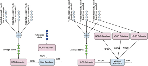
Table 3 summarizes the various quantities defined according to the above-mentioned discussion. Figure 3 illustrates the instantiations of two types of losses in ranking domain. Figure 4 illustrates the procedure for computing SRE and VRE for a query.

Table 3. Using IR metrics on score lists of documents, instantiations of different quantities

Quantity	Instantiation
True label, $y$	${\vec{l}}_q$
Predicted label of a model, ${\hat{y}}^{(}x)$	$\vec{f}(x_q)$
Systematic prediction, ${\hat{y}}^{\ast }(x)$	${\mathbb{E}}_{\mathcal{D}}[{\vec{f}}_{\mathcal{D}}(x_q)]$
$loss({\hat{y}}^{\ast }(x),y)$	$1-NDCG({\vec{l}}_q;{\mathbb{E}}_{\mathcal{D}}[{\vec{f}}_{\mathcal{D}}(x_q)])$
$loss(\hat{y}(x),{\hat{y}}^{\ast }(x))$	$|NDCG({\vec{l}}_q;{\mathbb{E}}_{\mathcal{D}}[{\vec{f}}_{\mathcal{D}}(x_q)])-NDCG({\vec{l}}_q);\vec{f}(x_q){|}_{+}$

Figure 3. Bias and variance estimation for ranking error.

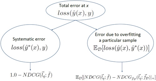
Figure 4. Pictorial view of the process of calculation of systematic ranking error (SRE) (left figure) and variability in predictions in terms of ranking error (VRE) (right figure) for a query (using different samples).

It is plausible that the approach of estimating the bias using SRE and the variance using VRE outlined above is able to analyze the systematic error and the error due to variability in prediction of a model in terms of ranking error. However, this setting has a problem from theoretical perspective: according to the desiderata listed by Kohavi and Wolpert et al. (1996), for a generic loss function, a definition of variance must be independent of the ground truth labels (later on, James (2003) suggested similar properties). In contrast, our variance definition (Equation 13(13) $VRE(q)={\mathbb{E}}_{\mathcal{D}}[|NDCG({\vec{l}}_q;\bar{f})-NDC{G}_{f_{\mathcal{D}}}({\vec{l}}_q;{\vec{f}}_{\mathcal{D}}){|}_{+}],$(13) ) makes use of ground truth labels. This problem, however, is difficult to avoid as it has been discussed earlier that almost all of the IR metrics make direct use of relevance labels for documents. Apart from this caveat, this framework essentially avoids the problems of the previously discussed approaches outlined in Sections 5.3.3 and 5.3.4. Using this framework we are able to measure the systematic ranking error of a rank-learner across the different training sets (i.e., bias) and the ranking error that results from the variation in predictions across the different training sets (conceptually similar to the variance).

An important merit of our framework developed in this section is that it is applicable to all types of LtR algorithms (pointwise, listwise etc.).

We discussed in Section 4 that to the best of our knowledge there is no investigation in the literature into decomposition of bias and variance for ranking error. The loss function of squared error has nice mathematical properties (which are mostly absent in the zero-one loss function of classification) that make it easy to decompose. For the classification problem which is a mature field of research, there is a multitude of decompositions and some of them are somewhat contradictory to one another (Domingos 2000). We have argued that the true loss function of ranking problem is even more complicated since it involves a group of instances (documents) and also the scores themselves are not the main targets for prediction. While we have argued that the framework presented above is capable of estimating the bias and variance of ranking error, it still remains an open question that how exactly the bias and variance decompose.

5.3.6. Formulae for estimating listwise bias and variance

In this section we describe the exact formulae that we use for estimating VRE and SRE.

Estimating quantities using bootstrap samples

As was the case for the pointwise analysis, we estimate SRE and VRE using two methods: (1) bootstrap samples (this subsection), and (2) repeated twofold cross-validation (the next subsection). In this subsection, we assume that $B$ bootstrap samples (without replacement) $\{{\mathcal{D}}_1,{\mathcal{D}}_2,\dots ,{\mathcal{D}}_B\}$ are generated from the original training set $\mathcal{D}$.

Systematic Ranking Error (SRE): $SRE(q)$ is measured as the difference between 1 and the ranking performance of the systematic predictions. Concretely:

(14) $\hat{S}R{E}_{bootstrap}=\frac{1}{\left|\mathcal{Q}\right|}\sum _{l=1}^{\left|\mathcal{Q}\right|}\hat{S}R{E}_{bootstrap}{\left(q_l\right)}^{\hspace{0.17em}}$(14)

$\mathrm{w}\mathrm{h}\mathrm{e}\mathrm{r}\mathrm{e}\hat{S}R{E}_{bootstrap}(q_l)=(1-NDCG(q_l;\bar{f})),$

where $NDCG(q_l;\bar{f})$ is calculated on the list ranked by the average scores across all $B$ learners (built from samples ${\mathcal{D}}_i,1\le i\le B$), i.e., by $\bar{f}(q_l)=\frac{1}{B}{\sum }_{i=1}^B{\vec{f}}_{{\mathcal{D}}_i}(q_l)$.

Variability in Rank-prediction Error (VRE): VRE of a ranking algorithm is estimated by averaging $VRE(q)$ values over all queries.

$VRE$ for a query is estimated as the positive differences between the ranking performance of systematic prediction and the ranking performance of the individual models, averaged over multiple models. Concretely:

$\hat{V}R{E}_{bootstrap}(q_l)=\frac{1}{B-1}\sum _{i=1}^B|NDCG(q_l;\bar{f})-NDCG(q_l;{\vec{f}}_{{\mathcal{D}}_i}){|}_{+},$

where $|a{|}_{+}=max(0,a)$, and $NDCG(q_l;{\vec{f}}_{{\mathcal{D}}_i})$ is value for query $q_l$ computed from the prediction of $i$ th model.

Finally:

(15) $\hat{V}R{E}_{bootstrap}1mu=1mu\frac{1}{\left|\mathcal{Q}\right|}1mu\sum _{l=1}^{\left|\mathcal{Q}\right|}\hat{V}R{E}_{bootstrap}\left(q_l\right)$(15)

Estimating quantities using repeated two-fold cross-validation

Recall that within this setting we generate two disjoint training sets ${\mathcal{D}}_1$ and ${\mathcal{D}}_2$ from the original set $\mathcal{D}$, and we repeat this process $J$ times that results in samples

$\{{\mathcal{D}}_{11},{\mathcal{D}}_{21},{\mathcal{D}}_{12},{\mathcal{D}}_{22},\dots ,{\mathcal{D}}_{1J},{\mathcal{D}}_{2J}\}$ where ${\mathcal{D}}_{1j}\cap {\mathcal{D}}_{2j}=\mathrm{\varnothing }$.

Systematic Ranking Error (SRE): With $1\le j\le J$, the $j$ th estimate of SRE of the model is calculated as:

$\hat{S}R{E}_{twofol{d}_j}1mu=1mu\frac{1}{\left|\mathcal{Q}\right|}1mu\sum _{l=1}^{\left|\mathcal{Q}\right|}\hat{S}R{E}_{twofol{d}_j}\left(q_l\right)$

$\mathrm{w}\mathrm{h}\mathrm{e}\mathrm{r}\mathrm{e}\hat{S}R{E}_{twofol{d}_j}\left(q_l\right)=\left(1-NDCG\left(q_l;{\bar{f}}_j\right)\right),$

where ${\bar{f}}_j(q_l)=\frac{1}{2}{\sum }_{i=1}^2{\vec{f}}_{{\mathcal{D}}_{ij}}(q_l)$.

Finally:

(16) $\hat{S}R{E}_{twofold}=\frac{1}{J}\sum _{j=1}^J\hat{S}R{E}_{twofol{d}_j}.$(16)

Variability in Ranking Error (VRE): The $j$ th estimate for $VRE$ of the model is given by:

$\hat{V}R{E}_{twofol{d}_j}1mu=1mu\frac{1}{\left|\mathcal{Q}\right|}1mu\sum _{l=1}^{\left|\mathcal{Q}\right|}\hat{V}R{E}_{twofol{d}_j}\left(q_l\right)$

where,

$\hat{V}R{E}_{twofol{d}_j}(q_l)=\frac{1}{2-1}\sum _{i=1}^2|NDCG(q_l;{\bar{f}}_j)-NDCG(q_l;{\vec{f}}_{{\mathcal{D}}_{ij}}){|}_{+}.$

Finally:

(17) $\hat{V}R{E}_{twofold}=\frac{1}{J}\sum _{j=1}^J\hat{V}R{E}_{twofol{d}_j}.$(17)

An important property of our proposed framework is that it is generic i.e. algorithm-independent and easy to employ. One simply needs to compute, for the LtR algorithm in question, the quantities in Equations 5(5) ${\hat{b}}_{bootstrap}^2=\frac{1}{N}\sum _{k=1}^N{\hat{b}}_{bootstrap}^2(x_k),$(5) , 6(6) ${\hat{\sigma }}_{bootstrap}^2=\frac{1}{N}\sum _{k=1}^N{\hat{\sigma }}_{bootstrap}^2(x_k)$(6) (pointwise, method of bootstrapping), 7, 8 (pointwise, method of repeated twofold), 14, 15 (listwise, method of bootstrapping), 16, 17 (listwise, method of repeated twofold) and examine their behavior as one varies a parameter of the algorithm. In doing so insight will be gained about the strength and weakness of the algorithm in terms of bias and variance.

6. Empirical evaluation

In the previous part of this article we have developed a framework for computing bias and variance of rank-learners. Although the nature of this article is mainly theoretical, it is always useful to examine how theories work in practice. We therefore turn our attention to an empirical evaluation of our proposed framework.

6.1. Random forest and learning-to-rank

In perhaps the most prominent LtR challenge (Chapelle and Chang 2011) it is observed that the tree-ensemble based algorithms usually outperform others. Such a model utilizes a collage of classification/regression trees to predict the relevance score of a document with respect to a query.¹⁵ Mainly two types of ensembles have been found so far to be effective in LtR literature: random forest (Breiman 2001) and gradient boosting (Friedman 2001). Random forest based algorithms have recently been shown to be on a par with its gradient boosting counterparts (Ibrahim 2020). To avoid overstretching the article, we confine our experiments on mainly random forest based LtR algorithms, although we do perform some experiments on a gradient-boosting based LtR algorithm as well.

A random forest is a conceptually simple but effective and efficient learning algorithm that aggregates the outputs of a large number of independent and variant base learners, usually decision trees. It is an (usually bagged) ensemble of recursive partitions over the feature space, where each partition is assigned a particular class label (for classification) or a real number (for regression), and where the partitions are randomly chosen from a distribution biased toward those giving the best prediction accuracy. For classification the majority class within each partition in the training data is usually assigned to the partition, while for regression the average label is usually chosen, so as to minimize zero-one loss and mean squared error respectively. In order to build the recursive partitions, a fixed-sized subset of the attributes is randomly chosen at each node of a tree, and then for each attribute the training data (at that node) is sorted according to the attribute and a list of potential split-points (midpoints between consecutive training datapoints) is enumerated to find the split which minimizes expected loss over the child nodes. Finally the attribute and associated split-point with the minimal loss is chosen and the process is repeated recursively down the tree. For classification the entropy or gini function¹⁶ is used to calculate the loss for each split, while for regression the mean squared error is used (Ibrahim and Carman 2016).

Random forests have been adapted to solve the LtR problem from pointwise (Mohan, Chen, and Weinberger 2011), (Geurts and Louppe 2011), pairwise and listwise perspectives (Ibrahim 2020).

6.1.1. Random forest-based LtR

In the experiments that follow, we mainly use an RF based pointwise rank-learner with regression setting (denoted by simply RF-point). However, as mentioned earlier, our proposed framework of pointwise analysis are applicable to any pointwise rank-learner, and the framework of listwise analysis are applicable to any (pointwise/pairwise/listwise) rank-learner. RF-point algorithm uses the regression setting that treats the relevance judgments (for example, from 0 up to 4) as target variables, and then minimizes the sum of squared error over the data at a node of a tree during a split. The documents are finally sorted in decreasing order of their predicted scores to produce a ranking. For a detailed description of the algorithm, please see Ibrahim (2020). We apply both the pointwise and listwise settings to RF-point algorithm.

6.1.2. Effect of sub-sample size (per-tree) on bias-variance

We are going to examine how the bias and variance profiles react while varying a parameter of the learning algorithm RF-point. Ibrahim (2019) reveal that proper tuning of the sub-sample size per tree in the context of LtR may yield better accuracy and at the same time allows for scaling up the algorithm for large datasets. We take this parameter for our analysis.

In bagging (Breiman 1996) (which is known as a predecessor of a random forest), the tendency is to reduce training set similarity across different trees by using a bootstrapped sample (i.e., using around 63% data) to learn each tree. A random forest keeps the default setting of bagging with regard to the method of sampling per tree, but exploits another dimension in its favor which is the number of candidate features to consider for splitting at each node, thereby reducing variance. At an intuitive level, one might be tempted to think that a bagged ensemble, by reducing the training sample per tree further below 63%, could have achieved the same reduction of variance as achieved by a random forest. However, Friedman and Hall (2007) show that if less than 50% data are used, it does not decrease the error rate of bagging, even though it does reduce the variance (we note that reducing correlation generally increases bias and variance of individual base learners, i.e., trees). However, the effect of a random forest’s reduction of variance (by using another dimension which is the number of candidate features at each node) empirically turns out to be favorable to reducing generalization error.

Then comes the idea of Ibrahim (2019): can we achieve better performance by holding the best configuration of a random forest in terms of number of candidate features, and then by going backward to the initial motivation of bagging (which was to decrease the commonalities amongst sub-samples used to learn individual trees)? Once again, the main goal is to reduce variance (and eventually variance of ensemble of sub-sampled trees) but in a different way from both the bagging and random forest. In doing so, however, it gives rise to the risk of increasing individual tree variance and bias, thereby warranting proper tuning of the parameter.

Although there have been some work on analyzing the correlation, strength and generalization error of a random forest in the context of classification and regression (Bernard, Heutte, and Adam 2009; Lin and Jeon 2006; Segal 2004), we have not found any work on the bias-variance interaction of random forest based rank-learners. The remaining portion of this article attempts to fill this gap in the literature: in the earlier part we offered an understanding of the theory of rank-learners in terms of their bias-variance characteristics, and now we want to see how the theory applies to practice by investigating into an important parameter of the RF-based LtR algorithms, namely the sub-sample size per tree.

6.2. Datasets and experimental settings

We use two of the most widely used (big) datasets of LtR, namely MSLR-WEB10K and Yahoo because theoretical results are usually pronounced with big datasets. Table 4 shows their statistics. Further details can be found in Qin et al. (2010), in Microsoft Research website,¹⁷ and in Chapelle and Chang (2011). Both the datasets are pre-divided into three chunks: training set, validation set and test set. For the sake of better compatibility with the existing literature, the algorithms in this paper are trained using these pre-defined training sets. The features of all these datasets are mostly used in academia. However, features of the Yahoo dataset (which was published as part of a public challenge (Chapelle and Chang 2011)) are not disclosed as these are used in a commercial search engine.

Table 4. Statistics of the datasets

Characteristic	MSLR-WEB10K	Yahoo
Task	Web Search	Web Search
# Queries (overall)	10000	29921
# Queries (train)	6000	19944
# Features	136	519
# Rel. labels	5	5
# Query-doc pairs (overall)	1200192	709877
# Query-doc pairs (train)	723412	473134
# Docs per query	120	23
# Docs of diff.	2/39/16/2/0.9	6/8/7/2/0.4
labels (0/1/2/3/4) per query

As evaluation metrics, we use two widely known measures, namely NDCG@10 and MAP.¹⁸ In the results that follow, for the method of bootstrapping we use $B=10$ and for the method of repeated twofold CV we use $J=5$. The ensemble size, i.e., the number of trees in an RF is 500, and unpruned trees are learnt.

As mentioned in Section 6.1.1, as the learning model, in this section we use RF-point algorithm.

6.3. Result analysis: Pointwise setting

This section analyzes the plots of bias and variance estimated using the pointwise analysis. Figure 5 shows the plots for the method of bootstrapping and repeated twofold CV.¹⁹

Figure 5. Pointwise analysis with both the methods of bootstrapping and repeated twofold CV: ensemble bias and ensemble variance estimates on MSLR-WEB10K (top row) and Yahoo (bottom row) datasets with RF-point (regression setting).

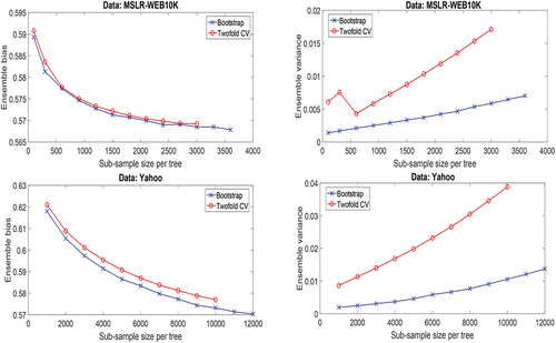
The trends of the plots of MSLR-WEB10K and Yahoo datasets are largely similar to each other. They are also similar across the method of bootstrapping and method of repeated twofold CV, which implies that both the methods are effective to capture the trend of bias and variance.

Broadly, for both the datasets the plots corroborate our hypothesis mentioned earlier which was the bias and variance would trade-off while the sub-sample size per tree, $p$ is increased.

As for the ensemble variance, increasing $p$ (which decreases the individual tree variances) does not necessarily translate into decreased ensemble variance because besides the single tree variance the correlation is the other factor in deciding the ensemble variance.²⁰ It is due to the increased correlation the ensemble variance keeps on increasing as we increase the sub-sample size per tree.

We know that the bias does not depend on the peculiarities of the training set, whereas the variance does. Given that the training set sizes in both the methods of bootstrap and repeated twofold CV are sufficiently close to each other (containing approximately 63% and 50% of original sample respectively), the bias in both the methods has been found to be of similar absolute values (from $\approx$ 0.56 to $\approx$ 0.6). The small changes in bias across the two methods are likely due to the randomness and small change in training set size. But the variances do differ greatly ($\approx$ 3.5 times for the last configurations), and the difference is according to our conjecture made earlier which was, the variance estimate of method of repeated twofold CV is greater than that of method of bootstrapping as the former’s training sets are disjoint whereas the latter’s are not. The increasing trend of the variance estimates, however, is captured by both the methods, which implies that any of the two methods can be used to visualize the trend.

The ensemble variance with very small $p$ is still quite small which may seem to be counter-intuitive. Wager, Hastie, and Efron (2014) show for a regression dataset that reducing the correlation greatly (by using a very small feature set for each split, $K$) causes high ensemble variance. The apparent discrepancy between their findings and ours can be explained by the fact that they used a quite smaller dataset (20640 instances and 8 features) whereas the minimum configuration of our setting uses 5% queries per tree which is 300 queries for MSLR-WEB10K (with 120 documents per query) and 23000 queries for Yahoo datasets (with 23 documents per query), and 136 and 519 features respectively. Hence in our case reducing the sample size per tree does not heavily increase the individual tree variances, thereby resulting in comparatively low ensemble variance. In contrast, in their study, when they drastically reduce $K$, the reduction in correlation alone cannot limit the significantly higher individual tree variance, thereby resulting in higher ensemble variance.

6.4. Result analysis: Listwise setting

This section analyzes plots of SRE and VRE quantities. In Figure 6 we see that the trends of the plots are according to our conjecture which is the variance and bias trade-off with increasing sub-sample size per tree, which corroborates that our formulations for analyzing bias and variance of ranking error (SRE and VRE) are indeed reliable.

Figure 6. Listwise analysis with both the methods of bootstrapping and repeated twofold CV: ensemble bias and ensemble variance estimates on MSLR-WEB10K (top row) and Yahoo (bottom row) datasets with RF-point (regression setting).

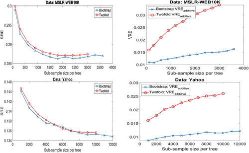
Also, like the pointwise analysis, the trends of the plots of method of repeated twofold CV are similar to that of method of bootstrapping. The absolute values of SRE are similar across different methods, which is expected. The values of VRE estimates of method of bootstrapping are less than that of method of repeated twofold CV, which is also expected. The value of SRE on Yahoo dataset is less than that on MSLR-WEB10K (approximately half). The VRE, however, maintains comparable values across the two datasets.

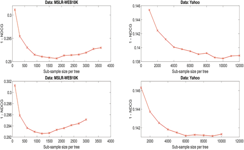
On the MSLR-WEB10K, SRE appears to flatten off and even increase slightly for large values of $p$. However, in the pointwise analysis (cf. Figure 5) the bias was found to be ever-decreasing with increasing $p$, which means that the scores of individual documents, on average, are better predicted with increasing $p$. A possible explanation for this apparently different findings is that although the optimal (minimal) mean-squared error results in optimal (maximal) NDCG, but it is not necessarily the case that reducing mean-squared error will always increase NDCG. An example of this is simple to imagine. Another perspective for explaining this slightly increasing trend of SRE on MSLR dataset is that the error rate heavily depends on SRE (since VRE is quite small), so the trend of the SRE curve almost mimics the ranking error curve (cf. Figure 7).

Figure 7. Ranking error with the methods of bootstrapping (top row) and repeated twofold CV (bottom row).

6.5. Listwise bias and variance comparison of multiple algorithms

In the previous subsections we have used a single LtR algorithm to study its bias and variance trends while we have varied a parameter of the algorithm. Analyzing bias and variance has another important use which is to compare the relative performance of various algorithms with an aim to see which algorithm is mostly affected by which of these two quantities. In doing so, the practitioners will be able to improve that specific quantity instead of trying arbitrary options. Now we conduct such a pilot comparative study using two LtR algorithms, namely RF-point and LambdaMart algorithms, using the SRE and VRE estimates. LambdaMart (Wu et al. 2010) is one of the most popular LtR algorithms. It blends the ingenuine idea of approximated gradient of its predecessor, namely LambdaRank (Quoc and Le 2007) with the gradient boosting framework (Friedman 2001).²¹

We compute SRE and VRE using the method of repeated twofold CV on MSLR-WEB10K and Yahoo datasets – we preferred the method of repeated twofold CV because LambdaMart is a deterministic algorithm, so using the method of bootstrapping (which uses overlapped samples) might greatly underestimate the variance of LambdaMart.

Table 5 shows the results. We see that on both the datasets for both the algorithms, SRE is the main contributor to the error rate. However, this does not necessarily mean that VRE is unimportant because on Yahoo dataset the SRE of LambdaMart is higher than that of RF-point, but due to the opposite trend in VRE, the error rate of LambdaMart is lower than that of RF-point.

Table 5. Comparison between RF-point (RF-p) and LambdaMart (LMart) using SRE and VRE on MSLR-WEB10K (fold 1) and Yahoo datasets

Data: MSLR-WEB10K
1-NDCG	1-NDCG	$SRE$		$VRE$
RF-p	LMart	RF-p	LMart	RF-p	LMart
0.2931	0.2954	0.2871	0.2895	0.0294	0.0300
Data: Yahoo
1-NDCG	1-NDCG	$SRE$		$VRE$
RF-p	LMart	RF-p	LMart	RF-p	LMart
0.1406	0.1396	0.1366	0.1374	0.0215	0.0192

Now, what recommendations can we offer for practitioners from all these experiments? Brain and Webb (2002) advocate for designing learning algorithms that meet the specific need of the dataset at hand in terms of bias and variance. For example, we conjecture that for big datasets variance reduction may not need to be the key target of the rank-learning algorithms. Indeed, in our experiments the value of SRE has been found to be far greater than VRE which implies that SRE is the main contributor to the ranking error rather than VRE. Following this motivation, some researchers focus on reducing either bias (Zhang and Lu 2012), (Ghosal and Hooker 2020) or variance (Horváth et al. 2021) of an algorithm that is known to have a high value of the respective quantity. Currently we have not found any LtR algorithm that aims to improve ranking accuracy guided by the bias-variance analysis. From this study we promote this very idea. That is, after computing SRE and VRE quantities of a dataset, practitioners will be able to focus on reducing either bias or variance or both in an informed and guided way. This study recommends that LtR practitioners should follow the standard procedure of machine learning discipline for error mitigation: they should compute the bias and variance of the algorithm of their choice and then engineer the system (i.e., either improve the data or the hypothesis space or both) according to the findings of bias-variance analysis.

7. Conclusion

This paper presents what we believe to be the first thorough study about the bias-variance analysis of learning-to-rank algorithms. We have thoroughly discussed various potential definitions of bias and variance for the ranking problem in information retrieval. We have formulated the bias and variance from both pointwise and listwise perspective. We have also demonstrated how exactly to calculate these quantities using a training sample. The developed framework is readily-available for being employed to study the relative strengths and weaknesses of various LtR algorithms with an aim to analyze their bias and variance tradeoff.

Our formulations of bias and variance have been found to be working well in practice as we, when working with the random forest based rank-learners, observed the classical bias-variance tradeoff while varying the parameter sub-sample size per tree. We have also shed some light on relative performance of two widely used rank-learning algorithms. The methodology of bias and variance analysis proposed in this paper can directly be applied to all types of rank-learning algorithms irrespective of their loss functions.

Being the first thorough study on bias and variance of rank-learners, this work puts forth a number of intriguing research directions which are as follows. Given that the absolute values of bias differs in the two investigated datasets, an interesting research direction would be to investigate what aspects of a dataset causes an learning-to-rank algorithm to have higher/lower bias and variance. Another attracting direction for future research would be to investigate alternative definitions of listwise bias and variance and decompositions of ranking error as indicated in Section 5.3.3. Yet another direction for future work would be to conduct a thorough study to explain relative performance of different LtR algorithms using the notions of listwise bias and variance proposed here.

Disclosure Statement

No potential conflict of interest was reported by the author(s).

Notes

1. Sometimes NDCG is truncated at a value $k\le n_q$, and is denoted by NDCG@$k$. Throughout the paper we shall use NDCG to refer to the un-truncated version.

2. Provided that the learning algorithm is consistent, this will correspond to the point of minimum loss in the parameter space.

3. In the context of LtR, this assumption implies that we are considering the relevance judgments of documents to be deterministic.

4. We note here that there is a discussion in the literature regarding casting the classification problem (with class posterior probabilities) onto regression and then using the formulations and bias-variance decomposition of regression problem such as by (Manning, Raghavan, and Schütze 2008, Sec. 14.6) and (Hastie, Tibshirani, and Friedman 2009, Sec. 15.4) – we quote the comment of the latter work: “ … Furthermore, even in the case of a classification problem, we can consider the random-forest average as an estimate of the class posterior probabilities, for which bias and variance are appropriate descriptors.” However, Friedman (1997) explains that a better calibration of the class posterior probabilities of the correct class does not necessarily translate into a higher accuracy of a classifier (in terms of 0/1 loss). A similar concern is true for ranking loss functions, hence the investigation of listwise rather than pointwise bias-variance analysis is important.

5. Hence the scores predicted by these algorithms (e.g., LambdaMart (Wu et al. 2010)) can even be negative.

6. Here $x$ is a generic instance, not necessarily the feature vector corresponding to a query-document pair.

7. The work by Domingos (2000) is useful to further understand this concept.

8. There may be more than one perfect ranking for a set of documents associated with a query.

9. The symbol $\pi$ is a bijection on the set of items $\{1,2,\dots ,n_q\}$, i.e., $\pi :\{1,2,\dots ,n_q\}\to \{1,2,\dots ,n_q\}$.

10. Borda’s count is a classic method that dates back to 17th century. It aggregates various ordered lists of a set of items to produce a single ordered list of those items. Its variations are frequently used till date. Kendall’s Tau and Spearman’s Footrule are two instances of generalized rank correlation coefficient. These metrics measure the degree of agreement (and disagreement thereof) between two ordered list of a set of items by using the number of concordant and discordant pairs and the relative positions of the items.

11. It is relatively straightforward to define an “IR evaluation metric” based on the rank-distance metrics by negating (i.e. inverting) the value of the distance between the candidate list and the gold-standard list. A single gold-standard list may be produced from many equivalent (gold-standard) lists by applying a rank-aggregation method on the equivalent lists.

12. It is known that producing an optimal aggregation, i.e., finding an aggregate list which minimizes the number of miss-ranked pairs across all candidate lists is an NP-hard problem for even only four lists (Dwork et al. 2001). (Although the limited number of distinct labels in IR domain may reduce this time complexity, the solution is not immediately clear.) Eventually heuristic algorithms are used in the literature to solve the problem which come with their own limitations.

13. A pitfall here would be to define the expected ranking loss as: $Er{r}_{ranking}(q)=(1-NDCG(q){)}^2$. At a first glance this definition may look appealing because we could use the similar derivation of the regression problem (cf. Equation 4)(4) $Er{r}_{mse}(x_k)=\mathbb{E}[(f(x_k)-l_k{)}^2]$(4) to decompose the squared bias as $(1-{\mathbb{E}}_{\mathcal{D}}[NDCG({\vec{l}}_q;{\vec{f}}_{\mathcal{D}})]{)}^2$ and variance as ${\mathbb{E}}_{\mathcal{D}}[(1-{\mathbb{E}}_{\mathcal{D}}[NDCG({\vec{l}}_q;{\vec{f}}_{\mathcal{D}})]{)}^2]$. However, this setting has a major problem: the systematic prediction, i.e., the quantity ${\mathbb{E}}_{\mathcal{D}}[NDCG({\vec{l}}_q;{\vec{f}}_{\mathcal{D}})]$ is in fact not of our interest. The reason is, ${\mathbb{E}}_{\mathcal{D}}[NDCG({\vec{l}}_q;{\vec{f}}_{\mathcal{D}})]$ (which is estimated by $\overline{NDCG}(q)=\frac{1}{N}{\sum }_{i=1}^{N}NDC{G}_i(q)$ where $N$ is the number of training samples) does not measure the average predictions of the models, but rather it simply measures the average quality of ranking performance after applying an IR evaluation measure on predictions of individual models.

14. A natural question to ask is: why is in the regression setting this phenomenon not a problem? We note that in the regression setting, predicting both the greater or less than the target value is an error. But in the ranking problem, observing a greater NDCG is always a positive outcome. Elaborately, in the regression problem, the variance estimate tells us how much variation we expect to observe when the model is learnt from a different sample. Here both the positive and negative fluctuations in predictions, i.e., both the higher and lower predictions than the true label are condemnable because the goal is to predict the exact target value. In the ranking problem, it is true that the definition ${\mathbb{E}}_{\mathcal{D}}[(NDCG({\vec{l}}_q;{\vec{f}}_{\mathcal{D}})-NDCG({\vec{l}}_q;\bar{f}{)}^2]$ of the variance estimate tells us as to how much fluctuation in predictions in terms of NDCG we expect to observe across different samples. But unlike regression, here if a particular model yields a higher NDCG than the “systematic NDCG” (i.e., $NDCG({\vec{l}}_q;\bar{f})$), this is in fact a positive outcome, so we should not consider it as an error to be contributed to the variance term.

15. Throughout the rest of the paper we use the terms ensemble and model interchangeably.

16. If $p(c|L)$ denotes the estimated probability of a class at a leaf then ${\mathcal{L}}_{entropy}\left(Lf\right)=-\sum _{c}p(c|Lf)log(p(c|Lf))$ and ${\mathcal{L}}_{gini}\left(Lf\right)=\sum _{c}p(c|Lf)(1-p(c|Lf))$

17. http://research.microsoft.com/en-us/projects/mslr/

18. To know details of these metrics, the readers are advised to go through Järvelin and Kekäläinen (2000).

19. The curves of the repeated twofold CV method stop earlier than that of the bootstrap method because in the former method the size of a training set is half of the original sample, whereas in the latter method the size of a training set is approximately two-third of the original sample.

20. Variance of a random forest is expressed as the multiplication of correlation between the trees and a single tree variance. For details, please see the Appendix section of Ibrahim (2019).

21. We use an open-source implementation of it mentioned in Ganjisaffar, Caruana, and Lopes (2011) (https://code.google.com/p/jforests/). The parameter settings that we maintain are as follows: number of trees = 500, number of leaves for each tree = 31 (Ganjisaffar et al. (2011) report that value close to this has been found to be worked well for MSLR-WEB10K).

References

- Al-Maskari, A., M. Sanderson, and P. Clough (2007). The relationship between ir effectiveness measures and user satisfaction. In Proceedings of the 30th annual international ACM SIGIR Conference on Research and Development in Information Retrieval, pp. 773–759. Amsterdam, Netherlands: ACM.
- Bernard, S., L. Heutte, and S. Adam. 2009. Towards a better understanding of random forests through the study of strength and correlation, In Emerging intelligent computing technology and applications. Berlin, Heidelberg: With Aspects of Artificial Intelligence, pp. 536–545. Springer.
- Brain, D., and G. I. Webb. 2002. The need for low bias algorithms in classification learning from large data sets. In Principles of data mining and knowledge discovery, 62–73. Berlin, Heidelberg: Springer.
- Breiman, L. 1996. Bagging predictors. Machine Learning 24 (2):123–40. doi:10.1007/BF00058655.
- Breiman, L. 2001. Random forests. Machine Learning 45 (1):5–32.
- Carterette, B. (2009). On rank correlation and the distance between rankings. In Proceedings of the 32nd international ACM SIGIR Conference on Research and Development in Information Retrieval, pp. 436–43. Boston MA, USA: ACM.
- Chapelle, O., and Y. Chang. 2011. Yahoo! learning to rank challenge overview. Journal of Machine Learning Research-Proceedings Track 14:1–24.
- Cossock, D., and T. Zhang. 2006. Subset ranking using regression 19th Annual Conference on Learning Theory 2006 (Springer) Pittsburgh PA, USA. 605–619.
- Diaconis, P., and R. L. Graham. 1977. Spearman’s footrule as a measure of disarray. Journal of the Royal Statistical Society: Series B (Methodological) 39 (2):262–68.
- Domingos, P. 2000 A unified bias-variance decomposition Proceedings of the 17th International Conference on Machine Learning (ICML). San Francisco CA: Morgan Kaufmann: Pp. 231–38.
- Dwork, C., R. Kumar, M. Naor, and D. Sivakumar (2001). Rank aggregation methods for the web. In Proceedings of the 10th International Confference on World Wide Web, Hong Kong, pp. 613–22. ACM.
- Friedman, J. H., and P. Hall. 2007. On bagging and nonlinear estimation. Journal of Statistical Planning and Inference 137 (3):669–83.
- Friedman, J. H. 1997. On bias, variance, 0/1—loss, and the curse-of-dimensionality. Data Mining and Knowledge Discovery 1 (1):55–77.
- Friedman, J. H. 2001. Greedy function approximation: A gradient boosting machine. (English summary). Annals of Statistics 29 (5):1189–232.
- Ganjisaffar, Y., R. Caruana, and C. V. Lopes (2011). Bagging gradient-boosted trees for high precision, low variance ranking models. In Proceedings of the 34th international ACM SIGIR conference on Research and development in Information Retrieval Beijing, China, pp. 85–94. ACM.
- Ganjisaffar, Y., T. Debeauvais, S. Javanmardi, R. Caruana, and C. V. Lopes (2011). Distributed tuning of machine learning algorithms using mapreduce clusters. In Proceedings of the 3rd Workshop on Large Scale Data Mining: Theory and Applications, San Diego CA, USA, pp. 2. ACM.
- Geman, S., E. Bienenstock, and R. Doursat. 1992. Neural networks and the bias/variance dilemma. Neural Computation 4 (1):1–58.
- Geurts, P., and G. Louppe (2011). Learning to rank with extremely randomized trees. In JMLR: Workshop and Conference Proceedings, Boston MA, USA, Volume 14.
- Geurts, P. 2005. Bias vs variance decomposition for regression and classification. In Data mining and knowledge discovery handbook, 749–63. Boston MA, USA: Springer.
- Ghosal, I., and G. Hooker. 2020. Boosting random forests to reduce bias; one-step boosted forest and its variance estimate. Journal of Computational and Graphical Statistics 30 (2):493–502.
- Hastie, T., R. Tibshirani, and J. Friedman (2009). The elements of statistical learning.
- Hofmann, K., S. Whiteson, and M. de Rijke. 2013. Balancing exploration and exploitation in listwise and pairwise online learning to rank for information retrieval. Information Retrieval 16 (1):63–90.
- Horváth, M. Z., M. N. Müller, M. Fischer, and M. Vechev. 2021. Boosting randomized smoothing with variance reduced classifiers. arXiv Preprint arXiv:2106 06946.
- Ibrahim, M., and M. Carman. 2016. Comparing pointwise and listwise objective functions for random-forest-based learning-to-rank. ACM Transactions on Information Systems (TOIS) 34 (4):20.
- Ibrahim, M., and M. Murshed. 2016. From tf-idf to learning-to-rank: An overview. In Handbook of research on innovations in information retrieval, analysis, and management, Martins, J. T., and Molnar, A., edited by, 62–109. USA: IGI Global.
- Ibrahim, M. 2019. Reducing correlation of random forest–based learning-to-rank algorithms using subsample size. Computational Intelligence 35 (4):774–98.
- Ibrahim, M. 2020. An empirical comparison of random forest-based and other learning-to-rank algorithms. Pattern Analysis and Applications 23 (3):1133–55.
- James, G. M. 2003. Variance and bias for general loss functions. Machine Learning 51 (2):115–35.
- Järvelin, K., and J. Kekäläinen (2000). Ir evaluation methods for retrieving highly relevant documents. In Proceedings of the 23rd annual international ACM SIGIR Conference on Research and Development in Information Retrieval, Athens, Greece, pp. 41–48. ACM.
- Jones, T., P. Thomas, F. Scholer, and M. Sanderson (2015). Features of disagreement between retrieval effectiveness measures. In Proceedings of the 38th International ACM SIGIR Conference on Research and Development in Information Retrieval Santiago, Chile, USA: ACM, 847–850.
- Kohavi, R., Wolpert, D. H., et al. 1996 Bias plus variance decomposition for zero-one loss functions, Proceedings of the 13th International Conference on Machine Learning (ICML), Italy USA: Morgan Kaufmann. In , 275–283.
- Kong, E. B., and T. G. Dietterich. 1995. Error-correcting output coding corrects bias and variance. In International Confference on Machine Learning (ICML), USA: Morgan Kaufmann, 313–321.
- Lan, Y., T.-Y. Liu, T. Qin, Z. Ma, and H. Li (2008). Query-level stability and generalization in learning to rank. In Proceedings of the 25th International Confference on Machine Learning, Helsinki, Finland, pp. 512–19. ACM.
- Lan, Y., T.-Y. Liu, Z. Ma, and H. Li (2009). Generalization analysis of listwise learning-to-rank algorithms. In Proceedings of the 26th Annual International Confference on Machine Learning, Montreal, Canada, pp. 577–84. ACM.
- Lapata, M. 2006. Automatic evaluation of information ordering: Kendall’s tau. Computational Linguistics 32 (4):471–84.
- Lin, Y., and Y. Jeon. 2006. Random forests and adaptive nearest neighbors. Journal of the American Statistical Association 101 (474):578–90.
- Liu, T.-Y. 2011. Learning to rank for information retrieval. Berlin Heidelberg: Springerverlag.
- Manning, C. D., P. Raghavan, and H. Schütze. 2008. Introduction to information retrieval, vol. 1. Cambridge, UK: Cambridge University Press.
- Moffat, A. 2013. Seven numeric properties of effectiveness metrics. In Information retrieval technology, 1–12. Berlin, Heidelberg: Springer.
- Mohan, A., Z. Chen, and K. Q. Weinberger. 2011. Web-search ranking with initialized gradient boosted regression trees. Journal of Machine Learning Research-Proceedings Track 14:77–89.
- Qin, T., T.-Y. Liu, J. Xu, and H. Li. 2010. Letor: A benchmark collection for research on learning to rank for information retrieval. Information Retrieval 13 (4):346–74.
- Quoc, C., and V. Le. 2007. Learning to rank with nonsmooth cost functions. Proceedings of the Advances in Neural Information Processing Systems 19:193–200.
- Sanderson, M., M. L. Paramita, P. Clough, and E. Kanoulas (2010). Do user preferences and evaluation measures line up? In Proceedings of the 33rd international ACM SIGIR Conference on Research and Development in Information Retrieval, Geneva, Switzerland, pp. 555–62. ACM.
- Sculley, D. (2007). Rank aggregation for similar items. In SIAM International Conference on Data Mining (SDM), Philadelphia PA, USA, pp. 587–592. SIAM.
- Segal, M. R. (2004). Machine learning benchmarks and random forest regression.
- Sexton, J., and P. Laake. 2009. Standard errors for bagged and random forest estimators. Computational Statistics & Data Analysis 53 (3):801–11.
- Voorhees, E. M. 2000. Variations in relevance judgments and the measurement of retrieval effectiveness. Information Processing & Management 36 (5):697–716.
- Wager, S., T. Hastie, and B. Efron. 2014. Confidence intervals for random forests: The jackknife and the infinitesimal jackknife. The Journal of Machine Learning Research 15 (1):1625–51.
- Wu, Q., C. J. Burges, K. M. Svore, and J. Gao. 2010. Adapting boosting for information retrieval measures. Information Retrieval 13 (3):254–70.
- Xia, F., T.-Y. Liu, and H. Li. 2009. Top-k consistency of learning to rank methods. Advances in Neural Information Processing Systems 22:2098–106.
- Xia, F., T.-Y. Liu, J. Wang, W. Zhang, and H. Li (2008). Listwise approach to learning to rank: Theory and algorithm. In Proceedings of the 25th International Confference on Machine Learning, Helsinki, Finland, pp. 1192–99. ACM.
- Yilmaz, E., J. A. Aslam, and S. Robertson (2008). A new rank correlation coefficient for information retrieval. In Proceedings of the 31st annual international ACM SIGIR Conference on Research and Development in Information Retrieval, Singapore, pp. 587–94. ACM.
- Zhang, G., and Y. Lu. 2012. Bias-corrected random forests in regression. Journal of Applied Statistics 39 (1):151–60.