Application of Deep Convolution Neural Network in Crack Identification

ABSTRACT

The surface crack of structure is an important sign to evaluate the safety of structure. In order to ensure the safety and reliability of the building structure, it is necessary to detect and monitor the surface cracks of the structure. Traditional artificial surface inspections are time-consuming because inspectors have different experience and knowledge, which can lead to misjudgments. Based on the basic framework of four deep convolution neural networks, their classifiers are reconstructed. To fully train these networks and simulate crack images taken in various situations in life, image enhancement techniques are used to extend the dataset. After training, compared with the established shallow network structure, they can learn the feature information in the image more fully, and finally improve the accuracy. After further verification, it is found that one of the models can achieve an accuracy of 96.5%. To verify the universality and validity of the model, two cross-datasets experiments were performed. The experimental results show the validity of the model, and the diagnostic precision is 98.23% and 99.04%, respectively.

Introduction

Large structures, such as bridges, high-rise buildings, and highways, tend to degrade over time, causing damage to the health of structures (Kim et al. 2019). Due to various environmental factors and changes in the internal structure of the building, the structural safety of all infrastructure is still challenging. (Sm, Qr, and Mua 2021) To ensure the structural safety of infrastructure plays an important role in structural maintenance, and it usually has an exponential relationship with the service life of infrastructure (Ye, Jin and Yun 2019). The health inspection of bridge buildings is very important to maintain traffic safety and protect people’s life and property (Sun et al. 2020). However, the current bridge structural health monitoring (SHM) technology is often lack of professional guidance detection, low application, and efficiency, and even reduces the safety and durability of infrastructure (X.Q et al. 2015). There are potential safety hazards in bridges that have not been detected in time, which cause major safety accidents such as bridge collapse and casualties (Fu et al. 2016). Therefore, to detect potential safety hazards and reduce casualties and property losses as much as possible, the safety assessment and detection methods of infrastructure need to be improved (Sokolov et al. 2018). Real-time continuous monitoring of infrastructure structure is of great significance to improve the health and safety of the structure (Annamdas, Bhalla and Soh 2017).

Most modern infrastructure structures are concrete structures. At present, crack is the key parameter to directly indicate the structure condition in all kinds of assessment indexes to ensure the structural health (Kong and Li 2019). According to the length, size, and shape of cracks, not only the service time can be estimated but also the safety and health status and remaining life of the building can be inferred (Chen and Zhao 2017). The cracks will have different characteristics due to the load, stress, temperature and climate, material, and construction quality (Ozcelik and Mehmet 2018). In order to improve the reliability of the structure, the surface cracks need to be monitored and repaired in time. Therefore, continuous and effective crack monitoring is of great significance to ensure the durability of building facilities (Ye, Jin and Chen 2019).

The traditional manual monitoring method relies on human eyes to monitor cracks, which is not only time-consuming and labor-consuming but also produces different results or negligence due to the different knowledge and experience of inspectors, and sometimes even poses a threat to the safety of inspectors (Kim and Cho 2018). Initially, support vector machine (SVM) (Nhat-Duc, Quoc-Lam, and Dieu Tien 2018) was used to classify cracks in concrete into crack-free and crack-free images by extracting features manually. Yu et al. (2021) used support vector machine (SVM) to design an initial diagnostic classifier for concrete surface based on feature extraction. Other methods, such as k-nearest neighbors (KNN) (Ahmed et al. 2021), genetic algorithm and fuzzy logic (Ahmadkhah, Hasanzadeh, and Papaelias 2019), are also combined with support vector machine as a hybrid method to improve the accuracy of recognition. However, the performance of machine learning damage detection method depends largely on the features selected from the original signal. In addition, feature extraction is very time-consuming and may affect real-time performance in practical applications.

With the continuous development of computer vision technology, defect detection technology based on computer and deep learning algorithm tends to mature. Computer vision technology is often used in civil infrastructure condition assessment (Spencer, Hoskere, and Narazaki 2019). It solves many structural monitoring problems quickly and efficiently by extracting the feature information of the image, and has good effect (Jetaraj et al. 2019). Deep learning (DL) technology has been successfully applied in computer vision, target location, target detection, image segmentation, and image classification. Cui et al. (2021) proposed an improved attention mechanism full convolution neural network model Att-Unet to realize end-to-end pixel-level crack segmentation. Yang et al. (2020) proposed a transfer learning method based on DCNN to detect cracks, the proposed method models the knowledge learned by DCNN and transfers three kinds of knowledge from other research achievements. Guo, Yuan, and Liu (2021) proposed a convolutional neural network to eliminate the noise interference of matching marks and identify crack characteristics, and the initial area of the fracture zone can be obtained. Yu et al. (2019) proposed a construction structure damage identification and positioning method based on deep convolutional neural network, and automatically extracts high-level features from raw signal or low characteristics. Feng et al. (2019) proposed a high-precision damage detection system based on deep convolution neural network. The results show that the method has good practicability in damage monitoring. According to the results of the above researchers, it can be found that the crack detection using computer vision technology is more efficient than the traditional manual detection, which can not only quickly and accurately find the damage condition of the building structure but also further ensure the life safety of the detection technicians and reduce the economic loss caused by the structural collapse. Although some progress has been made in these methods, further research is still needed. This is mainly because the performance of the learning model is related to the complexity of the model. Most of the models in the above research are shallow structures. Although satisfactory results have been achieved on small data sets, in the face of complex monitoring environment in life, it is likely that it is difficult to give full play to their advantages because of poor data sets and simple model structure, in contrast, the deep structure has better performance after full training.

To solve the difficulties encountered in bridge concrete crack identification methods, their classifiers are reconstructed based on four deep convolutional neural network structures. The image enlargement method is used to simulate the images taken under the conditions of different angles, different illuminations and shadows in real life to expand the data set. While the model is fully trained, the super parameters of the model are optimized, so as to improve the accuracy of model recognition. Finally, cross-data set study is done to identify several other crack data sets to test the generalization ability of the models.

Methodology

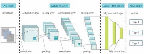
Convolutional neural network (CNN) consists of several basic building blocks, some of which implement basic functions, such as convolution, pooling, full connection and activation. Convolution neural network obtains feature map by convolution operation. At each position, the units from different feature map get different types of features. After a buildup layer, the pooled layer will be connected for down sampling operation, and finally the output result of the fully connected layer will be connected. A simple convolutional neural network structure is given in Figure 1 below. In this part, we mainly describe the basic calculation principle of convolutional neural network. The calculation principle of each different building block (layer) will be introduced below.

Figure 1. Structure diagram of convolutional neural network.

Convolution Layer

Convolution layer is the most important part of CNN. It includes a set of filters (also known as convolution kernel), which convolute with a given input to generate feature map. The size of these filters is (h × w × n), where h is the height, w is width of these filters, and n is the number of channels for a given input image (Uchida, Tanaka, and Okutomi 2018). Convolutional neural network is most commonly used in two-dimensional convolution layer, which has two spatial dimensions of height and width. The size of the commonly used filter is 3 × 3, 5 × 5 or 1 × 1. The two-dimensional convolution formula of two signals is defined as formula (1):

(1) $\mathbf{R}\left(\mathbf{m},\mathbf{n}\right)=\mathit{g}\left(\mathit{m},\mathit{n}\right)\mathbf{\ast }\mathit{f}\left(\mathit{m},\mathit{n}\right)=\sum _{\mathit{i}=-\mathit{n}}^{\mathit{i}=\mathit{n}}\sum _{\mathit{j}=-\mathit{n}}^{\mathit{j}=\mathit{n}}\mathit{f}\left(\mathit{i},\mathit{j}\right),\mathit{g}\left(\mathit{m}-\mathit{i},\mathit{n}-\mathit{i}\right)$(1)

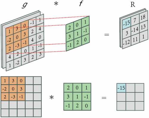
The symbol $\ast$ in the formula represents convolution of two functions; $g\left(m,n\right)$ is the input image, $f\left(m,n\right)$ is the filter, $\mathbf{R}\left(\mathbf{m},\mathbf{n}\right)$ is the result of convolution calculation. We will use a specific example to explain the calculation process. As shown in Figure 2, the input is a two-dimensional array with length and width of 5. Let us record the shape of the array as (5,5). The height and width of convolution kernel array are 3, which is also called filter in calculation. The height and width of convolution kernel determine the shape of convolution kernel window, that is (3,3). The convolution kernel slides on the whole image to generate the output feature map, in which the step size is a super parameter. In this example, the step size is 1. The visualization of the calculation process is shown as:

Figure 2. An example of convolution computation, the step size is 1. The upper part is the convolution operation of multiple pictures, and the lower part is the visualization of one step in the convolution calculation.

Pooling Layer

In real images, the features we are looking for will not always be fixed in the same position: even if the same object is continuously photographed, there will be pixel position offset. This will lead to the same edge corresponding to the output may appear in different positions in the convolution output, and then lead to errors and information loss, causing inconvenience to subsequent recognition. Pooling layer (PL) can alleviate and improve the transition sensitivity of convolution layer to feature location (Scherer, Müller, and Behnke 2010).

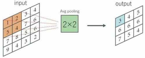
The pooling layer operates the blocks of the input feature map and combines their features to activate. Similar to the convolution layer, you also need to specify the size and stride of the pooling area. According to different calculation methods (maximum or average), they are called maximum stratification layer and average stratification layer. Given the window shape of m × n(in this article, the shape of the matrix in the example is 4 × 4), the maximum value is extracted by maximum pooling, and the average value is extracted by corresponding average pooling. Pooling can effectively down sampling the input feature graph, which can reduce the number of parameters. Two examples of calculation results are shown in Figures 3 and Figure 4:

Figure 3. An example of Max pooling, the step size is 1.

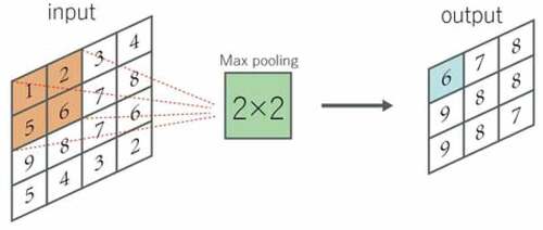
Figure 4. An example of Avg pooling, the step size is 1.

Activation Function

In CNN, the nonlinear activation function is usually used after the weight layer (including convolution layer and fully connected layer), which is also called Activation Layer (AL). The activation function will compress the input value into a small range (such as [0,1] or [- 1,1]), which is convenient for training at the next level. It is important to use the activation function after the weight layer because it allows neural networks to learn nonlinear mapping. In the absence of nonlinearity, the stacked network of weight layers corresponds to a linear mapping between input and output domains. Stacking enough weight layers (or increasing the depth) can theoretically approximate any model function, but such a fitting process will cause the data fitting to be too smooth, even for the data values that do not need to be saved. In fact, the function of activation function is to segment the data categories, to get a better fitting effect. The activation functions used in the model built in this article are listed below.

Sigmoid

Sigmoid is a universally used activation function in neural network, and its expression is shown as formula (2), and the functional relationship image is shown in Figure 5 below:

(2) $f_{sigm}\left(\mathrm{x}\right)=\frac{1}{1+e^{-x}}$(2)

Figure 5. Sigmoid function image.

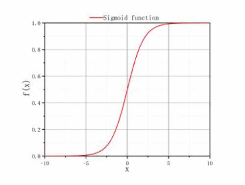
It can convert a real number into a range of (0,1) and is often used for binary classification (Campo et al. 2013). It works better when feature differences are complex or not particularly large, Sigmoid function has the advantages of smoothness and easy derivation. The activation function is applied as the output layer of the deep convolution neural network built in this paper.

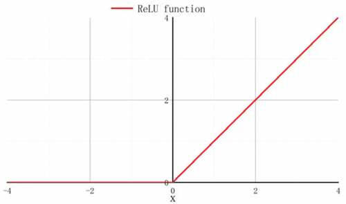
ReLU

ReLU, as an activation function, has special practical significance because of its fast calculation speed (Yarotsky 2017). If the input is negative, the output value activated by the ReLU function is 0; but if the input is positive, the input value will not be changed. ReLU is defined as formula (3), the function image is shown in Figure 6.

(3) $f_{relu}\left(x\right)=\left\{\begin{array}{c}0,x<0\\ x,x\ge 0\end{array}\right.$(3)

Figure 6. ReLU function image.

Fully Connected Layer

In a typical CNN, the full connection layer is placed at the end of the architecture, behind the convolution and pool layers. The fully connected layer corresponds essentially to the convolution layer of a filter of (1 × 1) size, where each cell is densely connected to all the cells of the previous layer (Wu and Zhou 2016).

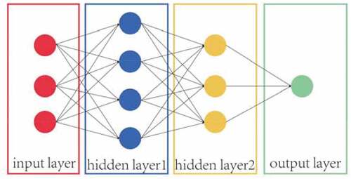
Fully connected layers (FCL) play the role of “Classifier” in the whole convolutional neural network, which maps the learned “distributed feature representation” to the sample label space. The whole fully connected layer is composed of many neurons, also known as perceptron. Perceptron can receive multiple inputs and produce a single output. Figure 7 shows the perceptron and Figure 8 shows a simple fully connected layer. As shown in Figure 7, $x_1$, $x_2$,$x_3$ are the input signal, $y$ is the output signal of the perceptron. Each input signal has a coefficient associated with it, which is also called weight, and the weight reflects the importance of each input to the output. The output of neurons, 0 or 1, is less than or greater than a certain threshold by weighted sum ${\sum }^{w_i}{x}_i$. Many perceptron’s like this stack together to form a fully connected layer. At the end of all convolution pooling processes, the output signature map is flattened and connected to these layers Alqahtani, et al., 2021).

Figure 7. Neuron (Perceptron).

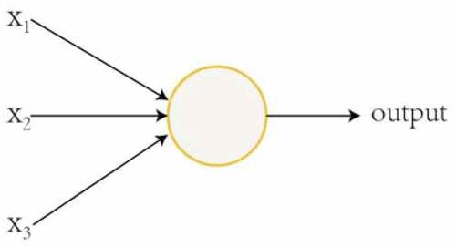
Figure 8. A simple example of fully connected network.

CNN Learning: Loss Function and Small Batch Gradient Descent

Binary Cross-entropy

Loss function is an index to measure the “deterioration degree” of convolutional neural network performance, that is, to what extent the current model does not match the monitoring data, and to what extent it is inconsistent. By minimizing the loss value, the model converges, and the error of model prediction is reduced. Therefore, different loss functions have great influence on the model. The following describes the loss function used in this paper.

Binary cross-entropy is a kind of cross-entropy, when there are only two output results, it is often used to calculate the loss. The expression of binary cross-entropy is given by formula (4), where $y$ is the label(positive value returns 1, negative value returns 0), is the predicted probability of the point being positive for all $n$ points.

(4) $f_p\left(q\right)=-\frac{1}{n}\sum _{i=1}^n{y}_i\cdot lnp\left(y_i\right)+\left(1-y_i\right)\cdot ln\left(1-p\left(y_i\right)\right)$(4)

Mini-Batch Gradient Descent

CNN’s learning process is precisely through adjusting the network parameters to make the input space and output space match correctly. In other words, the learning process is to minimize the loss by optimizing its parameters. The most intuitive but simple way to solve this problem is to make the loss function gradually reduce to the minimum by repeatedly updating the parameters. The gradient-based method is to find out the position with the largest change rate (that is, the steepest descent direction), and update and optimize the parameters along this direction. The learning rate is the super parameter that guides how to adjust the weight of the network through the gradient of the loss function, that is, the size of the parameter update. Each iteration in the training process of the training set is called the training period. At time t, the parameter updating equation of each training iteration is given by formula(5) and formula(6):

(5) ${\theta }_t={\theta }_{t-1}-\eta {\delta }_t$(5)

(6) ${\delta }_t={\mathrm{\nabla }}_{\theta }\mathrm{\Gamma }\left({\theta }_t\right)$(6)

In the above formula: $\mathrm{\Gamma }\left(\cdot \right)$ is the function represented by the neural network function with parameter $\theta$, $\mathrm{\nabla }$ is the gradient, and $\eta$ is the learning rate.

Small batch gradient descent is a compromise between batch gradient descent and random gradient descent. It divides the training set into several small batches, and each small batch is composed of relatively few training samples, which improves the convergence efficiency and stability. Then the gradient of each small batch is calculated, and the parameters are updated. Usually, training samples are randomly combined to improve the homogeneity of training set.

Training Model

In this paper, based on four deep convolution neural network structures: VGG19 (Carvalho et al. 2017), InceptionV3 (Zhao et al. 2020), ResNet50 (Wu, Shen, and Hengel 2019) and Xception (Chollet F .2017). Their input structure is changed to 256 * 256 * 3, and their classifiers are reconstructed adaptively.

After the convolution layer structure output the results, a global pooling layer is connected for average pooling to facilitate the connection of the fully connection layer, and then three fully connection layers are connected with the parameter sizes (number of neurons) of 512, 256, and 64, respectively.

In addition, dropout layers of the same size are added after each fully connection layer. During training, each time the data is transmitted, the dropout layer will randomly select and delete the neuron signals, and the deletion ratio of the model is set to 20% to suppress the over fitting of the model.

The programming language used in the experiment is Python, and the network models are built based on the framework of TensorFlow. CPU information: Intel(R) Core (TM) i9-10,900 K CPU @3.70 GHz 3.70 GHz, RAM:64GB. The optimization function used in the experiment is Adam optimizer. Adam optimizer is an effective random optimization method. It only needs a first-order gradient and only needs a small memory. The method calculates the adaptive learning rate of different parameters through the estimation of the first and second gradients.

Different learning rate often led to different performance of the models. Too large learning rate will make the gradient drop too fast, resulting in the situation that the loss function keeps jumping around the extreme point but cannot find the extreme point; Too small learning rate often leads to the slow decline of gradient, and even the stagnation of loss function. Therefore, during the experiment, the learning rate can be set according to the rate at which the loss value decreases, after the comprehensive experiment, the learning rate is set as 1 × 10⁻⁴.

Results and Discussion

Data Preparation

The dataset SDNET2018 used in this paper is from Mark Maguire, a researcher of Utah State University in the United States (Dorafshan, Thomas, and Maguire 2018). It is a dataset for training, verification and benchmark of concrete crack detection algorithm based on artificial intelligence. SDNET2018 contains images of cracked and uncracked concrete decks. The data set includes cracks as narrow as 0.06 mm and as wide as 25 mm. These images are color images, including images of various obstacles. Mark the images as type C (cracked) and type U (uncracked) according to whether there are cracks in the images. The pictures of cracked and uncracked concrete bridge decks are shown in Figures 9 and Figure 10 below:

Figure 9. All above are cracked images. From top to bottom: unclear and hard to detect cracks; small cracks; obvious and clear cracks.

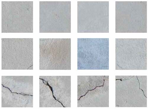
Figure 10. All above are uncracked images. The upper part are smooth uncracked images, the lower part are rough uncracked images.

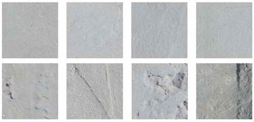
Image Enhancement

As the photos in the data set are all real photos, there are few photos of concrete bridge deck with cracks (only 2,025 in total, accounting for about 15% of the total). In addition, the background of each image is very similar, occupying a large area. Based on the above reasons, too little learning information may lead to the convolutional neural network cannot fully learn features and reach saturation, so the image enhancement method is used to increase the learning information.

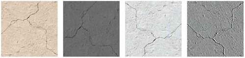
In this paper, three methods are used to enhance the image of the original data set. The first is to flip the image randomly (including up and down and left and right); The second is to change the color randomly, from brightness, contrast, saturation, and hue to change the color of the image; Finally, the gray value and hue conversion are adjusted randomly. In the actual processing, the image is randomly superimposed by three effects. The following two groups of images show the effect after image enhancement. Figure 11 is an original cracking image, and Figure 12 shows four images after four times of image enhancement;

Figure 11. An image of the original crack in the dataset.

Figure 12. Four images are obtained by image enhancing.

Data Division

The dataset is divided into training data and validation data, accounting for approximately 4:1. A small batch random gradient descent method is used for training, and validation datasets are tested at the same time during each small batch training process. Based on the previous step (image enhancement), the total number of surface images of concrete was expanded to 98,512, all color images were resized to 256 × 256, and the information of three channels (R, B, and G) was preserved. The dataset is divided into 78,705 training images and 19,807 test images to make the deep convolution neural network fully trained. Table 1 is the number of images before image enhanced, Table 2 shows the number of different types of images after image enhancement.

Table 1. Number of images before augmentation

Class type	Train folder	Test folder	Total(class)
Un-cracked	1620	405	2025
Cracked	9276	2319	11,595
Total(folder)	10,896	2724	13,620

Table 2. Number of images after enhancement

Class type	Train folder	Test folder	Total(class)
Un-cracked	37,932	9676	47,608
Cracked	40,773	10,131	50,904
Total(folder)	78,705	19,807	98,512

Experimental Result

To explore the advantages of deep convolutional neural network over ordinary convolutional neural network, a shallow convolution neural network, and fully connected neural network are constructed. The former has 10 layers, of which seven layers are convolutional layer and three layers are fully connected layer, it also has three pooling layers and three Dropout layers. Another fully connected neural network (FCNN) structure is also constructed as a ten-layer structure, it also has three Dropout layers.

Table 3 shows the number of layers of the network structure and the training parameters they have.

Table

Model	Total layers	Trainable params	Total params
VGG19	29	20,189,761	20,190,785
InceptionV3	318	22,330,017	22,368,545
ResNet50	182	24,096,257	24,153,473
Xception	139	21,368,617	21,427,241
CNN	16	500,897	501,153
FCNN	13	2,111,425	2,111,489

To get stable results and make the results effective. The same number of training sets and test sets are used for the models constructed in this paper, and the loss function and activation function of each model are compared. The optimizer and learning rate are unified. The intermediate results in the model are normalized in batches, and the dropout layer is used to suppress the over fitting after the full connection layer. The most stable results were obtained after 10 cross validations of each model. Finally, we adjusted the training process to a total of 100 epochs, The optimizer Adam is used and set the learning rate to $1\times {10}^{-4}$, binary cross-entropy is used as a loss function. We use loss value, RMSE value and accuracy as the evaluation criteria for model performance. The lower the loss value and RMSE value, the higher the accuracy rate, the better the model performance, on the contrary, the worse the model performance. Table 4 shows loss values, RMSE values, and correctness rates for all models, Figures 13, Figure 14 and Figure 15 shows the change trend of loss, RMSE, and accuracy during all model training processes, respectively.

Table 4. Loss, RMSE and accuracy of cross-validation results for each prediction model

Model	Loss	RMSE	Accuracy
VGG19	0.1790	0.2700	0.9297
InceptionV3	0.0958	0.2081	0.9639
ResNet50	0.1310	0.2616	0.9479
Xception	0.1297	0.2213	0.9520
CNN	0.4251	0.4283	0.7955
FCNN	0.6375	0.4776	0.6394

Figure 13. Change trend of loss.

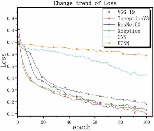
Figure 14. Change trend of RMSE.

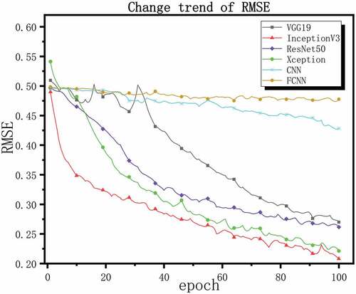
Figure 15. Change trend of accuracy.

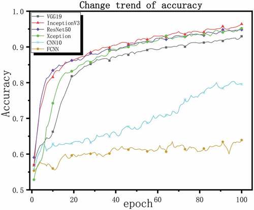
From the above results, it can be seen that the deep convolutional neural network structure shows better performance than the shallow structure during training. However, even if a large enough training data set is used, it is difficult for shallow networks to extract the feature information of complex images. We can see that their loss value decreases slowly or even hard, and the accuracy is also very low. The four deep performances seem to be equal during training. To further explore their performance more accurately, we save the trained network and reverify them with new evaluation indexes.

Before that, we need to introduce some concepts TP, TN, FP, and FN. TP (True Positive): Positive samples predicted as positive by the model; it can be called the correct rate of judging to be true. TN (True Negative): Negative samples predicted as negative by the model; it can be called the correct rate of judging as false. FP (False Positive): Negative samples predicted as positive by the model; it can be called false-positive rate. FN (False Negative): Positive samples predicted as negative by the model; it can be called the false-positive rate.

The new evaluation indexes are accuracy rate, F1 index and recall rate, and the calculation formula are given below:

(7) $precision:P=\frac{TP}{TP+FP}$(7)

(8) $Recall:R=\frac{TP}{TP+FN}$(8)

(9) $F_1\sim score:F_1=\frac{2}{\frac{1}{P}+\frac{1}{R}}$(9)

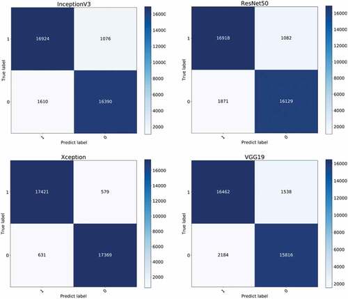
We randomly selected 18,000 cracked images and 18,000 uncracked images from the expanded dataset, and made the same marks as in the experiment, that is, cracked images are marked as positive samples and uncracked images are marked as negative samples. Then the four networks are further verified at the same time (the shallow network structure with poor performance is no longer verified). The confusion matrix results are shown in Figure 16, The new indexes are calculated as shown in Table 5.

Table 5. Results of precision, recall and F₁-score

Model	P	R	F1
Xception	0.9650	0.9678	0.9664
InceptionV3	0.9131	0.9402	0.9264
ResNet50	0.9004	0.9399	0.9197
VGG19	0.8829	0.9146	0.8985

Figure 16. Confusion matrix results of four models.

Based on all the above results, it can be seen that the deep network structure shows better performance during training, the loss function and RMSE decline rapidly, and can reach a very low value, and the accuracy of verification is very high. After further experiments, it is found that although the performance of the four models seems to be similar during training, they still show different performances after reverification.

According to the new evaluation index, we draw the following conclusions about the performance of the model: Xception>InceptionV3> ResNet50> VGG19. As can be seen from Table 5, all indicators of Xception are very good, which are higher than 96%. In contrast, although the recall rates of InceptionV3 and ResNet50 are not low, the accuracy rate and F1 index are quite different from Xception, and the performance of VGG19 is even worse. We can find the reason from Figure 16, InceptionV3 and ResNet50 can also effectively identify the cracked image, but they will mistakenly regard some uncracked images as cracked images. Xception can recognize two types of images, and the accuracy is higher than them, so its indicators are very good. Finally, we have obtained a crack identification model with excellent performance in all aspects through experiments.

To verify the universality of the model (Xception), we also conducted cross dataset research, we found images on the Internet. Dataset-1: 40,000 concrete crack images (Zgenel and Sorguc 2018) and Dataset-2: 6069 bridge crack images (Xu et al. 2019). Model is used to identify these images. All the data in the dataset are directly used as the verification data. The verification method is the same as the above. The results of the confusion matrix are as Figure 17 and Table 6.

Table 6. Precision, recall and F₁-score of cross-datasets research

Dataset	P	R	F1
Dataset-1	0.9823	0.9918	0.9870
Dataset-2	0.9904	0.9869	0.9886

Figure 17. Confusion matrix results of cross-datasets research.

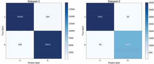
It can be seen that in the experiments across-datasets, the model shows better performance. After recognizing the images of two different datasets, the recognition precision is as high as 98.23% and 99.04%. This proves the strong adaptability and applicability of the model, and also shows that the model is also practical in real life.

Conclusions

Based on the basic framework of four deep convolution neural networks, their classifiers are reconstructed, and a concrete crack recognition model is established. In order to solve the problem of insufficient training data and make the constructed model fully trained, the method of image enhancement is adopted. Through the superposition of various methods such as random flipping, changing illumination and changing color saturation, the situation of shooting from different angles and different weather environments in real life is simulated. Different from the shallow structure, the four deep models show good performance in the training process. It can be seen from the experimental data that in the face of complex data, the depth model can better extract the feature information in the image than the shallow model.

To accurately measure the performance of the four models, they were tested with new indicators, and the results of additional experiments showed that although they performed well in the training process, there were differences. Obviously, Xception has better performance in further research experiments. It can be seen from Table 5 that its precision, recall, and F₁-score exceed 96.5%. From the result diagram of confusion matrix, it can be seen that Xception has high recognition accuracy for positive and negative samples, while other models will regard many negative samples (uncrack images) as positive samples (crack images) although they perform well in the recognition of positive samples. In terms of universality, the model can accurately identify cross data sets, and the accuracy of identifying new concrete crack images and bridge crack images are 98.23% and 99.04%, respectively.

In general, the research of this paper shows that when facing images with complex information and difficult to identify, deep convolution neural network has advantages when fully trained by expanding data set and adjusting network structure combination parameters. The fully trained model also has excellent recognition ability on different data sets (facing the complex situation of different environments in life). This provides a feasible theoretical basis for crack identification of concrete structure. However, in real life, the concrete crack mode may be more complex and changeable than that in this study. The length, width and direction of cracks have an important influence on the failure of building structures. Therefore, it is necessary to accurately extract the important features of complex cracks. In the future work, various complex crack images will be collected directly, and the deep learning method will be used to detect the cracks on the image, so as to accurately determine the location and specific shape of the cracks.

Project And Fund

1. No. 5802, Talents of Guizhou science and technology cooperation platform (2019).

2. No. 2886, Support of Guizhou science and technology cooperation (2019).

Disclosure Statement

No potential conflict of interest was reported by the author(s).

Correction Statement

This article has been republished with minor changes. These changes do not impact the academic content of the article.

Additional information

Funding

This work was supported by the Support of Guizhou science and technology cooperation (2019). [No. 2886]; Talents of Guizhou science and technology cooperation platform (2019). [No. 5802].

References

- Ahmadkhah, S. M., R. P. R. Hasanzadeh, and M. Papaelias. 2019. Arbitrary crack depth profiling through ACFM data using Type-2 fuzzy logic and PSO algorithm. Ieee Transactions on Magnetics 55 (2):1–1248. doi:10.1109/tmag.2018.2884828.
- Ahmed, M. O., R. Khalef, G. G. Ali, and I. H. El-adaway. 2021. Evaluating deterioration of tunnels using computational machine learning algorithms. Journal of Construction Engineering and Management 147 (10):04021125. doi:10.1061/(asce)co.1943-7862.0002162.
- Alqahtani, H, S Bharadwaj, and A Ray. 2021. Classification of fatigue crack damage in polycrystalline alloy structures using convolutional neural networks. Engineering Failure Analysis. 119 (104908). doi:10.1016/j.engfailanal.2020.104908.
- Annamdas V. G. M., Bhalla S., and Soh C. K. 2017. Applications of structural health monitoring technology in Asia[J]. Structural Health Monitoring 16 (3): 324–346. doi:10.1177/1475921716653278
- Campo, I. D., R. Finker, J. Echanobe, and K. J. E. L. Basterretxea. 2013. Controlled accuracy approximation of sigmoid function for efficient FPGA-based implementation of artificial neurons. Cortex; a Journal Devoted to the Study of the Nervous System and Behavior 49 (6):1598–600. doi:10.1016/j.cortex.2012.07.011.
- Carvalho, T., Rezende, E., Alves M., et al. Exposing Computer Generated Images by Eye’s Region Classification via Transfer Learning of VGG19 CNN[C]// 16th IEEE International Conference On Machine Learning And Applications. IEEE, 2017. DOI: 10.1109/ICMLA.2017.00-47.
- Chen, C., and B. Zhao. 2017. A modified Brownian force for ultrafine particle penetration through building crack modeling. Atmospheric Environment 170:143–48. doi:10.1016/j.atmosenv.2017.09.035.
- Chollet, F., “Xception: deep learning with depthwise separable convolutions,” 2017 IEEE Conference on Computer Vision and Pattern Recognition (CVPR) Honolulu, HI, USA, 2017, pp. 1800–07. doi: 10.1109/CVPR.2017.195.
- Cui, X., Q. Wang, J. Dai, Y. Xue, and Y. Duan. 2021. Intelligent crack detection based on attention mechanism in convolution neural network. Advances in Structural Engineering 24 (9):1859–68. doi:10.1177/1369433220986638.
- Dorafshan, S., R. J. Thomas, and M. Maguire. 2018. SDNET2018: An annotated image dataset for non-contact concrete crack detection using deep convolutional neural networks[J]. Data in Brief 21:1664–68. doi:10.1016/j.dib.2018.11.015.
- Feng, C. C., H. Zhang, S. Wang, Y. L. Li, H. R. Wang, and F. Yan. 2019. Structural damage detection using deep convolutional neural network and transfer learning. KSCE Journal of Civil Engineering 23 (10):4493–502. doi:10.1007/s12205-019-0437-z.
- Fu, Y. X., J. Z. Ming, W. Lei, and R. Jian. 2016. Recent highway bridge collapses in China: review and discussion. Journal of Performance of Constructed Facilities. 30 (5):04016030. doi:10.1061/(ASCE)CF.1943-5509.0000884.
- Guo, X., Y. T. Yuan, and Y. Liu. 2021. Crack propagation detection method in the structural fatigue process[J]. Experimental Techniques 45 (2):169–78. doi:10.1007/s40799-020-00425-1.
- Jeyaraj, P. R., and E. R. S. Nadar. 2019. Computer vision for automatic detection and classification of fabric defect employing deep learning algorithm. International Journal of Clothing Science and Technology 31 (4):510–21. doi:10.1108/ijcst-11-2018-0135.
- Kim, B., and S. Cho. 2018. Automated vision-based detection of cracks on concrete surfaces using a deep learning technique. Sensors 18 (10):18. doi:10.3390/s18103452.
- Kim, H., E. Ahn, M. Shin, and S. H. Sim. 2019. Crack and noncrack classification from concrete surface images using machine learning. Structural Health Monitoring-an International Journal 18 (3):725–38. doi:10.1177/1475921718768747.
- Kong, X. 2019. Li JJAiC. Non-contact Fatigue Crack Detection in Civil Infrastructure through Image Overlapping and Crack Breathing Sensing 99 (MAR.):125–39. doi:10.1016/j.autcon.2018.12.011.
- Nhat-Duc, H., N. Quoc-Lam, and B. Dieu Tien. 2018. Image processing-based classification of asphalt pavement cracks using support vector machine optimized by artificial bee colony. J Comput Civil Eng 32 (5). doi: 10.1061/(asce)cp.1943-5487.0000781.
- Ozcelik, M. 2018. Back analysis of ground vibrations which cause cracks in buildings in residential areas Karakuyu (Dinar, Afyonkarahisar, Turkey). Natural Hazards 92 (1):497–509. doi:10.1007/s11069-018-3215-1.
- Scherer, D., Müller A., and Behnke S. Evaluation of pooling operations in convolutional architectures for object recognition[C]// International conference on artificial neural networks. Springer, Berlin, Heidelberg, 2010: 92–101. doi: 10.1007/978-3-642-15825-4_10.
- Sm, A., A. Qr, and B. Mua. 2021. Cs BJMS, Processing S. Causal Dilated Convolutional Neural Networks for Automatic Inspection of Ultrasonic Signals in Non-destructive Evaluation and Structural Health Monitoring 157. doi:10.1016/j.ymssp.2021.107748.
- Sokolov, S. S., N. B. Glebov, E. N. Antonova, and A. P. Nyrkov, editors. The safety assessment of critical infrastructure control system. 2018 IEEE International Conference” Quality Management, Transport and Information Security, Information Technologies”(IT&QM&IS), St. Petersburg, Russia; 2018: IEEE. 10.1109/ITMQIS.2018.8524948.
- Spencer, J. B. F., V. Hoskere, and Y. Narazaki. 2019. Advances in computer vision-based civil infrastructure inspection and monitoring[J]. Engineering 5 (2):199–222. doi:10.1016/j.eng.2018.11.030.
- Sun, J. P., J. J. Zhang, W. F. Huang, L. Zhu, Y. T. Liu, and J. W. Yang. 2020. Investigation and finite element simulation analysis on collapse accident of Heyuan Dongjiang Bridge. Engineering Failure Analysis 115:10. doi:10.1016/j.engfailanal.2020.104655.
- Uchida, K., M. Tanaka, and M. Okutomi. 2018. Coupled convolution layer for convolutional neural network. Neural Networks 105:197–205. doi:10.1016/j.neunet.2018.05.002.
- Wu, J., “Compression of fully-connected layer in neural network by Kronecker product,” 2016 Eighth International Conference on Advanced Computational Intelligence (ICACI), Chiang Mai, Thailand, 2016, pp. 173–79, doi: 10.1109/ICACI.2016.7449822.
- Wu, Z., C. Shen, and A. J. P. R. Hengel. 2019. Wider or deeper: revisiting the ResNet model for visual recognition. Pattern Recognition. 90:119-133. doi:10.1016/j.patcog.2019.01.006.
- X.Q, and S. S. Zhu. 2015. Engineering LJAiS. Structural Health Monitoring Based on Vehicle-Bridge Interaction: Accomplishments and Challenges 18 (12):1999–2015. doi:10.1260/1369-4332.18.12.1999.
- Xu, H. Y., X. Su, Y. Wang, H. Y. Cai, K. R. Cui, and X. D. Chen. 2019. Automatic bridge crack detection using a convolutional neural network[J]. Applied Sciences-Basel 9:14. doi:10.3390/app9142867.
- Yang, Q., W. Shi, J. Chen, and W. Lin. 2020. Deep convolution neural network-based transfer learning method for civil infrastructure crack detection. Automation in Construction 116. doi:10.1016/j.autcon.2020.103199.
- Yarotsky, D. 2017. Error bounds for approximations with deep ReLU networks. Neural Networks 94:103–14. doi:10.1016/j.neunet.2017.07.002.
- Ye, X W, T Jin, and C B Yun. 2019. A review on deep learning-based structural health monitoring of civil infrastructures. Smart Struct Syst 24 (5):567–586. doi:10.12989/sss.2019.24.5.567.
- Ye, X W, T Jin, and P Y Chen. 2019. Structural crack detection using deep learning-based fully convolutional networks. Advances in Structural Engineering 22 (16):3412–3419. doi:10.1177/1369433219836292.
- Yu, Y., C. Wang, X. Gu, and J. Li. 2019. A novel deep learning-based method for damage identification of smart building structures. Structural Health Monitoring 18 (1):143–63. doi:10.1177/1475921718804132.
- Yu, Y., M. Rashidi, B. Samali, A. M. Yousefi, and W. Wang. 2021. Multi-image-feature-based hierarchical concrete crack identification framework using optimized SVM multi-classifiers and D–S fusion algorithm for bridge structures. Remote Sensing 13 (2):240. doi:10.3390/rs13020240.
- Zgenel, F., and A. G. Sorgu, editors. Performance comparison of pretrained convolutional neural networks on crack detection in buildings. 35th International Symposium on Automation and Robotics in Construction (ISARC 2018) Berlin, Germany; 2018.doi: 10.22260/ISARC2018/0094.
- Zhao, Y., K. Xie, Z. Zou, and J.-B. He. 2020. Intelligent recognition of fatigue and sleepiness based on inceptionV3-LSTM via multi-feature fusion. IEEE Access 8:144205–17. doi:10.1109/ACCESS.2020.3014508.