Prediction in Traffic Accident Duration Based on Heterogeneous Ensemble Learning

ABSTRACT

Based on millions of traffic accident data in the United States, we build an accident duration prediction model based on heterogeneous ensemble learning to study the problem of accident duration prediction in the initial stage of the accident. First, we focus on the earlier stage of the accident development, and select some effective information from five aspects of traffic, location, weather, points of interest and time attribute. Then, we improve data quality by means of data cleaning, outlier processing and missing value processing. In addition, we encode category features for high-frequency category variables and extract deeper information from the limited initial information through feature extraction. A pre-processing scheme of accident duration data is established. Finally, from the perspective of model, sample and parameter diversity, we use XGBoost, LightGBM, CatBoost, stacking and elastic network to build a heterogeneous ensemble learning model to predict the accident duration. The results show that the model not only has good prediction accuracy but can synthesize multiple models to give a comprehensive degree of importance of influencing factors, and the feature importance of the model shows that the time, location, weather and relevant historical statistics of the accident are important to the accident duration.

Introduction

With a rapid development of global urbanization, the traffic congestion has become an increasingly serious problem. Traffic congestion can have significant adverse effects on the economy, society and the environment. Any traffic incidents that reduce safety and slow down traffic speed, such as accidents, leakage of hazardous materials, are one of the main factors contributing to traffic congestion (Mfinanga and Fungo 2013). Traffic congestion is usually divided into recurrent and non-recurrent traffic congestion (Dowling, Skabardonis, and Carroll et al. 2004; Hojati, Ferreira, and Washington et al. 2014). Recurrent traffic congestion occurs when the road is beyond its capacity, while non-recurrent congestion is a temporary reduction in normal capacity caused by incidents, maintenance work or construction activities, and special events where peak demand is higher than normal (Aldeek and Emam 2006). In order to facilitate the managers to better manage traffic incidents, further improve traffic safety, reduce the loss caused by traffic accident congestion, and ensure the travel safety of travelers and the quality of travel services, thereby reducing the traffic operation burden and alleviating traffic congestion, the question is of great significance to the study of the duration of the accident.

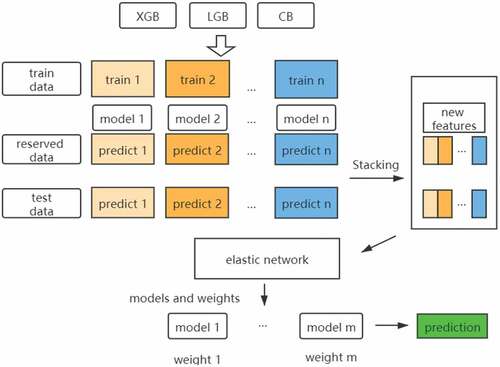
Figure 1. Heterogeneous integration stacking process.

Incident duration refers to the time elapsed from the occurrence of the incident to the removal of all evidence of the incident from the scene (Valenti, Lelli, and Cucina 2010). Haule, Sando, and Lentz et al. (2019) gave a different definition of incident duration, which is divided into four stages: detection, response, clearance, and recovery, of which some stages ignore incident detection time or recovery time. In recent years, much attention has been devoted to predicting the duration of traffic incidents. The methods for the duration of incidents mainly include risk-based models (Li, Pereira, and Ben-Akiva 2015; Nam and Mannering 2000; Hojati, Ferreira, and Washington et al. 2013), regression model (Khattak, Liu, and Wali et al. 2016; Wang, Chen, and Zheng 2013), fuzzy model (Dimitriou and Vlahogianni 2015), Bayesian network (Cong, Chen, and Lin et al. 2018; Demiroluk and Ozbay 2014; Ozbay and Noyan 2006) and machine learning model (Hamad, Khalil, and Alozi 2020; Ma, Ding, and Luan et al. 2017; Tang, Zheng, and Han et al. 2020).

Compared with methods, such as risk-based models, regression models and fuzzy models, machine learning methods have higher accuracy in incident duration prediction, a wider range of applications and significant advantages. Hamad, Alruzouq, and Zeiada et al. (2020) used a data set containing more than 50 variables from more than 140,000 incidents records in the Houston metropolitan area of Texas, who established random forest (RF) models to predict incidents with duration ranging from 1 to 1440 minutes and 5 to 120 minutes, and compared with artificial neural networks (ANN), the results showed that the mean absolute error (MAE) of the random forest model was 14.979 minutes and 36.652 minutes for the two events, respectively. Ma, Ding, and Luan et al. (2017) used 1366 incidents data and historical weather data from Washington in 2012 to divide incident clearance time into two categories with 15 minutes as a threshold, established gradient boosting decision trees (GBDT) to predict incident clearance time. By comparing the different parameters of the model, the mean absolute percentage error (MAPE) of the long-duration and short-duration optimal models are 33.13% and 16.44%, respectively. Compared with BP neural network, support vector machine (SVM) and RF, GBDT is better than the other three models in predicting the clearance time of two categories of events. Tang, Zheng, and Han et al. (2020) used XGBoost algorithm to study 2565 incidents clearance time in a high incident-occurrence area of Washington in 2012. They used the K-means to cluster the data into 2 categories, and then used XGBoost to predict the incident removal time of the two clusters. Their results show that the performance of XGBoost in the two clusters is better than SVM regression, RF and Adaboost, MAPE is 34.8% and 22.1%, respectively, and the important factors that affect the incident clearance time are the annual average daily traffic, event type, response time and lane closure type.

In addition, there are researchers who specialize in comparative investigation on multiple methods. Hamad, Khalil, and Alozi (2020) compared the effects of regression decision tree, SVM, ensemble tree, Gaussian process regression (GPR) and ANN models in predicting the duration of traffic incidents based on 110000 short-time event records containing more than 50 variables (duration ranging from 5 minutes to 120 minutes), In terms of MAE, SVM is better than other models. However, in terms of root mean square error (RMSE), SVM is the worst and GPR is the best. In terms of training time, regression decision tree requires the shortest training time, while SVM and GPR require a longer training time. By calculating the congestion delay index, Lin and Li (2020) studied the duration of four different traffic conditions after traffic accidents based on crowdsourcing data. A total of 13,338 traffic accident records in Beijing in 2017 were used to verify and compare the effects of RF, SVM and neural network (NN). The results show that the NN model performs better than the other two models in most cases.

In view of the shortcomings of most previous studies, such as small data volume, limited application region, and lack of upstream and downstream information of the event, Moosavi, Samavatian, and Parthasarathy et al. (2019b) used points of interest in accident prediction for the first time. In addition, large heterogeneous data of about 2.25 million traffic events occurred in the United States from February 2016 to March 2019 were collected, expanded, sorted, and created. Based on the comprehensive data collection, the model is divided into accident and non-accident classification problems, and a deep-neural-network-based accident prediction model named deep accident prediction (DAP) is established for real-time aident prediction, and compared with the logistic regression (LR), gradient boosting classifier (GBC) and deep neural network (DNN) models, the results show that the performance of the model is superior.

From the perspective of research objects, previous studies on accident duration were mostly dependent on the modeling of a certain highway, certain city, certain province or state, which had the disadvantages of small sample size and limited application region. On the other hand, from the selection of influencing factors related to the accident duration, part of the prediction of the accident duration includes some information that can only be obtained after the accident, but in fact, the information available at the time of the accident is very limited, so it is not meaningful to use too many factors to make prediction. Moreover, earlier reasonable prediction of the accident duration will be conducive to the follow-up rescue work of relevant departments and provide better travel service quality for driver. From the perspective of research methods, the research methods of event duration in recent years mainly include risk-based model, regression model, fuzzy model, machine learning model and so on. With the development of the era of big data, the application of machine learning is more and more widely, tree-based models have high accuracy and interpretability and can also be applied to large data sets. In addition, most of the researches only build models after simple data cleaning on the basic data and fail to explore the deeper relationships between variables through feature engineering, and most of the researches only use one model to give the final result, and fail to combine multiple models. The advantage of combining multiple models can make the final result more valuable for reference.

Therefore, in the present study, we use ensemble learning to investigate the problem of accident duration prediction in the initial stage of accident, our contributions in this paper are as follows. (1) This paper is based on an earlier stage of the accident to study the problem of predicting the duration of traffic accidents, and a large data set of traffic accidents with more than one million records is taken as an example to meet the needs of the era of big data and make the results more valuable and general; (2) We process the original data through data cleaning, category feature coding and other means, and extract deeper information from limited initial information through feature construction. A data pre-processing scheme for accident duration is established and data quality is further improved; (3) Considering the accuracy, interpretability and stability of the model comprehensively, we construct a heterogeneous ensemble learning model for accident duration prediction from the perspective of model, sample and parameter diversity. The model can give the comprehensive influence of relevant factors of multiple models on the prediction of accident duration while maintaining good prediction effect.

Data Preprocessing and Feature Engineering

Data Description

In this paper, data are selected from the data set “US Accidents” published by Kaggle (Moosavi, Samavatian, and Parthasarathy et al. 2019a), which is a nationwide data set for accidents in 49 states in the US, spanning from February 2016 to June 2020. Since the original data comes from two APIs. Taking into account the unity of data metrics, the car accident data provided by API MapQuest with the majority of data are selected for research.

The focus of this paper is to consider how to better predict the duration of the accident through some relatively easily available variables when a traffic accident is verified. Therefore, variables that can only be obtained after the accident, such as the description of the accident and the severity of the accident, will be discarded. Through screening, the feature of the traffic attribute, location attribute, weather attribute, points of interest (POI) attribute, and time attribute selected in this paper are shown in Table 1.

Table 1. Original basic characteristics

Attribute	Characteristic variable
Traffic	TMC, Start time, End time, Start lat(latitude), Start lng(longitude)
Location	Street, Side(right/left), City, County, State, Zipcode, Airport code
Weather	Temperature(F), Wind chill(F), Humidity(%), Pressure(in), Visibility(mi), Wind direction, Wind speed(mph), Precipitation(in), Weather condition
POI	Amenity(true or false), Bump, Crossing, Give Way, Junction, No Exit, Railway, Roundabout, Station, Stop, Traffic Calming, Traffic Signal, Turning Loop
Time	Timezone, Sunrise sunset(day or night), Civil twilight, Nautical twilight, Astronomical twilight

Data Preprocessing

Data errors may occur during data recording and transmission, since the End time of a few records is earlier than the Start time, the Start time and the End time of this part of data are swapped, and the accident duration is calculated by the difference between the End time and the Start time. The data set is divided into training set, offline test set and online test set in a ratio of 98:1:1 (Raschka 2015), which the offline test set is used as reserved samples and online test set was used to simulate future data to measure the final model effect. Then, discard the records with the End time of the training set later than the earliest Start time of the test set and finally get a total of 2366002 initial training set data, the time span is from February 8, 2016 to May 14, 2020, and there were 24143 records in the offline test set and online test set, respectively, from May 14, 2020 to June 30, 2020. In the initial training set, the average duration of the accident is 50.50 minutes, the quarter-quantile, median and third-quarter quantile are 29.7 minutes, 44.27 minutes and 59.67 minutes, respectively. The longest accident duration is 336960 minutes and the shortest is 0.27 minutes, both of which are likely outliers.

Outlier Value Preprocessing

Outliers refer to observations that clearly deviate from the rest of the observations. Common outlier detection methods in statistical methods include Z-score method and interquartile range (IQR) method. The Z-score method assumes that the data obeys a normal distribution, while IQR does not depend on a specific distribution and has a wider range of applications. Considering that when IQR is used to detect outliers, some abnormal points cannot be properly processed. Therefore, the reserved samples is used as a reference to delete records with obvious abnormal data in the training set. That is, the minimum and maximum values of the reserved samples are used as the boundary, and the data that exceeds this boundary $a$ and $b$ is screened out in the training set, then delete the records that belong to data smaller than $Q_1^a-1.5(Q_3^a-Q_1^a)$ or larger than $Q_3^b+1.5(Q_3^b-Q_1^b)$ among these data. The variables with obvious outliers are preliminarily determined by the distribution diagrams of the training set and the reserved dataset, including Temperature, Visibility, and Wind Speed. After the above steps, delete records with obvious abnormal values. Considering the time span of the reserved samples, the temperature variable in the training set only deals with abnormal data greater than $Q_3^b+1.5(Q_3^b-Q_1^b)$. In addition, we observed outliers in the duration of accidents in the training set, so 12 records with duration less than or equal to 2 minutes and duration greater than 100,000 minutes were deleted.

Missing Value Processing

Data loss may also be caused in the process of data recording and transmission, so data loss is inevitable. Similarly, there is missing data in this data set, which is shown in Table 2.

Table 2. Missing data

Feature	Missing rate(%)	Feature	Missing rate(%)
City	0.0021	Wind direction	1.4068
Zipcode	0.0128	Wind speed(mph)	14.0116
Timezone	0.0854	Precipitation(in)	62.9072
Airport code	0.1708	Weather condition	1.9682
Temperature(F)	1.6342	Sunrise sunset	0.0022
Wind chill(F)	58.7179	Civil twilight	0.0022
Humidity(%)	1.7422	Nautical twilight	0.0022
Pressure(in)	1.4040	Astronomical twilight	0.0022
Visibility(mi)	1.9697

The missing rate of Wind chill and Precipitation is higher than 50%. If they are filled in, large errors will be introduced, so these two variables are discarded. According to the missing variables, we divide the training set into a non-missing training set denoted by $Trn$, missing training set denoted by $Tr{n}_2$, and non-missing offline test set denoted by $Te{s}_1$ is used for evaluation. In consideration of data volume and prediction effect, $Trn$ is divided into training set $Tr{n}_1$ and validation set $Va{l}_1$ at a ratio of 3:1, and the variables are processed in different situations.

(1) City, Zipcode, Timezone, Airport code

City, Zipcode, Timezone and Airport code are closely related to location. They can be predicted well by the latitude and longitude, so the longitude and latitude of the accident are selected as input variables. We choose k-nearest neighbor (KNN) (Cover and Hart 1967) to fill it and use the grid search method to select a reasonable value of $K$, that is, according to the performance on $Te{s}_1$, the approximate value range is first determined by a large step size, and then the optimal value of $K$ is determined within this range.

In addition, in the variable of Zipcode, some codes are specific to 9 digits, while some only have 5 digits, such as “43068–3402” and “45176”, therefore, in order to better fill it, the fuzzy 5-bit code is taken as the filling target. For variables, such as City, 5-digit Zipcode, Timezone and Airport code, when  $K=1$, KNN has the highest prediction accuracy, which are 97.93%, 96.94%, 99.99% and 99.26%, respectively. Therefore, the case of  $K=1$ is selected to make a predictive filling of the truly missing data.

(2) Wind direction, Weather conditions, Side

Since the factors related to Wind direction and Weather conditions are too complex, the prediction of these two variables by available variables cannot achieve ideal results. Similarly, for better filling, we divide the Weather conditions variables into sunny, cloudy, overcast, rain, snow, haze, fog, sand, smoke, ice pellets, hail, rain and snow. Wind direction is divided into north, east, south, west, calm, variable. As a result, class modes of the corresponding states in the training set are selected to fill in. For the variable side, there is only one null value, which is also filled by the category mode of its corresponding state in the training set.

(3) Sunrise sunset, Civil twilight, Nautical twilight, and Astronomical twilight

The four time variables of Sunrise sunset, Civil twilight, Nautical twilight, and Astronomical twilight are related to both time and geographic location. We choose the longitude, latitude, month, hour, and minute of the accident as input variables, and also use the KNN method to predict and fill.

Similarly, for Sunrise sunset, Civil twilight, Nautical twilight and Astronomical twilight, when  $K=19,1,23$ and $5$, respectively, KNN has the highest prediction accuracy, which are 99.49%, 99.59%, 98.94% and 99.05%, respectively. Therefore, the corresponding $K$ is selected to fill in the missing data.

(4) Pressure, Temperature, Humidity, Visibility, Wind speed

Random forest is a representative algorithm of bagging. It constructs multiple decision trees for combined prediction, which can reduce the variance of the model. Missing forest (Stekhoven and Bühlmann 2012) is a method of missing data filling, which uses the complete part of the data set to train an RF model to predict and fill missing values. Assume that the number of samples in the data set is $n$ and the number of variables is $p$. According to the lack of any missing variable $X_s$ in the data set, the data set can be divided into four parts: The observed value of $X_s$ is $y_{obs}^s$, missing value of $X_s$ is $y_{mis}^s$, the remaining variables of the observed value object of $X_s$ are $X_{obs}^s$, the remaining variable of missing value object of $X_s$ are $X_{mis}^s$. The main idea of missing forest is to sort the missing rate of missing variables from the smallest to the largest. Starting from the least missing variable, the RF is trained through $X_{obs}^s$ and $y_{obs}^s$, Then use $X_{mis}^s$ to predict and fill in $y_{mis}^s$, and iterate continuously until it meets the standard. It should be noted that $X_{obs}^s$ and $X_{mis}^s$ may also have missing values, so the processing method is to use the corresponding mean value of the variable or other methods to make a preliminary guess to fill it.

Considering the size of the data set and the time to train the model, we compare the effects of the following three schemes based on RF:

(${\mathrm{A}}_1$). The observed part on the training set train is further divided into training set and verification set according to the ratio of 3:1, that is, train the RF model through $X_{obs}^s$ and $y_{obs}^s$ and verify it, and then predict $y_{mis}^s$ through $X_{mis}^s$. Since real missing data cannot be obtained, the observed value $y_{obs}^s$ of missing variable $X_s$ in the test set is predicted and its MSE is compared as a measure of the model effect.

(${\mathrm{A}}_2$). On the basis of scheme (${\mathrm{A}}_1$), the missing variables are sorted from the smallest to the largest in terms of the missing rate, and the variables with the smallest missing rate are filled from the beginning. Every time a missing variable is filled, it is added to the set of no-missing variable set until the variable with the highest missing rate is filled.

(${\mathrm{A}}_3$). The missing forest is used for filling. The difference is that, considering the size of the data set, only one cycle is carried out, that is, the variable with the highest missing rate is filled for the first time. In addition, when filling the missing variable, the remaining missing variable $X_s$ is filled with −999.

The Table 3 shows the effect of these three scenarios. In general, scheme (${\mathrm{A}}_3$) has the best filling effect, so the method of scheme (${\mathrm{A}}_3$) is chosen to fill in.

Table 3. Effects of three missing filling schemes

Scheme	Feature	Validation MSE	Offline test MSE
(${\mathrm{A}}_1$)	Pressure(in)	0.0202	0.0316
	Temperature(F)	10.94	72.4596
	Humidity(%)	81.4766	263.0995
	Visibility(mi)	2.3016	4.5374
	Wind speed(mph)	9.2113	21.0961
(${\mathrm{A}}_2$)	Pressure(in)	0.0202	0.0316
	Temperature(F)	10.1585	68.4917
	Humidity(%)	55.6164	259.3242
	Visibility(mi)	2.0031	4.2732
	Wind speed(mph)	8.5267	21.8461
(${\mathrm{A}}_3$)	Pressure(in)	0.0202	0.0293
	Temperature(F)	7.2011	57.1106
	Humidity(%)	54.3567	177.6861
	Visibility(mi)	1.9709	4.2178
	Wind speed(mph)	8.5209	21.7633

Category Feature Encoding

Since category data is usually expressed by words and cannot be directly input into the model, so it needs to be converted into numerical data in advance. The common processing methods are label encoding, one-hot encoding and target statistics (TS), etc. Label encoding can be used for encoding sequential category data but is less suitable for unordered category data. One-hot encoding can avoid sorting categories but will generate a large number of sparse features when the number of categories is too large, which will lead to dimensional disaster. TS uses the expectation of each category for the target variable to encode the category, which has significant advantages when dealing with high-frequency category data.

It is well known that the mean value will cause target leakage, while Catboost, which is inspired by online learning algorithms uses the more effective ordered TS (Prokhorenkova, Gusev, and Vorobev et al.) method to encode category features. Assuming that the $i-\mathrm{t}\mathrm{h}$ training sample of category feature $k$ in the data set $X=(X_1,X_2,\cdots ,X_p)$ is $x_i^k$, ordered TS first introduces the random permutation $\sigma$ of the data set, and for the $i-\mathrm{t}\mathrm{h}$ training sample, all available data before it is used to calculate TS based on this order. If there exists $\sigma =({\sigma }_1,{\sigma }_2,\cdots ,{\sigma }_n)$, where ${\sigma }_1<{\sigma }_2<\cdots <{\sigma }_n$, then

(1) ${\hat{x}}_{{\sigma }_s}^k=\frac{{\sum }_{j=1}^{s-1}I\left(x_{{\sigma }_j}^k=x_{{\sigma }_s}^k\right)y_{{\sigma }_j}+\alpha P}{{\sum }_{j=1}^{s-1}I\left(x_{{\sigma }_j}^k=x_{{\sigma }_s}^k\right)+\alpha }$(1)

where $\alpha >0$, $I\left(\cdot \right)$ is the indicator function, and prior item $P$ is the mean value of the target variable in the data set (Micci-Barreca 2001).

The categorical variables include low-frequency category data and high-frequency category data. For low-frequency categorical variables, we transform them into 0–1 variables. For high-frequency category variables, we use the ordered TS to encode them. Due to the chronological order of the research objects in this paper, all the records of the training set are sorted in ascending order of the End time of the accident and the Start time, the ordered TS is calculated and encoded according to the categories and target. Finally, assign values to the category variables in the test set according to the ordered TS calculated on the training set.

Feature Extraction

Feature engineering refers to the process of extracting more information from row data and converting it into a format suitable for machine learning model to improve the effect of the model (Zheng and Casari 2018). As a very important part of machine learning, feature engineering can directly affect the final effect of the model. Although the original data contains some information of the research object, the relationship learned by the model may be relatively limited if it is directly used as input data. Therefore, it is necessary to construct deeper information based on the in-depth study of the original data for the model to learn, so as to improve the final effect.

In this paper, features of the original data are constructed from the perspectives of time, space and second-order historical information. See the Table 4 for specific features.

Table 4. Constructed features

Dimension	Statistical objects	Unit	Statistics
Time	Start time	year, month, day, hour, minute, second	year, month, day, hour, minute, second
		day	day of the week, is weekend, is holiday
		hour	morning peak, evening peak, is period of high accident duration
Space	Country, State, County, City, Street	number of accident records	accumulation of historical accidents
	State, County, City, Street, Zipcode, 5-digit Zipcode	yearly, monthly	maximum, minimum, mean, median, standard deviation, cumulative count
Second-order historical information	State, County, City, Street, Zipcode, 5-digit Zipcode cross with Wind direction and Weather condition	yearly, monthly	maximum, minimum, mean, median, standard deviation, cumulative count

In terms of time, more fine-grained information is extracted according to the Start time of accident, such as the year, month, day, hour, minute and second of the time of accident, as well as the day of the week, whether it is a weekend, or holiday, or the morning peak and evening peak. The morning peak is from 6:00 to 9:00, and the evening peak is from 15:00 to 18:00 (Tang, Zheng, and Han et al. 2020). In addition, by calculating the average accident duration of each hour, it is found that the accident duration from 2:00 to 4:00 is higher than 60 minutes. Therefore, a 0–1 feature is constructed for this period of time to determine whether the accident occurs in this period of time. In terms of space, the country and each state, city, county and street were considered as statistical objects to calculate the cumulative number of historical accidents for each record. In addition, each state, city, county, street, original zip code and 5-digit zip code are taken as the statistical object, year and month are taken as the time unit to conduct statistics on the records from six dimensions, including maximum, minimum, mean, median, standard deviation and cumulative count. Finally, in order to further extract richer historical information from the data, the state, city, county, street, original zip code, 5-digit zip code and Wind direction and Weather category variables are intersected, the annual and monthly records are also taken as time units, and the records are counted from six dimensions. Extracted features with a missing rate of more than 20% are discarded, and the remaining missing values are filled with −1.

Feature Selection

The purpose of feature extraction is to dig deeply into some information that cannot be directly expressed by the original data. However, there may be some redundant or irrelevant features, which may reduce the effect of the model and the speed of training. Therefore, feature selection can not only reduce noise and overfitting but also increase the interpretability, speed up model training, and possibly achieve better performance. Feature selection methods include filters, wrappers and embedded (Guyon and Elisseeff 2003). The filters carry out feature selection before training, that is, the features are rated and selected according to their divergence or correlation. According to the objective function, the wrappers select different feature subset combinations through a search strategy and evaluate them to find the best feature subset. The embedded obtains the advantages and disadvantages of each feature through the algorithm itself and selects them, such as LASSO, etc.

If there is no discriminative degree for a feature, such as the variance is 0, then this feature has no meaning. Therefore, we first delete the features with only one category through the Filters, and then some features that are less important to the model are further removed by embedded.

In addition, machine learning generally assumes that the data distribution of training set and test set is the same, and the variation of environment will cause dataset shift (Moreno-Torres, Raeder, and Alaiz-Rodríguez et al. 2012). At this time, the inconsistent distribution of the features on the training set and the test set will seriously affect the effect of the model. In order to alleviate this situation, we first calculate the similarity of each feature between the training set and the offline test set, and then delete the features with obvious distribution differences from the unimportant features selected by the model, the steps are as follows (Jain): Combine the training set with the offline test set and add a list of variables $L_2$. The data from the training set is written as 1, while the data from the test is written as 0. Considering the model efficiency, we use the LightGBM model and perform 5-fold cross-validation and SMOTE oversampling (Chawla, Bowyer, and Hall et al. 2002), use one feature at a time to predict $L_2$, and evaluate the prediction results of each feature through AUC. The features that have an AUC greater than 0.8 and are relatively unimportant in the model are discarded, and the remaining features are those that need to be used to formally build the model.

Methodology

Ensemble learning synthesizes multiple-base learners through certain combination strategies to obtain the final result. According to the way of ensemble, ensemble learning can be divided into serial integration and parallel integration. Bagging is a method of parallel integration, while boosting is a method of serial integration, whose main idea is to generate a series of base learners sequentially, and use the residual of the current model to build the learner. Boosting, as a method to reduce model bias, has developed rapidly in recent years. Representative algorithms include Adaboost, GBDT, etc. Among them, the tree model based on gradient boosting is widely active in various fields because of its excellent performance. Therefore, we select three algorithms under the GBDT framework for application.

XGBoost

GBDT takes the negative gradient of the loss function as the approximate value of the loss of the current round and takes this as the optimization objective for calculation (Friedman 2001). XGBoost (Chen and Guestrin 2016) is a machine learning algorithm based on a boosted tree and it is an improvement on GBDT, which is mainly reflected in the definition of the objective function and the optimization of the node splitting strategy.

Assume that the training data set is $({\mathbf{x}}_i,y_i)$, where ${\mathbf{x}}_i$ is a $p$-dimensional feature vector. XGBoost is expressed as follows

(2) ${\hat{y}}_i=\sum _{k=1}^K{f}_k({\mathbf{x}}_i)=F_{K-1}({\mathbf{x}}_i)+f_K({\mathbf{x}}_i)$(2)

where $f_k({\mathbf{x}}_i)$ is the $k$-th decision tree.

In XGBoost, its objective function $Ob{j}^{\left(t\right)}=\sum _{i=1}^{n}l\left(y_i,{\hat{y}}_i^{\left(t-1\right)}+f_t\left({\mathbf{x}}_i\right)\right)+\mathrm{\Omega }\left(f_t\right)$ is composed of loss function and regularization term, and the relevant information of the former $t-1$ trees is constant when the $t$-th tree is training. The second-order expansion of the loss function is substituted into the objective function and delete the constant part in the above formula, it follows that

$\begin{array}{rl}& O\tilde{b}{j}^{(t)}=\sum _{i=1}^n[g_i{f}_t({\mathbf{x}}_i)+\frac{1}{2}{h}_i{f}_t^2({\mathbf{x}}_i)]+\mathrm{\Omega }(f_t)\\ & =\sum _{i=1}^n[g_i{f}_t({\mathbf{x}}_i)+\frac{1}{2}{h}_i{f}_t^2({\mathbf{x}}_i)]+\gamma T+\frac{1}{2}\lambda \sum _{j=1}^T{\omega }_j^2\end{array}$

where the complexity of the tree is composed of the number $T$ of leaves and the weight $\omega$ of leaf nodes, $g_i$ is the first derivative of the loss function, and $h_i$ is the second derivative of the loss function.

In order to unify $f_t({\mathbf{x}}_i)$ and ${\omega }_j^2$, each sample is divided into leaf nodes of the tree model, so the objective function can be written as

(3) $O\tilde{b}{j}^{\left(t\right)}=\sum _{j=1}^T\left[\left(\sum _{i\in I_j}{g}_i\right){\omega }_j+\left(\frac{1}{2}\sum _{i\in I_j}{h}_i+\lambda \right){\omega }_j^2\right]+\gamma T$(3)

where $I_j$ is the sample set of leaf nodes. When the tree structure is fixed, the optimal value of ${\omega }_j$ can be obtained, and the optimal value of the objective function can be obtained by substituting it into the formula, finally, the change of the objective function after the node splitting is as follows

(4) $Ob{j}_{split}=\frac{1}{2}\left(\frac{G_L^2}{H_L^2+\lambda }+\frac{G_R^2}{H_R^2+\lambda }-\frac{G}{H+\lambda }\right)-\gamma$(4)

where $G$ and $H$ represent the first-order gradient sum and the second-order gradient sum of the current node, respectively. $G_L$ and $H_L$ represent the sum of the first-order gradient and the sum of the second-order gradient of the left node after the current node is split, respectively. Similarly, $G_R$ and $H_R$ represent the gradient information of the right node after splitting. By a standard calculation, the largest feature and segmentation point of $Ob{j}_{split}$ were selected for splitting.

LightGBM

While correlation algorithms in XGBoost can reduce the computational effort of finding the best split point, it still needs to traverse the data set. As the digital age continues to expand the volume of data, XGBoost faces significant challenges in terms of efficiency. In order to further improve the performance of the algorithm, LightgBM (Ke, Meng, and Finley et al. 2017) optimized the traditional GBDT algorithm from the perspective of reducing the number of samples and features, including Gradient-based One-Side Sampling (GOSS) and Exclusive Feature Bundling (EFB).

GOSS is a sample sampling algorithm. From the perspective of reducing samples, it uses the gradient information of each sample for sampling, retains samples with larger gradients, and random samples with smaller gradients. At the same time, weight is added to small gradient samples to offset the influence of sampling on sample distribution. GOSS first sorts all the gradient values of the feature data to be split in descending order of absolute value, and takes the largest $a\times 100\mathrm{\%}$ data, randomly select $b\times 100\mathrm{\%}$ data from the remaining smaller gradient data, then multiply this data by $\left(1-a\right)/b$, make it pay more attention to the under-trained samples without changing the distribution of the original data set too much. Finally, the $(a+b)\times 100\mathrm{\%}$ data is used to calculate the information gain.

For high-dimensional data, EFB bundles mutually exclusive (that is, the features will not be non-zero at the same time) features and adds offsets at the same time to reduce the feature dimensions without losing information. If the two features are not completely mutually exclusive, we can use the conflict ratio to measure the degree of feature non-exclusion. If the conflict ratio is small, it can choose to bundle and have little effect on the final accuracy.

CatBoost

CatBoost (Prokhorenkova, Gusev, and Vorobev et al. 2017) is an order-based boosting algorithm, which, compared with XGBoost and LightGBM, has the main advantages of efficient processing of category features and effective solving of prediction shift. An effective way to deal with high cardinality classification features is to replace the category with the TS, such as using the average value of the corresponding label of the category, but this method is prone to data leakage.

Inspired by online learning algorithms, CatBoost introduces a random permutation of training examples through ordered TS, calculating TS for each example using all currently observed sample sets to make its processing more efficient. In addition, CatBoost solves the problem of prediction shift in the current gradient boosting algorithm through ordered boosting. For each sample, based on the sorted data, the model is separately trained using historical data that does not contain the sample, and the gradient information of the sample is obtained according to the model to update.

Adversarial Validation

Adversarial validation (Fleming 2016) can select a part of the samples that are most similar to the test set as the validation set to evaluate and verify the model, which can alleviate the problem of inconsistent data distribution and over-fitting to a certain extent. Similarly, considering the training speed of the model, we use the LightGBM model to select the adversarial validation set. Since real future test sets are not available, offline test sets are used as test sets in adversarial validation. First, the training set and the offline test set are combined, and variable $L_3$ is added. Data from the training set and the test are set to 0 and 1. With AUC as the evaluation index and $L_3$ as the dependent variable, 41 basic features are used as independent variables to train a LightGBM classifier to judge whether the samples came from the test set. If the AUC is large, it indicates that there is a big difference between the distribution of the training set and the test set. If the AUC is about 0.5, this indicates that the distribution difference between the training set and the test set is small. For this part, we take the size of the offline test set as a reference, and the same sample size as the number of offline test set was selected as the validation set.

Heterogeneous Integration

To overcome the possible instability of a single model in the face of environmental changes and the singleness of the analysis results, we use stacking (Wolpert 1992) to combine the advantages of multiple models. Stacking, as one of the methods of model combination, can be either homogeneous integration or heterogeneous integration. Generally speaking, the higher the accuracy of a single model used in a model combination, the greater the difference, the better the model formed by the combination. The main idea of stacking is to use a training data set to obtain a series of first-level learners and take the output of the first-level learners as the new input features of the second-level learners to train the second-level learners. In general, first-level learners in stacking are often of different types, so they are heterogeneous integration in most cases. In order to enhance the diversity of the system, we choose different models, different samples and different parameters for integration.

The heterogeneous integration process is shown in Figure 1. In stacking training, there is a risk of overfitting by directly training a first-level learner from all data and choosing a more complex two-level model, whereas elastic network regression (Zou and Hastie 2005) can compress parameters while filtering related variables by introducing $L_1$ regularization and $L_2$ regularization to constrain coefficients. Therefore, the offline test set divided is used as reserved samples to obtain the input of the second-level learner, and elastic network regression is selected as the second-level model to screen the first-level learner and assign different weights to get the final prediction result of the accident duration. More importantly, it will help analyze the final feature importance after combining multiple models.

Result Analysis

Evaluation Index

Three groups of evaluation indicators, mean absolute percentage error (MAPE), mean absolute error (MAE) and mean square error (MSE) are used to evaluate the results. MAE and MSE are related to the dimensionality of the variable itself, and considering the dimensionality of different data sets may have certain differences, MAPE is used as the main evaluation index for reference. Formulas of the three groups of evaluation indicators are shown below.

(5) $MAPE=\frac{1}{n}\sum _{i=1}^n\left|\frac{y_i-{\hat{y}}_i}{y_i}\right|\times 100\mathrm{\%}$(5)

(6) $MAE=\frac{1}{n}\sum _{i=1}^n\left|y_i-{\hat{y}}_i\right|$(6)

(7) $MSE=\frac{1}{n}\sum _{i=1}^n{(y_i-{\hat{y}}_i)}^2$(7)

From the above formula, it follows that MAPE can eliminate the dimensional influence. MAE is more stable than MSE when the data anomalies are complex. However, as a loss function, MAE has no second derivative when updating the gradient, while MSE is more advantageous. Therefore, MAPE is taken as the main index, and MAE and MSE are combined to comprehensively evaluate the results.

Increasing Diversity

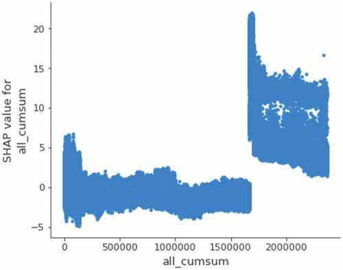
We enhanced the diversity from three aspects: model, sample and parameter. In terms of samples, we consider using two subsets of data with different numbers. The first group uses all training samples, and the second group uses part samples. As shown in Figure 2, when the cumulative number of accidents reaches a certain number, the SHAP value increases suddenly, indicating that there may be some difference between the samples. Therefore, the latter 650,000 training set samples are selected as the training samples in the second group. The adversarial verification set is also selected by means of adversarial verification.

Figure 2. Accident record cumulative SHAP values.

To increase the diversity of models and parameters, we consider using two sets of XGBoost, LightGBM, and CatBoost models with different parameters, one using the first training sample (XGB-1, LGB-1 and CB-1) and the other using the second training sample (XGB-2, LGB-2 and CB-2).

Numerical Result

Taking into account the large amount of data, MAPE is used as the objective function to establish XGBoost, LightgBM and CatBoost, and Bayesian optimization (Snoek, Larochelle, and Adams 2012) which has a great advantage when there are more hyperparameters compared with grid search or random search, is used to adjust the main hyperparameters of the models. Among them, Catboost is based on GPU training and XGBoost needs to customize the second derivative function of MAPE, it is set to $1/y_i$ here. By stacking and elastic network regression, the coefficients of XGB-1, LGB-1, CB-1, XGB-2, LGB-2 and CB-2 models are −5.666, 2.3537, −2.3233, 2.3279, 4.1241 and 4.7714, respectively. To avoid the negative value of the final feature importance, the models with negative coefficients are deleted, and the remaining models at the second layer are trained again until all coefficients are greater than 0. Finally, three models, LGB-1, LGB-2 and CB-2, are left with corresponding coefficients of 2.0805, 4.1614 and 0.8845, which are converted into weights of 0.2919, 0.5839 and 0.1241, respectively.

Since the heterogeneous ensemble learning model in this paper adopts a two-layer structure, in order to facilitate comparison, the reserved offline test set is also added to the training set when training other single models. According to the prediction results of the heterogeneous ensemble model in the test set, the average predicted duration of the accident is 51.96 minutes, the median and the standard deviation are 52.16 minutes and 6.47, respectively. Table 5 shows the final prediction effect. By heterogeneous ensemble learning, the MAPE, MAE, and MSE of the final model are 35.6101%, 30.7432, and 4252.1728, respectively. From the perspective of MAPE, heterogeneous ensemble and LightGBM are the best two models, and their effects are very close, with a difference of only about 0.15 percentage points. The MAE of heterogeneous ensemble is the best among all models. As for MSE, the objective function of heterogeneous ensemble is to minimize MAPE, and the MSE of elastic network regression is naturally minimal because of its objective function. However, we can choose or construct the loss function that meets the demand in heterogeneous ensemble, which is more flexible and convenient. Therefore, we construct the LightGBM model with MSE as the objective function to compare with the elastic network, and the results show that the MAPE, MAE and MSE of the model is 48.8222, 31.0031, 3751.3101 respectively, which are superior to the elastic network. Moreover, the MSE of heterogeneous ensemble is better than other models except elastic network regression. In general, the MAPE, MAE, and MSE of this model perform well, and its performance is the most comprehensive. More importantly, the model can combine the analysis results of factors affecting the accident duration of different models while maintaining a good predictive effect, and give the comprehensive impact of related factors, making the analysis results more referential.

Table 5. The prediction effects of different models

Model	MAPE(%)	MAE	MSE
XGBoost	36.6540	32.1356	4413.2723
LightGBM	35.4587	31.1413	4314.8268
CatBoost	36.2398	31.1533	4302.6698
Decision tree	52.9972	32.1943	6902.1944
Elastic net	60.2050	34.0313	3861.6144
Heterogeneous ensemble	35.6101	30.7432	4252.1728

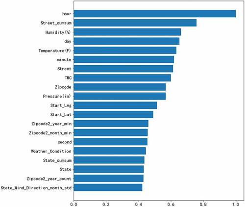
Shapley additive explanation (SHAP) values (Lundberg and Lee) is a method to solve the interpretability of the model. It can give the contribution of each factor to the duration of an individual accident, and we can use Tree SHAP (Lundberg, Erion, and Chen et al. 2020) to interpret the first-level model as an aid. In the SHAP values chart, each line represents a feature, and a dot represents a sample. The abscisaxis represents the SHAP value. The redder the color is, the larger the value of the feature itself is, while the bluer the color is, the opposite is true.

Figure 3 shows the SHAP value diagram of LGB-1. Figure 4 shows the feature importance of combinatorial models. From the perspective of the relative importance of features in the combination model, the importance of features related to accident time, accident location and weather is relatively higher, and the statistical features of structures are mainly clustered in the middle part of feature importance.

Figure 3. SHAP value.

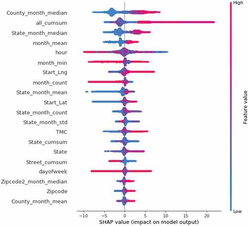
Figure 4. Feature importance of combinatorial models.

The time period of the accident is the most important for predicting the duration of the accident. Combination distribution at different times of the accident, accident occurs mainly in 6:00 to 21:00, and the incidence of accidents from around 2:00 to 4:00 is lower, but the duration is higher than in other periods. It can be seen from Figure 3 that the hour has a great positive and negative promoting effect on the predicted value of accident duration. Some sample points near 23:00 are clustered on the left side of the SHAP value graph, indicating that for this part of samples, the time period near 23:00 when the accident occurs will reduce the predicted value of the final accident duration. We speculate that the traffic flow near 23:00 is less and there are certain lighting conditions, which is convenient for the removal of the accident, thus the accident duration can be effectively shortened. However, from around 2:00 to 4:00, due to the circadian rhythm (Williamson and Friswell 2011), people tend to be tired in this period, and the light conditions are not good. Once a traffic accident occurs, it may not be conducive to the development of accident discovery and clearance, so the average duration of the accident is significantly higher than other periods. In this regard, the management should strengthen the wee morning accident detection measures, drivers should pay attention to the warning and prevention of fatigue driving.

For latitude and longitude, street accident accumulations, state accident accumulations, etc., they are related to geographical location and historical statistics. The eastern United States is more dense, and its land area is relatively small. It can be seen from SHAP value that places with large longitude and latitude mainly play a positive role in promoting the predicted value of accident duration, while places with small longitude and latitude mainly play a negative role. It means that accidents occurring in the Northeast generally increase the predicted value of accident duration. We speculate that due to high levels of urbanization and population density of the Northeast Atlantic coastal agglomerations, it is very easy to cause congestion and exceed the capacity of the road once a traffic accident occurs, making it difficult to carry out the work of accident response, clearance, rescue and traffic recovery efficiently, thus increasing accident duration. Therefore, further increasing road capacity and controlling traffic flow are effective measures to prevent accidents and reduce the duration of effective accidents.

Conclusions

Based on a large data set of more than one million incidents, we study the accident duration prediction problem in the early stage of traffic accident and construct a model of accident duration prediction based on heterogeneous integration. The model performs well and combines the advantages of multiple models, which results are more comprehensive. The results show that the time, location, weather and relevant historical statistics of the accident are important to the accident duration.

Discussions

Compared with elastic network regression, decision tree and some models, ensemble model has a greater advantage in prediction accuracy, while SVM and some models are difficult to achieve large-scale sample training. Therefore, ensemble learning is more like a balance between accuracy, efficiency and interpretability. On the one hand, considering the singleness of a single model in the analysis of influencing factors and the possible instability in the face of changes in sample distribution, the fusion of different heterogeneous models will help to give consideration to the accuracy and stability of the results. At the same time, the comprehensive analysis of the influencing factors of various models can help us grasp the main contradiction that affects the accident duration and make the conclusion more general. On the other hand, the introduction of too many models will increase the complexity of the system, so the accuracy and diversity of models need to be weighed in consideration of the efficiency cost.

In addition, since this paper focuses on the prediction of the accident duration in the early stage of traffic accidents, the information available at the early stage of accidents is limited, so too many factors cannot be included. However, with the development of the accident duration, more and more factors can be obtained and used to improve the prediction effect, but the information related to personal privacy and closely related to the accident duration is still unable to be directly used. As an innovative modeling mechanism, federated learning (Li, Sahu, and Talwalkar et al. 2020; Yang, Liu, and Chen et al. 2019) can conduct unified modeling of data from multiple parties without compromising data privacy and security and has broad application prospects in finance, medical care, smart city and other fields. Traditional methods generally pool data from multiple parties to train the model, while multiple participants can collaborate to train a machine learning model without revealing their original data in federated learning. In the field of transportation, a large number of heterogeneous data will be generated from different information sources, such as sensors, vehicles and people. Therefore, under the premise of not revealing privacy, how to integrate multi-party data through federated learning and improve the accuracy of traffic accident duration prediction is of great significance, and further research is needed.

Acknowledgment

The authors would like to thank two anonymous referees for their helpful comments.

Disclosure statement

No potential conflict of interest was reported by the author(s).

References

- Al-Deek, H., and E. B. Emam. 2006. New methodology for estimating reliability in transportation networks with degraded link capacities. Journal of Intelligent Transportation Systems 10 (3):117–1541.
- Chawla, N. V., K. W. Bowyer, L. O. Hall, et al. 2002. SMOTE: Synthetic minority over-sampling technique. Journal of Artificial Intelligence Research 16:321–57.
- Chen, T. Q., and C. Guestrin. 2016. XGBoost: A scalable tree boosting system. In Proceedings of the 22nd ACM SIGKDD International Conference on Knowledge Discovery and Data Mining, San Francisco, California, USA, 785–94.
- Cong, H., C. Chen, P. S. Lin, et al. 2018. Traffic incident duration estimation based on a dual-learning Bayesian network model. Transportation Research Record 2672 (45):196–209.
- Cover, T., and P. Hart. 1967. Nearest neighbor pattern classification. IEEE Transactions on Information Theory 13 (1):21–27.
- Demiroluk, S., and K. Ozbay. 2014. Adaptive learning in Bayesian networks for incident duration prediction. Transportation Research Record 2460 (1):77–85.
- Dimitriou, L., and E. I. Vlahogianni. 2015. Fuzzy modeling of freeway accident duration with rainfall and traffic flow interactions. Analytic Methods in Accident Research 5:59–71.
- Dowling, R., A. Skabardonis, M. Carroll, et al. 2004. Methodology for measuring recurrent and nonrecurrent traffic congestion. Transportation Research Record 1867 (1):60–68.
- Fleming, J. 2016. Adversarial validation, part one. http://fastml.com/adversarial-validation-part-one/ 2021. Accessed Jul 8, 2021.
- Friedman, J. H. 2001. Greedy function approximation: A gradient boosting machine. Annals of Statistics 29 (5):1189–232.
- Guyon, I., and A. Elisseeff. 2003. An introduction to variable and feature selection. Journal of Machine Learning Research 3 (3):1157–82.
- Hamad, K., M. A. Khalil, and A. R. Alozi. 2020. Predicting freeway incident duration using machine learning. International Journal of Intelligent Transportation Systems Research 18 (2):367–80.
- Hamad, K., R. Al-Ruzouq, W. Zeiada, et al. 2020. Predicting incident duration using random forests. Transportmetrica A: Transport Science 16 (3):1269–93.
- Haule, H. J., T. Sando, R. Lentz, et al. 2019. Evaluating the impact and clearance duration of freeway incidents. International Journal of Transportation Science and Technology 8 (1):13–24.
- Hojati, A. T., L. Ferreira, S. Washington, et al. 2013. Hazard based models for freeway traffic incident duration. Accident Analysis & Prevention 52 ():171–81.
- Hojati, A. T., L. Ferreira, S. Washington, et al. 2014. Modelling total duration of traffic incidents including incident detection and recovery time. Accident Analysis & Prevention 71:296–305.
- Jain, S. 2017. Covariate shift - unearthing hidden problems in real world data science. https://www.analyticsvidhya.com/blog/2017/07/covariate-shift-the-hidden-problem-of-real-world-data-science/. 2021. Accessed Jul 8, 2021.
- Ke, G., Q. Meng, T. Finley, et al. 2017. LightGBM: A highly efficient gradient boosting decision tree. Advances in Neural Information Processing Systems 30:3146–54.
- Khattak, A. J., J. Liu, B. Wali, et al. 2016. Modeling traffic incident duration using quantile regression. Transportation Research Record: Journal of the Transportation Research Board 2554 (1):139–48.
- Li, R., F. C. Pereira, and M. E. Ben-Akiva. 2015. Competing risks mixture model for traffic incident duration prediction. Accident Analysis & Prevention 75:192–201.
- Li, T., A. K. Sahu, A. Talwalkar, et al. 2020. Federated learning: Challenges, methods, and future directions. IEEE Signal Processing Magazine 37(3): 50–60. .
- Lin, Y., and R. Li. 2020. Real-time traffic accidents post-impact prediction: Based on crowdsourcing data. Accident Analysis & Prevention 145:105696.
- Lundberg, S. M., G. Erion, H. Chen, et al. 2020. From local explanations to global understanding with explainable AI for trees. Nature Machine Intelligence 2 (1):56–67.
- Lundberg, S. M., and S. I. Lee. 2017. A unified approach to interpreting model predictions. In Proceedings of the 31st International Conference on Neural Information Processing systems, Long Beach, California, USA, 4768–77.
- Ma, X., C. Ding, S. Luan, et al. 2017. Prioritizing influential factors for freeway incident clearance time prediction using the gradient boosting decision trees method. IEEE Transactions on Intelligent Transportation Systems 18 (9):2303–10.
- Mfinanga, D., and E. Fungo. 2013. Impact of incidents on traffic congestion in Dar es Salaam city. International Journal of Transportation Science and Technology 2 (2):95–108.
- Micci-Barreca, D. 2001. A preprocessing scheme for high-cardinality categorical attributes in classification and prediction problems. ACM SIGKDD Explorations Newsletter 3 (1):27–32.
- Moosavi, S., M. H. Samavatian, S. Parthasarathy, et al. A countrywide traffic accident dataset. arXiv preprint arXiv:2019a, preprint arXiv.
- Moosavi, S., M. H. Samavatian, S. Parthasarathy, et al. 2019b. Accident risk prediction based on heterogeneous sparse data new dataset and insights. In Proceedings of the 27th ACM SIGSPATIAL International Conference on Advances in Geographic Information Systems, Chicago, Illinois, USA, 2019b33–42.
- Moreno-Torres, J. G, T. Raeder, R. Alaiz-Rodríguez, et al. 2012. A unifying view on dataset shift in classification. Pattern Recognition 45 (1):521–30.
- Nam, D., and F. Mannering. 2000. An exploratory hazard-based analysis of highway incident duration. Transportation Research Part A: Policy and Practice 34 (2):85–102.
- Ozbay, K., and N. Noyan. 2006. Estimation of incident clearance times using Bayesian networks approach. Accident Analysis & Prevention 38 (3):542–55.
- Prokhorenkova, L., G. Gusev, A. Vorobev, et al. 2017. CatBoost: Unbiased boosting with categorical features. arXiv preprint arXiv:1706.09516.
- Raschka, S. 2015. Python machine learning. Birmingham, UK: Packt publishing ltd.
- Snoek, J., H. Larochelle, and R. P. Adams. 2012. Practical Bayesian optimization of machine learning algorithms. Advances in Neural Information Processing Systems 25:2960–68.
- Stekhoven, D. J., and P. Bühlmann. 2012. MissForest—non-parametric missing value imputation for mixed-type data. Bioinformatics 28 (1):112–18.
- Tang, J., L. Zheng, C. Han, et al. 2020. Traffic incident clearance time prediction and influencing factor analysis using extreme gradient boosting model. Journal of Advanced Transportation 2020 (1):1–12.
- Valenti, G., M. Lelli, and D. Cucina. 2010. A comparative study of models for the incident duration prediction. European Transport Research Review 2 (2):103–11.
- Wang, X., S. Chen, and W. Zheng. 2013. Traffic incident duration prediction based on partial least squares regression. Procedia - Social and Behavioral Sciences 96:425–32.
- Williamson, A., and R. Friswell. 2011. Investigating the relative effects of sleep deprivation and time of day on fatigue and performance. Accident Analysis & Prevention 43 (3):690–97.
- Wolpert, D. H. 1992. Stacked generalization. Neural Networks 5 (2):241–59.
- Yang, Q., Y. Liu, T. Chen, et al. 2019. Federated machine learning: Concept and applications. ACM Transactions on Intelligent Systems and Technology (TIST) 10 (2):1–19.
- Zheng, A., and A. Casari. 2018. Feature engineering for machine learning: Principles and techniques for data scientists. Sebastopol, California, USA: O'Reilly Media, Inc.
- Zou, H., and T. Hastie. 2005. Regularization and variable selection via the elastic net. Journal of the Royal Statistical Society: Series B (Statistical Methodology) 67 (2):301–20.