A Homogeneous Ensemble Classifier for Breast Cancer Detection Using Parameters Tuning of MLP Neural Network

ABSTRACT

Breast cancer is one of the most common cancers among worldwide, and its detection is recognized as a significant public health problem in today’s society. Extensive studies have been conducted to classify patients into malignant or benign groups, but given the importance of the problems, efforts are still ongoing. This paper aims are to parameters tuning of Multi-Layer Perceptron (MLP) neural network for the breast cancer detection. This work presents an MLP-based homogeneous ensemble approach for classifying breast cancer samples. Basically, ensemble learning is used to improve the classification process. This technique is a method of combining different basic classifiers from which a new classifier is derived. In this regard, several optimization algorithms including GA, PSO, and ODMA have been used to determine which algorithm provides the most suitable parameters for MLP. These parameters include effective features, number of hidden layers, number of nodes in layers, and weight values. The proposed algorithm is applied to three datasets of the Wisconsin Breast Cancer Database (i.e., WBCD, WDBC, and WPBC) and then comparison is made between different algorithms to achieve the highest accuracy. Experiments show that the proposed classifier has promising results in breast cancer detection than other state-of-the-art classifiers with 98.79% in the WBCD. Data analysis and its results can confirm the superiority of ensemble classifiers over state-of-the-art methods for breast cancer detection.

Introduction

Global cancer statistics show that of the 19.3 million new cases of cancer in 2020, breast cancer in women will affect about 2.3 million, or 12%, while lung cancer accounts for 11% (Ahmad et al. 2015; Pati et al. 2021). The burden of cancer as one of the leading causes of death and an important barrier to life expectancy is increasing rapidly around the world (Ibrahim and Shamsuddin 2018). The science of data mining discovers hidden and unknown patterns among the vast amount of data that are sometimes hidden from the view of medical professionals (Bilalović and Avdagić 2018). In the meantime, various methods have been used to predict the survival and recurrence of breast cancer patients, and sometimes their results have supported the decisions of physicians (Bilalović and Avdagić 2018; Ibrahim and Shamsuddin 2018; Singla, Ghosh, and Kumari 2019). These methods are not supposed to replace the decisions of experts and researchers, but by using specific and repetitive patterns, they can help them in sensitive situations (Singla, Ghosh, and Kumari 2019). In general, data mining focuses on the implementation of various classification methods to predict breast cancer (malignant or benign).

According to the above requirements, data mining methods can be used to facilitate the improvement of diagnostic systems. Automatic detection systems can reduce the potential for physicians to make mistakes during diagnosis (Abdar and Makarenkov 2019). Selecting the most important features is one of the most important tasks in designing a classification model. Therefore, to build an efficient automated diagnosis system for breast cancer diagnosis, there is a need for a way to select important features. Optimization algorithms (Ghobaei-Arani et al. 2019; Khorsand, Ghobaei‐Arani, and Ramezanpour 2018) such as Genetic Algorithm (GA) are known as a tool to determine the dependence of information and reduce the number of features (Bilalović and Avdagić 2018). The new dataset obtained after the application of optimization algorithms is considered as input to the classification models, where it has smaller dimensions than the original dataset (Bilalović and Avdagić 2018). Therefore, the best subset of features is used as input to different classification models. Classification models use mathematical techniques such as statistics, neural networks, linear programming, and decision trees for classification (Khorsand, Ghobaei‐Arani, and Ramezanpour 2019). In other words, classification is the process of finding a model that describes data classes and concepts and divides the data into specific groups (Abdar and Makarenkov 2019). Today, various classification models in the field of data mining based on medical data have been introduced (Ibrahim and Shamsuddin 2018). However, the performance of each algorithm depends on different model configurations, such as a variety of input features and model parameters. To address the performance limitations of single models, we use an ensemble classification model to diagnose breast cancer. Ensemble classification use a combination of several individual classifiers, each building its own model on the data and storing that model (Ontiveros-Robles and Melin 2020).

Data mining techniques can help doctors make the right decision to diagnose breast cancer (Singla, Ghosh, and Kumari 2019). In this regard, we use different data mining methods to diagnose breast cancer. In this paper, the use of feature selection approaches and classification models is emphasized. The effective features selection eliminates insignificant features (Narvekar et al. 2019; Yavuz and Eyupoglu 2020). Here, various optimization algorithms are used to do this. The process of effective features selection reduces computational complexity and speeds up the data mining process. In addition, we use an ensemble classification model to produce an accurate system for predicting breast cancer. The proposed model is based on MLP and is evaluated by combining different techniques. The importance of MLP is in setting its parameters, where we use optimization algorithms to set these parameters. Therefore, in addition to the effective features, the parameters that are optimized include number of hidden layers, number of nodes in layers, and weight values.

The main contribution of this paper is as follows:

• Development of optimization algorithms for tuning MLP neural network parameters

• Design of a homogeneous ensemble classification framework based on the tuning of neural network parameters

The rest of the paper is as follows: Section 2 is dedicated to the background. Section 3 lists related works. Section 4 provides an explanation of the proposed method. The simulations and comparison results are discussed in Section 5. Finally, the conclusion is given in Section 6.

Background

In this section, the methods used in this paper are reviewed. These methods include classification concepts, MLP neural networks, and optimization algorithms.

Ensemble Classification Concepts

So far, many classification models have been proposed, but none have been the best in all respects (Hazra, Mandal, and Gupta 2016). In order to reduce the impact of this problem, ensemble-based classification techniques are proposed. This technique can do the learning work based on a group of single classification models. Ensemble-based classification by combining the prediction results of each single model can provide the final prediction with better accuracy. This is achieved by learning the errors of each of the single classification models (Hazra, Mandal, and Gupta 2016). The way it is done is defined in the two techniques: Bagging and Boosting. Bagging is a method of merging the same type of predictions. Boosting is a method of merging different types of predictions. Basically, Bagging and Boosting techniques are used to create ensemble classification models. Bagging is a method of merging the same type of predictions. Boosting is a method of merging different types of predictions. Here, learning is done based on the single classifier models $c_1,c_2,\dots ,c_q$ and then a meta-classifier is learned that combines the outputs.

MLP Neural Network

Multilayer perceptron neural networks (MLPs) are a class of feedforward artificial neural networks (Yavuz et al. 2017). In MLP, there are at least three layers of nodes: input layer, hidden layer and output layer (Mohammed et al. 2018). In this MLP, the output of the first layer (i.e., input) is essentially the input of the next layer (i.e., hidden). In this regard, the output of each hidden layer is used as the input of the next hidden layer. Finally, the output of the last hidden layer is combined as the input of the output layer to finally display the prediction results in the output layer. All the layers that are placed between the input layer and the output layer are called hidden layers. The MLP also contains a set of weights that must be set for network training and learning (Mohammed et al. 2018). At each stage, one of the input data enters the neural network. With a set of weights and bias values, the MLP can produce output tailored to the input data and weights. The output in the last layer is called predicted output. In all supervised learning algorithms, the actual output of the training data is predetermined. Expected outputs are used to measure MLP performance. In this way, based on the expected output and predicted output values, the loss value is calculated. The loss value is then inverted in the network, and weights are updated using a concept such as Gradient.

Optimization Algorithms

Along with the increasing popularity of optimization methods in various sciences, researchers have also used these methods for various purposes. Optimization methods use basic methods and operations to solve the problem and reach a suitable solution to the problem during a series of iterations. Due to the use of optimization methods for tuning MLP parameters, some optimization methods are briefly described below.

Genetic Algorithm (GA)

This algorithm proposed by Holland (1992), essentially form the foundations of modern evolutionary computing. GA use the genetic operators: selection, mutation, and crossover (Abdel-Basset et al. 2020). Each solution (as a chromosomes) is encoded as a string of gens. The crossover of two selected parent produces offspring by swapping genes of the chromosomes. Mutation typically works by making small changes at random to an individual’s genome. After the mutation phase, the generation of genetic iteration is complete. The process goes on until we reach the termination condition.

Particle Swarm Optimization (PSO)

This algorithm was proposed by Kennedy and Eberhart (1995). Using existing social models and social relationships, they developed a type of computational intelligence that had special abilities to solve optimization problems. This method is adapted from the collective performance of groups of animals, such as birds and fish. There are a number of organisms in PSO, which are called particles. By scattering particles in the search space, the values of the objective function are calculated according to the position of each particle. Then, using the combination of the current position, the best position ever obtained (i.e., $pbest$), and the best position in the whole population (i.e., gbest), each particle updates its position. After performing the group move, one step of the algorithm is completed. This process is repeated until the desired solution is obtained and one or more stop conditions are estimated.

Open-Source Development Model Algorithm (ODMA)

This algorithm was proposed by Hajipour, Khormuji, and Rostami (2016) to solve complex real-world optimization problems. ODMA is known as a metaheuristic approach that performs population optimization and evolution based on an open-source development model. Each member in ODMA is known as a software that the evolution process seeks to develop and improve software. In general, ODMA categorizes the population of software into two groups, leading and promising, which are the leading group of software with the highest fitness function. The ODMA evolution phase consists of three toast phases. In the first phase, each software moves toward a leading software. In the second phase, leading software is developed based on its history. Finally, forking of the leading software in the third phase is done.

Related Works

So far, methodologies based on ensemble classification models for predicting and diagnosing breast cancer have been introduced by researchers (El Ouassif, Idri, and Hosni 2021; Rezaeipanah and Ahmadi 2020; Talatian Azad, Ahmadi, and Rezaeipanah 2021; Zhu et al. 2019). In this section, we systematically review and analyze some of the most recent research papers related to breast cancer diagnosis. Recently, in (Zhu et al. 2019), an ensemble deep learning approach has been used to classify breast cancer molecular groups. In this paper, Random Forest (RF) ensemble and Extra Trees (ET) ensemble techniques for classifying WBCD datasets are compared and investigated. In (Talatian Azad, Ahmadi, and Rezaeipanah 2021), MLP neural network and evolutionary algorithms have been used to create an ensemble classification model to predict breast cancer. In (El Ouassif, Idri, and Hosni 2021), homogeneous ensemble based on four types of Support Vector Machines (SVM) classifiers has been evaluated for the breast cancer diagnosis. Here, four SVMs use different kernels, including the linear, normal polynomial, radial base function, and Pearson VII function. In addition, MLP is used to combine the output of the base classifiers. In (Rezaeipanah and Ahmadi 2020), the diagnosis of breast cancer using multi-stage weight adjustment in the MLP neural network has been proposed.

In (Wang et al. 2018), an SVM-based ensemble algorithm for breast cancer diagnosis is proposed. Here, 12 different SVM are combined on a weighted area under the receiver characteristic curve model. In this algorithm, the accuracy of breast cancer diagnosis is significantly increased by 97.89%. In (Kadam, Jadhav, and Vijayakumar 2019), breast cancer diagnosis was performed using feature ensemble learning based on stacked sparse autoencoders and SoftMax regression. The prediction results obtained by this algorithm with a true accuracy of 98.60% are very promising. In (Abdar et al. 2020), a new nested ensemble technique for automatic detection of breast cancer is proposed. Here, both voting and stacking techniques have been used to build nested ensemble model, where results on the Wisconsin Diagnostic Database (WDBC) show the superiority of the stacking technique with an accuracy of 98.07%. In (Idri, Hosni, and Abnane 2020), the effect of parameter adjustment in ensemble based on breast cancer classification has been evaluated. Here, the classification of heterogeneous ensembles is developed based on three machine learning methods (SVM, MLP, and decision trees). The authors compared three parameters tuning methods including PSO, Grid Search (GS), and the default parameters of the Weka. Plus, the heterogeneous ensembles of this study were built using the majority voting technique. Finally, a comparison of studies for breast cancer prediction with approaches is presented in Table 1.

Table 1. Comparison of existing techniques for breast cancer detection

Reference	Methods	Advantages	Disadvantages	Results
Zhu et al. (2019)	Investigation of deep learning for differentiation between molecular subtypes of breast cancer	The C4.5 has been introduced as the most widely used approach to cancer diagnosis	Basic and statistical criteria were not used in the comparisons	-
Talatian Azad, Ahmadi, and Rezaeipanah (2021)	An intelligent ensemble classification method based on neural network	Stacked generalization-based ensemble classification improves model prediction results	Simultaneous optimization of parameters increases the complexity of the GA	98.74%
El Ouassif, Idri, and Hosni (2021)	Homogeneous ensemble based on four types of SVM classifiers	Using the Borda Count to rank the best classifiers	The effect of parameter tuning on classification performance has not been investigated	90.88%
Rezaeipanah and Ahmadi (2020)	Using multi-stage weight adjustment in the neural network	Find the best MLP structure by performing simultaneous and automatic search	There is no comparison with single classification models	98.74%
Wang et al. (2018)	An SVM-based ensemble algorithm	Using large real datasets to perspectives of model effectiveness	Feature selection techniques have not been used to reduce model complexity	97.89%
Kadam, Jadhav, and Vijayakumar (2019)	Using of feature ensemble learning based on stacked sparse autoencoders	Using the integration of different classifiers to benefit from the representation of all layers	Comparing the rules to make a final decision lacks statistical analysis	98.60%
Abdar et al. (2020)	A novel nested ensemble technique based on voting and stacking	Using the two-layer nesting ensemble technique improves the performance	No approach has been proposed to deal with high-dimensionality and large data volumes	98.07%
Idri, Hosni, and Abnane (2020)	Heterogeneous ensembles classification based on SVM, MLP, and ID3	Improving heterogeneous ensemble techniques developed based on the Borda Count method	The complexity is relatively high due to the lack of feature selection approaches	95.90%

The Proposed Method

For classification work, it is not possible to provide a single classification model that performs better in any situation (Kadam, Jadhav, and Vijayakumar 2019). Therefore, to improve the performance of classifications, ensemble classifications have recently attracted more attention. In general, ensemble learning methods include two types of homogeneous and heterogeneous (Abdar et al. 2020). In homogeneous all models used in the classification process are the same. These methods can create variation by dividing samples between models, although they do the learning process based on a basic classification algorithm. In addition, in heterogeneous all models used in the classification process are different. Therefore, these methods use different basic classification algorithms for learning work. Diversity in heterogeneous ensemble learning can be created through the use of different classifications, where the data are the same for each model. In this regard, homogeneous methods can use a feature selection approach for each part of the data. However, heterogeneous methods can have different approaches to feature selection.

After determining how the classifiers are combined, a mechanism must be selected to combine their output results. This mechanism can make the final decision for classification. So far, many mechanisms have been proposed for this, including majority vote, average, meta-classifiers, Borda-Count and Dempster-Shafer (Talatian Azad, Ahmadi, and Rezaeipanah 2021). In this paper, meta-classifiers are used to combine classifiers and Stacking is used to create ensemble classification. As noted above, stacking has become a commonly used technique for generating ensembles of heterogeneous classifiers. The architecture of the proposed algorithm is shown in Figure 1.

Figure 1. The architecture of the proposed algorithm.

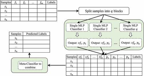
In this paper, MLP-based homogeneous ensembles are used to diagnose breast cancer. Here, MLP parameters are tuned based on optimization algorithms. Optimization is based on GA, PSO, and ODMA, where the purpose of evaluating these algorithms is to find the best parameters. These parameters include effective features, number of hidden layers, number of nodes in layers, and weight values. First, we divide all the samples in the training dataset into q blocks, so that all the blocks are the same size. Then, $c_i,\mathrm{\forall }i=1,2,\dots ,q$ single MLP classifier is trained on $b_i,\mathrm{\forall }i=1,2,\dots ,q$ data block. At this stage, each MLP is trained separately by an optimization algorithm to find the optimal parameters. This process creates homogeneous classification models according to the Stacking technique. Next, we create a new dataset based on the output of the training phase, where this dataset is considered as the meta-classifier input. Here, the meta-classifier is an MLP that is taught similar to the previous step by an optimization algorithm. Therefore, we use the meta-classifier technique to combine the output of single classifiers. Figure 2 shows the flowchart of the proposed method.

Figure 2. Flowchart of the proposed method.

In the proposed method, the new dataset generated from the training phase has different features. For example, based on the classifier $c_i$, $s{f}_i$ (subset of selected features) and $p_i$ (predictive samples label) can be considered as features in the new dataset. Accordingly, the details of the features of this dataset can be represented as $\left\{\cup (s{f}_1,s{f}_2,\dots ,s{f}_q),p_1,p_2,\dots ,p_q\right\}$, where $\cup$ is a union operator. In this regard, we also store the actual label for each sample in this dataset. The new data sets generated for the training work are used by the meta-classifier mechanism. Classification models are configured based on several optimization methods (i.e., GA, PSO, and ODMA). Each optimization method has components, such as solution representation structure, initial population creation, fitness function, evolutionary operators, and iteration stop conditions. In general, for all optimization methods, all parts are the same except for evolutionary operators. In the following, we will explain in detail the optimization methods for configuring the MLP neural network. The solution representation structure is used as a way to encode each solution in the population. In this paper, the structure of each solution has three sections of selected features, hidden layers, and weight values, as shown in Figure 3.

Figure 3. Solutions representation structure.

Here, the selected features are given in the first part of the solution and the second part shows the details of the hidden layers, where $w$ represents the maximum number of hidden layers and $m$ is the total number of features. In this regard, the values assigned to the weights are given in the third part of the solution, where the total number of weights is determined based on the structure of the MLP neural network. Meanwhile, $f_i\in \left[0,1\right]$ is indexed to feature $i$, $h_j\in \left[0-10\right]$ refers to the number of nodes in hidden layer $j$, and $w_k\in \left[-1,+1\right]$ is the communication weight in MLP. In this regard, the solution length in the structure is $D=m+w+v$. Accordingly, the initial population is randomly generated. Typically, MLP follows a supervised learning approach to training. Therefore, we consider the classification error (MAE) as a fitness function. In addition to error, the complexity of the MLP neural network is also defined as fitness function. In general, fewer connections in MLP reduce the complexity of the classification model. Therefore, fitness function is defined as multi-objective according to Eq. (1)(1) $Fitness=MAE+\left(\alpha .\beta +\beta .\gamma +\beta +\gamma \right)$(1) .

(1) $Fitness=MAE+\left(\alpha .\beta +\beta .\gamma +\beta +\gamma \right)$(1)

Where, $\alpha$ is the number of selected features, $\beta$ is the number of hidden layers in the MLP neural network, and $\gamma$ refers to the size of the output nodes. Here, network complexity is defined based on (Ahmad et al. 2015) and the purpose is to minimize the fitness function. In addition, the termination condition is to reach a fixed maximum number. The following are the details of evolutionary operators for each of the optimization algorithms.

Details of Evolutionary Operators for GA

GA uses three operators to evolve the population and perform optimizations (i.e., selection, crossover, and mutation). The following are the details of these operators for tuning neural network parameters.

Selection

This operator is used to select the appropriate chromosomes from the population and ultimately reproduce. In this paper, the roulette wheel mechanism (Ghalehgolabi and Rezaeipanah 2017) is used for this purpose, where Eq. (2)(2) $P_i=\frac{ob{j}_i}{{\sum }_{i=1}^{N_{Pop}}ob{j}_i}$(2) shows the process of calculating the probability of selecting the $i$-th chromosome.

(2) $P_i=\frac{ob{j}_i}{{\sum }_{i=1}^{N_{Pop}}ob{j}_i}$(2)

Where, $ob{j}_i$ is the fitness value of $i$-th chromosome and $N_{Pop}$ is related to the number of members of the population.

Crossover

This operator is used for reproduction. In this paper, Differential Evolution (DE) is used as a crossover operator (Ghalehgolabi and Rezaeipanah 2017). DE can possibly apply CR to selected chromosomes (parents) and produce a new chromosome (offspring). Because the solution representation structure has different sections, here DE is applied to each section independently. The DE technique performs the offspring production process (e.g., $X^O$) based on $X^0$, $X^1$ and $X^2$. According to the equation, the process of calculating $X^O$ is based on measuring the weight difference between and $X^2$ and adding its value to $X^0$.

(3) $x_i^O=\left\{\begin{array}{cc}{x}_i^0+F.\left(x_i^1-x_i^2\right)& CR>Rnd\left(0,1\right)\\ x_i^0& otherwise\end{array}\right.$(3)

Where, $X^1$ refers to the first parent selected and $X^2$ is the second parent selected for reproduction. Also, $X^0$ is the best chromosome based on the fitness function. In addition, $F\in \left(0,1\right)$ is used as a coefficient to control evolution in the population.

In general, using a constant coefficient as the value of $F$ creates an outside between the values of different parts of the chromosome. Therefore, in this paper, $F$ is dynamically defined based on Eq. (4)(4) $F=\frac{\alpha .Rnd\left(0,1\right)}{max\left(x_{i,g}^1,x_{i,g}^2\right)}$(4) .

(4) $F=\frac{\alpha .Rnd\left(0,1\right)}{max\left(x_{i,g}^1,x_{i,g}^2\right)}$(4)

where, $\alpha$ is considered as the scale factor and has a value less than 1. Also, $g$ refers to the generation to which the chromosome belongs.

Mutation

This operator is used to apply genetic diversity and mutations to a child’s chromosome. In this paper, Bit Change (BC) (Ghalehgolabi and Rezaeipanah 2017) is used as a mutant that is applied to each element of the chromosome with a probability of MR. The BC mutation operator is defined based on the Eq. (5)(5) $x_i^{OM}=\left\{\begin{array}{cc}{x}_i^O+\mathrm{\Delta }& MR>Rnd\left(0,1\right)\\ x_i^O& otherwise\end{array}\right.$(5) .

(5) $x_i^{OM}=\left\{\begin{array}{cc}{x}_i^O+\mathrm{\Delta }& MR>Rnd\left(0,1\right)\\ x_i^O& otherwise\end{array}\right.$(5)

Where, $X^{OM}$ is the output chromosome after mutation and $\mathrm{\Delta }$ is the range that determines the random changes of the mutation operator on the chromosome.

Details of Evolutionary Operators for PSO

The position of a particle is denoted by $X_i=\left\{x_{i,1},x_{i,2},\dots ,x_{i,D}\right\}$, where $D$ refers to the dimensions of the solution. In addition to position, each particle has a velocity vector denoted by $V_i=\left\{v_{i,1},v_{i,2},\dots ,v_{i,D}\right\}$. In each iteration, the PSO can update the position and velocity vector of each particle based on ‘$pbest{ }^{\mathrm{\prime }}$ and ‘$gbest{ }^{\mathrm{\prime }}$, as given in the Eq. (6)(6) $v_k^{t+1}=\omega .v_k^{t+1}+c_1.r_1.\left(pbes{t}_k-x_k^t\right)+c_2.r_2.\left(gbest-x_k^t\right)$(6) and (7(7) $x_k^{t+1}=x_k^t+v_k^{t+1}$(7) ).

(6) $v_k^{t+1}=\omega .v_k^{t+1}+c_1.r_1.\left(pbes{t}_k-x_k^t\right)+c_2.r_2.\left(gbest-x_k^t\right)$(6)

(7) $x_k^{t+1}=x_k^t+v_k^{t+1}$(7)

Where, $\omega$ is the weight of inertia that controls the velocity fluctuation, $c_1$ and $c_2$ are the acceleration constants, and $r_1$ and $r_2$ are random values in the range [0,1].

In general, PSO is used to solve continuous problems. However, versions of this algorithm for solving discrete problems are also provided. For example, Kennedy and Eberhart (1995) introduced the Binary PSO (BPSO), which represents the position vector for each particle based on a binary string. In this method, the position of the particles is updated according to the Eq. (8(8) $x_k^{t+1}=\left\{\begin{array}{cc}1& Rnd\left(0,1\right)<\frac{1}{1+e^{-v_k^{t+1}}}\\ 0& otherwise\end{array}\right.$(8) ), where $x_k^{t+1}$ is restricted to 0 or 1 based on the sigmoid function.

(8) $x_k^{t+1}=\left\{\begin{array}{cc}1& Rnd\left(0,1\right)<\frac{1}{1+e^{-v_k^{t+1}}}\\ 0& otherwise\end{array}\right.$(8)

Accordingly, is mapped to a binary value using the sigmoid function, because in the feature selection section ‘0’ indicates no feature selection and ‘1’ refers to feature selection. However, other parts of the solution do not have binary features. Accordingly, Eq. (9)(9) $x_k^{t+1}=\left\{\begin{array}{cc}{x}_k^t+\mathrm{\Delta }& Rnd\left(0,1\right)<\frac{1}{1+e^{-v_k^{t+1}}}\\ x_k^t& otherwise\end{array}\right.$(9) is used for the layers and weights.

(9) $x_k^{t+1}=\left\{\begin{array}{cc}{x}_k^t+\mathrm{\Delta }& Rnd\left(0,1\right)<\frac{1}{1+e^{-v_k^{t+1}}}\\ x_k^t& otherwise\end{array}\right.$(9)

where, $\mathrm{\Delta }$ shows the rate of changes made to the previous position in order to create a new position.

Details of Evolutionary Operators for ODMA

According to ODMA, solutions are sorted by the value of the ascending fitness function. Then, $z$ solutions with the highest fitness function are selected as the leading solutions, while other solutions are selected as promising solutions. In the first stage, promising solutions are developed based on leading solutions. To do this, for each promising solution, a leading solution is selected based on the fitness function, and the evolution process is performed based on the coefficient $\rho$, as shown in Eq. (10)(10) $\begin{array}{cc}{ }_k^{pm}=\left\{\begin{array}{cc}{S}_k^{ld}& \rho >Rnd\left(0,1\right)\\ S_k^{pm}& otherwise\end{array}\right.,& \mathrm{\forall }k=1,2,\dots ,D\end{array}$(10) .

(10) $\begin{array}{cc}{ }_k^{pm}=\left\{\begin{array}{cc}{S}_k^{ld}& \rho >Rnd\left(0,1\right)\\ S_k^{pm}& otherwise\end{array}\right.,& \mathrm{\forall }k=1,2,\dots ,D\end{array}$(10)

where, $S^{pm}$ is the promising solution that moves toward the $S^{ld}$ leading solution. This process is performed for each element of the solution, such as $k$. Here, a bed of the boundaries of each part of the solution is considered.

In the second stage, leading solutions evolve based on their history. Here, evolution is based on the current position ($S^{cur}$) and the previous position ($S^{old}$) of a leading solution. Hence, $S^{new}$ new position is the leading solution, as shown in Eq. (11)(11) $\begin{array}{cc}\begin{array}{c}\begin{array}{c}{S}_k^{new}=\frac{S_k^{cur}+S_k^{old})}{2}+R,\end{array}\end{array}& \mathrm{\forall }k=1,2,\dots ,D\end{array}$(11) .

(11) $\begin{array}{cc}\begin{array}{c}\begin{array}{c}{S}_k^{new}=\frac{S_k^{cur}+S_k^{old})}{2}+R,\end{array}\end{array}& \mathrm{\forall }k=1,2,\dots ,D\end{array}$(11)

where, $∥\ast ∥$ is used to round the number and $R$ is a random number generator between $\left[-1,+1\right]$.

In the third stage, new solutions are produced based on the leading solutions. Here, a number of weak solutions with minimal progress (minimum fitness function) are eliminated and replaced by new solutions. Eq. (12)(12) $\begin{array}{cc}\begin{array}{c}\begin{array}{c}{S}_k^{new}=S_k^{ld}+R,\end{array}\end{array}& \mathrm{\forall }k=1,2,\dots ,D\end{array}$(12) shows the process of generating a new solution from a leading solution.

(12) $\begin{array}{cc}\begin{array}{c}\begin{array}{c}{S}_k^{new}=S_k^{ld}+R,\end{array}\end{array}& \mathrm{\forall }k=1,2,\dots ,D\end{array}$(12)

where, $R$ is a random number for neighborhood search. In addition, in all three stages, non-violation of the bands of each part of the solution is considered.

Results and Discussion

In this section, extensive simulations and comparisons are performed to evaluate the proposed algorithm. Here, the simulation is performed using MATLAB R2019a. An Acer Laptop with an Intel® Core^TM i5 processor at 3.0 GHz and 8 GB of memory has been used for simulation work. In addition, we report the results of the proposed model and other comparable methods based on an average of 20 separate runs to be reliable.

In a neural network, the activation function is responsible for transforming the summed weighted input from the node into the activation of the node or output for that input. In this paper, we use the rectified linear activation function. The rectified linear activation function is a piecewise linear function that will output the input directly if it is positive, otherwise, it will output zero. In addition, to perform the simulation, the parameters of the proposed algorithm are set as follows:, $w=5$, $N_{pop}=30$, $Ite{r}_{max}=500$, $CR=0.8$, $MR=0.1$, $\alpha =0.15$, $\omega =0.7$, $c_1=c_2=0.5$, $\rho =0.35$. Here, some initial parameter values are obtained from similar studies (Rezaeipanah and Ahmadi 2020; Talatian Azad, Ahmadi, and Rezaeipanah 2021). Other parameters of the proposed algorithm are optimized using Taguchi method (Azadeh et al. 2017).

Breast Cancer Dataset

The Wisconsin Breast Cancer Database (WBCD) from the UCI repository has been widely used in experiments for breast cancer diagnosis. The WBCD dataset consists of 699 samples and 9 features. In addition to WBCD, the performance of the proposed algorithm is evaluated on other Wisconsin datasets, including Wisconsin Diagnostic Breast Cancer (WDBC) and Wisconsin Prognostic Breast Cancer (WPBC). WDBC consists of 569 samples and 31 features and WPBC has 198 samples and 34 features. Meanwhile, the missing values in these datasets are replaced by the average value.

Performance Analysis

The model created by the training set should be evaluated and analyzed by the testing set. Based on this analysis, the performance of a learning algorithm is evaluated. In order to evaluate a classification model, original labels in the dataset and predicted labels from the model are used. For a two-class classification model, different prediction states are provided by the symbols True Positive (TP), True Negative (TN), False Positive (FP), and False Negative (FN) (Forouzandeh, Rostami, and Berahmand 2021; Rezaeipanah and Ahmadi 2020). Evaluation criteria are calculated based on these symbols. In this paper, the criteria of accuracy, sensitivity, and specificity are used to evaluate the proposed algorithm. These criteria are defined in Eq. (13)(13) $Accuracy=\frac{TP+TN}{TP+FP+TN+FN}$(13) , (14(14) $Sensitivity=\frac{TP}{TP+FN}$(14) ) and (15(15) $Specificity=\frac{FP}{TP+FP}$(15) ).

(13) $Accuracy=\frac{TP+TN}{TP+FP+TN+FN}$(13)

(14) $Sensitivity=\frac{TP}{TP+FN}$(14)

(15) $Specificity=\frac{FP}{TP+FP}$(15)

In addition to these criteria, we use the number of features used in the modeling, the number of connections in the MLP, and the runtime (s) to evaluate the proposed method. In this regard, evaluation criteria are calculated and presented based on 10-fold cross validation.

Proposed Algorithm Analysis

In this section, various experiments are performed to evaluate the proposed algorithm. In the first experiment, the effectiveness of GA, PSO, and ODMA algorithms for tuning MLP parameters is investigated. This review is based on the number of features selected and the importance of the features in Figure 4 for the WBCD dataset. This comparison for the WDBC and WPBC datasets is given in Figures 5 and 6, respectively. Due to the high dimensions of the WDBC and WPBC datasets, for better clarity the results are reported for only 10 important features.

Figure 4. Evaluation of different algorithms in tuning MLP parameters on the WBCD dataset.

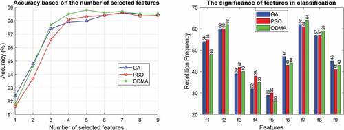
Figure 5. Evaluation of different algorithms in tuning MLP parameters on the WDBC dataset.

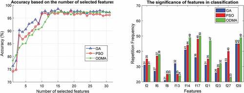
Figure 6. Evaluation of different algorithms in tuning MLP parameters on the WPBC dataset.

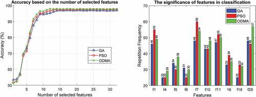
In the proposed algorithm, in addition to the subset of effective features, their number is also determined automatically by the optimization algorithm. The results presented on the WBCD show that the best accuracy of 98.79% with 5 effective features is achieved by ODMA. Meanwhile, GA and PSO are in the next ranks both with seven features as well as 98.59% and 98.57% accuracy, respectively. The results for WDBC and WPBC are similar and excellence is achieved by ODMA. Accordingly, ODMA with 16 features has reached 98.52% accuracy on WDBC and these results have been achieved for WPBC with only 12 features and 97.92% accuracy.

In addition, important features are estimated based on the number of presence (repetition frequency) in the optimization process. The results for all three optimization algorithms clearly show that features $f_2$, $f_7$ and $f_8$ are among the most important features in the WBCD for breast cancer diagnosis. However, ODMA has highlighted the importance of these features. The results are similar for WDBC and WPBC, and ODMA better demonstrates the importance of features. In WDBC, important features are $f_{14}$, $f_{17}$, and $f_{29}$, and features $f_7$, $f_{11}$, and $f_{28}$ in WPBC are more important in diagnosing breast cancer. Due to the superiority of ODAM, the following results are reported based on this algorithm.

Basically, the number of single models used to create an ensemble classification is important. The proposed algorithm with different number of single classifications is investigated. Studies show that for all three datasets, the use of four single classifications provides better performance.

In the next experiment, we evaluate the effectiveness of the proposed algorithm in detecting cancer in cases with and without feature selection (FS). The results of this comparison are shown in Table 2 for the proposed algorithm and the three datasets examined. The results show the significant superiority of the proposed algorithm with the feature selection process. Therefore, the proposed algorithm of irrelevant features can be eliminated without affecting the learning performance. In addition, due to the smaller selected features, the complexity of the network is reduced by feature selection, where the value of the number of connections is more than doubled when no feature selection is used.

Table 2. Performance of proposed algorithm with/without features selection

Criterion	With FS	Without FS	With FS	Without FS	With FS	Without FS
	WBCD		WDBC		WPBC
No. of selected features	4.8	9.0	15.5	31	12.1	34
No. of connections	36.7	100.4	83.4	308.5	68.0	325.8
Accuracy (%)	98.79	98.61	98.52	98.11	97.92	97.76
Sensitivity (%)	99.30	98.48	97.75	97.34	97.40	97.32
Specificity (%)	98.44	98.23	99.05	98.64	98.22	98.36
F1 score (%)	97.74	97.81	97.98	98.40	98.35	98.87
Runtime (s)	63.1	64.8	125.9	133.7	78.6	80.2

In the following, the details of the neural network configuration with/without feature selection are reported in Table 3. These results are presented based on the number of hidden layers and the number of nodes in each hidden layer for all three WPBC, WDBC, and WBCD datasets.

Table 3. Details of neural network configuration in mode with/without feature selection

Datasets	With features selection	Without features selection
WBCD	2 (2–3)	2 (3–3)
WDBC	2 (2–3)	3 (2 – 2 – 2)
WPBC	3 (2 – 2 – 1)	4 (2 – 2 – 1 – 2)

The results show that for the WBCD dataset, the proposed method requires only two hidden layers in the feature selection mode, where the number of nodes in each layer is 2 and 3, respectively. These results are almost the same for the without feature selection mode and there are only 3 nodes in the first layer. Accordingly, network complexity is reduced by feature selection due to the smaller size of the selected features. The network configuration created by the proposed method for the WDBC dataset represents the use of two hidden layers (with feature selection) and three hidden layers (without feature selection). Finally, the neural network is configured for the WPBC dataset with three and four hidden layers for with feature selection and without feature selection, respectively.

Finally, in order to further explore the proposed algorithm, its performance has been evaluated based on three datasets of breast cancer against other similar methods. The results of this comparison are shown in Table 4, where each row shows the comparison results for different methods on a distinct dataset. The methods compared are NSGA-II (Ibrahim and Shamsuddin 2018), RF+GA (Aličković and Subasi, 2017), PSO-KDE (Sheikhpour, Sarram, and Sheikhpour 2016), SVM+AR (Ed-daoudy and Maalmi 2020), WAUCE (Wang et al. 2018), RF+KNN+SVM (Kumar and Poonkodi 2019), PCA+LDA+ANNFIS (Preetha and Jinny 2020), ANFIS+GA (Bilalović and Avdagić 2018), GA+CFS+RF (Singla, Ghosh, and Kumari 2019), and Xgboost (Narvekar et al. 2019).

Table 4. Comparison of the proposed algorithm with other methods based on WBCD, WDBC, and WPBC datasets

Methods	WBCD dataset	Methods	WDBC dataset	Methods	WPBC dataset
SVM	96.87	SVM	94.85	SVM	79.08
MLP	97.00	MLP	95.11	MLP	81.13
NSGA-II (Ibrahim and Shamsuddin 2018)	97.02	WAUCE (Wang et al. 2018)	97.68	ANFIS+GA (Bilalović and Avdagić 2018)	90.01
RF+GA (Aličković and Subasi, 2017)	99.49	PSO-KDE (Ed-daoudy and Maalmi 2020)	98.45	PSO-KDE (Ed-daoudy and Maalmi 2020)	98.46
PSO-KDE (Sheikhpour, Sarram, and Sheikhpour 2016)	98.54	RF+KNN+SVM (Kumar and Poonkodi 2019)	95.61	GA+CFS+RF (Singla, Ghosh, and Kumari 2019)	86.37
SVM+AR (Ed-daoudy and Maalmi 2020)	98.01	PCA+LDA+ANNFIS (Preetha and Jinny 2020)	98.61	Xgboost (Narvekar et al. 2019)	97.72
Proposed algorithm	98.79	Proposed algorithm	98.52	Proposed algorithm	97.92

The results of the proposed algorithm clearly show the superiority of the proposed algorithm. However, the accuracy of the proposed algorithm is less than RF+GA in WBCD. Based on the results, it can be shown that the proposed algorithm on the WDBC and WPBC datasets has also provided promising results. In the WDBC dataset, PCA LDA+ANNFIS with 98.61% accuracy has the best performance, followed by the proposed algorithm with 98.52% detection accuracy. Also, the proposed algorithm is in the second place after the PSO+KDE algorithm with 97.92% accuracy on WPBC.

In addition to the tested dataset, the proposed method has been devised and tested on the recent Breast Cancer Coimbra Dataset (BCCD) that contains nine clinical features measured for each of 116 subjects. The results of this comparison with the basic classifier algorithms as well as the previous literature are presented in Table 5. Outperforming all of the existing studies on BCCD except PCA+GRNN, our method achieved a mean accuracy rate of 94.62.

Table 5. Comparison of the proposed algorithm with other methods based on BCCD dataset

Basic classifiers	Accuracy (%)	Previous literature	Accuracy (%)
SVM (Li and Chen 2018)	71.40	FS-SVM (Singh 2019)	82.39
MLP (Li and Chen 2018)	60.00	Fuzzy classifier (Ontiveros-Robles and Melin 2020)	75.95
ID3 (Li and Chen 2018)	68.60	FS+k-NN (Abdel-Basset et al. 2020)	73.63
RF (Li and Chen 2018)	74.30	PCA+GRNN (Yavuz and Eyupoglu 2020)	97.73
Proposed algorithm	94.62	Proposed algorithm	94.62

The general results obtained from the proposed algorithm show that: (i) The use of ODMA algorithm to adjust the parameters of MLP neural network provides more accurate results. (ii) The ensemble classification method can be more efficient than single classification in most cases based on different combination techniques. (iii) The stacking method for ensemble classification configuration and the meta-classifier technique for combining classifier output offers promising performance.

Conclusion and Future Works

Breast cancer is a serious threat worldwide. This disease is sometimes found after symptoms appear, but many women with breast cancer have no symptoms. This is why, its diagnosis seems necessary and possible. In this paper, an MLP-based ensemble classification model is proposed to breast cancer diagnosis, the parameters of which are tuned by optimization algorithms to increase performance. The main idea of simultaneous tuning is various parameters, such as effective features, number of hidden layers, number of nodes in layers, and weight values in MLP. The optimization was performed based on three algorithms GA, PSO, and ODAM, which proved the results of ODAM superiority. Our next purpose is to configure the proposed algorithm in the form of a real diagnostic system and thus assist physicians in making the useful decision. In addition, we highlight some emerging technologies that may enhance or replace the current approach as future work.

Disclosure Statement

No potential conflict of interest was reported by the author(s).

Additional information

Funding

Natural Science Foundation of Guangdong Province (No. 2018A030310037).

References

- Abdar, M., M. Zomorodi-Moghadam, X. Zhou, R. Gururajan, X. Tao, P. D. Barua, and R. Gururajan. 2020. A new nested ensemble technique for automated diagnosis of breast cancer. Pattern Recognition Letters 132:123–1875. doi:10.1016/j.patrec.2018.11.004.
- Abdar, M., and V. Makarenkov. 2019. CWV-BANN-SVM ensemble learning classifier for an accurate diagnosis of breast cancer. Measurement 146:557–70. doi:10.1016/j.measurement.2019.05.022.
- Abdel-Basset, M., D. El-Shahat, I. El-henawy, V. H. C. de Albuquerque, and S. Mirjalili. 2020. A new fusion of grey wolf optimizer algorithm with a two-phase mutation for feature selection. Expert Systems with Applications 139:112824. doi:10.1016/j.eswa.2019.112824.
- Ahmad, F., N. A. M. Isa, Z. Hussain, M. K. Osman, and S. N. Sulaiman. 2015. A GA-based feature selection and parameter optimization of an ANN in diagnosing breast cancer. Pattern Analysis and Applications 18 (4):861–70. doi:10.1007/s10044-014-0375-9.
- Aličković, E., and A. Subasi. 2017. Breast cancer diagnosis using GA feature selection and Rotation Forest. Neural Computing and Applications 28 (4):753–63. doi:10.1007/s00521-015-2103-9.
- Azadeh, A., S. Elahi, M. H. Farahani, and B. Nasirian. 2017. A genetic algorithm-Taguchi based approach to inventory routing problem of a single perishable product with transshipment. Computers & Industrial Engineering 104:124–33. doi:10.1016/j.cie.2016.12.019.
- Bilalović, O., and Z. Avdagić. 2018. Robust breast cancer classification based on GA optimized ANN and ANFIS-voting structures. In 2018 41st International Convention on Information and Communication Technology, Electronics and Microelectronics (MIPRO), 0279–84. IEEE, Opatija, Croatia, May.
- Ed-daoudy, A., and K. Maalmi. 2020. Breast cancer classification with reduced feature set using association rules and support vector machine. NetMAHIB 9 (1):34.
- El Ouassif, B., A. Idri, and M. Hosni. 2021. Homogeneous ensemble based support vector machine in breast cancer diagnosis. In Proceedings of the 14th International Joint Conference on Biomedical Engineering Systems and Technologies (BIOSTEC 2021) , Vol. 5, pp. 352–60. Vienna, Austria.
- Forouzandeh, S., M. Rostami, and K. Berahmand. 2021. Presentation a Trust Walker for rating prediction in recommender system with Biased Random Walk: Effects of H-index centrality, similarity in items and friends. Engineering Applications of Artificial Intelligence 104:104325. doi:10.1016/j.engappai.2021.104325.
- Ghalehgolabi, M., and A. Rezaeipanah. 2017. Intrusion detection system using genetic algorithm and data mining techniques based on the reduction. International Journal of Computer Applications Technology and Research 6 (11):461–66. doi:10.7753/IJCATR0611.1003.
- Ghobaei-Arani, M., A. Souri, T. Baker, and A. Hussien. 2019. ControCity: An autonomous approach for controlling elasticity using buffer management in cloud computing environment. IEEE Access 7:106912–24. doi:10.1109/ACCESS.2019.2932462.
- Hajipour, H., H. B. Khormuji, and H. Rostami. 2016. ODMA: A novel swarm-evolutionary metaheuristic optimizer inspired by open-source development model and communities. Soft Computing 20 (2):727–47. doi:10.1007/s00500-014-1536-x.
- Hazra, A., S. K. Mandal, and A. Gupta. 2016. Study and analysis of breast cancer cell detection using Naïve Bayes, SVM and ensemble algorithms. International Journal of Computer Applications 145 (2):39–45. doi:10.5120/ijca2016910595.
- Holland, J. H. 1992. Genetic algorithms. Scientific American 267 (1):66–73. doi:10.1038/scientificamerican0792-66.
- Ibrahim, A. O., and S. M. Shamsuddin. 2018. Intelligent breast cancer diagnosis based on enhanced Pareto optimal and multilayer perceptron neural network. International Journal of Computer Aided Engineering and Technology 10 (5):543–56. doi:10.1504/IJCAET.2018.094327.
- Idri, A., M. Hosni, and I. Abnane. 2020. Assessing the impact of parameters tuning in ensemble-based breast cancer classification. Health and Technology 10 (5):1239–55. doi:10.1007/s12553-020-00453-2.
- Kadam, V. J., S. M. Jadhav, and K. Vijayakumar. 2019. Breast cancer diagnosis using feature ensemble learning based on stacked sparse autoencoders and softmax regression. Journal of Medical Systems 43 (8):1–11. doi:10.1007/s10916-019-1397-z.
- Kennedy, J., and R. Eberhart. 1995. Particle swarm optimization. In Proceedings of ICNN’95-International Conference on Neural Networks, Vol. 4, 1942–48. IEEE, Perth, WA, Australia, November.
- Khorsand, R., M. Ghobaei‐Arani, and M. Ramezanpour. 2018. FAHP approach for autonomic resource provisioning of multitier applications in cloud computing environments. Software: Practice and Experience 48 (12):2147–73.
- Khorsand, R., M. Ghobaei‐Arani, and M. Ramezanpour. 2019. A self‐learning fuzzy approach for proactive resource provisioning in cloud environment. Software: Practice and Experience 49 (11):1618–42.
- Kumar, A., and M. Poonkodi. 2019. Comparative study of different machine learning models for breast cancer diagnosis. In Innovations in soft computing and information technology, ed. Jayeeta Chattopadhyay, Rahul Singh and Vandana Bhattacherjee, 17–25. Singapore: Springer.
- Li, Y., and Z. Chen. 2018. Performance evaluation of machine learning methods for breast cancer prediction. Applied and Computational Mathematics 7 (4):212–16. doi:10.11648/j.acm.20180704.15.
- Mohammed, M. A., B. Al-Khateeb, A. N. Rashid, D. A. Ibrahim, M. K. Abd Ghani, and S. A. Mostafa. 2018. Neural network and multi-fractal dimension features for breast cancer classification from ultrasound images. Computers & Electrical Engineering 70:871–82. doi:10.1016/j.compeleceng.2018.01.033.
- Narvekar, S. D., A. Patil, J. Patil, and S. Kudoo. 2019. Prognostication of breast cancer using data mining and machine learning. International Journal of Advance Research, Ideas and Innovations in Technology 5 (2):921–24.
- Ontiveros-Robles, E., and P. Melin. 2020. Toward a development of general type-2 fuzzy classifiers applied in diagnosis problems through embedded type-1 fuzzy classifiers. Soft Computing 24 (1):83–99. doi:10.1007/s00500-019-04157-2.
- Pati, S. K., A. Ghosh, A. Banerjee, I. Roy, P. Ghosh, and C. Kakar. 2021. Data analysis on cancer disease using machine learning techniques. In Advanced machine learning approaches in cancer prognosis, ed. Janmenjoy Nayak, Margarita N. Favorskaya, Seema Jain, Bighnaraj Naik and Manohar Mishra, 13–73. Cham: Springer.
- Preetha, R., and S. V. Jinny. 2020. Early diagnose breast cancer with PCA-LDA based FER and neuro-fuzzy classification system. Journal of Ambient Intelligence and Humanized Computing 12:7195–204. doi:10.1007/s12652-020-02395-z.
- Rezaeipanah, A., and G. Ahmadi. 2020. Breast cancer diagnosis using multi-stage weight adjustment in the MLP neural network. The Computer Journal. In press. doi:10.1093/comjnl/bxaa109.
- Sheikhpour, R., M. A. Sarram, and R. Sheikhpour. 2016. Particle swarm optimization for bandwidth determination and feature selection of kernel density estimation-based classifiers in diagnosis of breast cancer. Applied Soft Computing 40:113–31. doi:10.1016/j.asoc.2015.10.005.
- Singh, B. K. 2019. Determining relevant biomarkers for prediction of breast cancer using anthropometric and clinical features: A comparative investigation in machine learning paradigm. Biocybernetics and Biomedical Engineering 39 (2):393–409. doi:10.1016/j.bbe.2019.03.001.
- Singla, S., P. Ghosh, and U. Kumari. 2019. Breast cancer detection using genetic algorithm with correlation based feature selection: Experiment on different datasets. International Journal of Computer Sciences and Engineering 7 (4):406–10. doi:10.26438/ijcse/v7i4.406410.
- Talatian Azad, S., G. Ahmadi, and A. Rezaeipanah. 2021. An intelligent ensemble classification method based on multi-layer perceptron neural network and evolutionary algorithms for breast cancer diagnosis. Journal of Experimental & Theoretical Artificial Intelligence 1–21. In press. doi:10.1080/0952813X.2021.1938698.
- Wang, H., B. Zheng, S. W. Yoon, and H. S. Ko. 2018. A support vector machine-based ensemble algorithm for breast cancer diagnosis. European Journal of Operational Research 267 (2):687–99. doi:10.1016/j.ejor.2017.12.001.
- Yavuz, E., and C. Eyupoglu. 2020. An effective approach for breast cancer diagnosis based on routine blood analysis features. Medical & Biological Engineering & Computing 58:1583–601. doi:10.1007/s11517-020-02187-9.
- Yavuz, E., C. Eyupoglu, U. Sanver, and R. Yazici. 2017. An ensemble of neural networks for breast cancer diagnosis. In 2017 International Conference on Computer Science and Engineering (UBMK), 538–43. IEEE, Antalya, Turkey, October.
- Zhu, Z., E. Albadawy, A. Saha, J. Zhang, M. R. Harowicz, and M. A. Mazurowski. 2019. Deep learning for identifying radiogenomic associations in breast cancer. Computers in Biology and Medicine 109:85–90. doi:10.1016/j.compbiomed.2019.04.018.