Associative Word Relations in Natural Language Processing

ABSTRACT

Motivation for this work comes from the longest-running Serbian television quiz show called TV Slagalica and more specifically from one of its games named associations. In the associations game, two players attempt to guess a solution given several clue words. There is a large number of publicly available game scenarios that were used to evaluate applicability of trained artificial neural networks to predict possible solutions. Material used for the network training was obtained through unconventional sources as no professional text corpus exists for Serbian language. Under outlined schemes, it is observed that solution words come up within 2% or less of the training vocabulary, depending on the method of data preparation. Data preparation and neural network training specifics are further outlined to demonstrate effects of each technique used. Even though the results obtained are below human-level performance, they can nevertheless be useful for puzzle creation.

Introduction

Machine learning, when applied to language processing, works on understanding different intricacies of natural languages. There are various applications of such models. They can be used exclusively or in complementary scenarios in voice recognition, language translation, text classification, article summation, sentiment analysis, and many more. Some of these models are designed to capture semantic and syntactic relations. Semantic relations connect words by meaning, whereas syntactic represents various grammatical constructs. Word associations, as considered here, are a set of relations that connect different words in such a way that a person would be enticed to think of a word by hearing one or a few other different words.

There are several different word relations that play part in the association scenario. Most of those relations usually occur in regular text, but some are better enforced by including special material into the training corpus. The simplest form of such relations is perhaps synonyms where different words have the same or similar meaning. Synonyms seldom occur next to each other in regular texts as they are basically redundant, but a proper dictionary would help to cluster them closer together. Using a very large and versatile corpus could also connect them through contextual dependencies.

As mentioned before, there are several different ways words can associate through context. As a simple example, there are adjectives, where a word “deep” could connect otherwise completely unrelated words like “sadness,” “river,” “sleep,” and “respect.” This also works in the opposite fashion, where a noun could connect different adjectives that can be applied to further describe it.

There are more complex forms that could, in addition, include verbs and names. As an example, a word “moon” relates to “landing,” “twilight,” “blue,” and “Ganymede.” Associations can come from historical events, technical or artistic terminology, informal language, phrases, and many more. Some of these are found only in specialized literature, some are rarely used in written speech, some could also be non-contemporary expressions. Correct language rules like grammar or spelling also tend to be overlooked when it comes to a task of associating a person to think of a specific term. In essence, it could perhaps be said that associations can be as complex as the human experience itself.

In addition to rarity of certain terms, phrases and contexts, there is a problem of homonyms or words that share the same spelling (homographs), but have different meanings depending on a scenario. In certain cases, even people get confused with these, particularly if the context is not immediately understood. There is one extreme example of this in the training set used here, where a Serbian adverb “when” is the same as a word for a “tub.” Main problem is that the adverb version is heavily present in common texts and could spoil the result.

Having all this in mind, it becomes apparent that the training set needs to mimic the information a person becomes exposed to through their entire life, and more.

The Associations Game Description

A diagram of an associations game play field is depicted in Figure 1. The game is typically played by two players. Players take turns uncovering one arbitrary field per turn and then attempting to guess a column solution or the final solution. The game continues until there are no more fields to uncover, or the final solution is reached. It is known to happen that a player correctly guesses the final solution after uncovering just a few fields, and not even having either of the columns solved. It is also possible that no solution is discovered at all.

Figure 1. Game of associations as described in the original form. There are four columns, each consisting of four initially hidden clue words and one solution word, e.g., $A_1$ to $A_4$ with a solution $A$. Column solutions ($A$, $B$, $C$ and $D$) represent clues for the final solution.

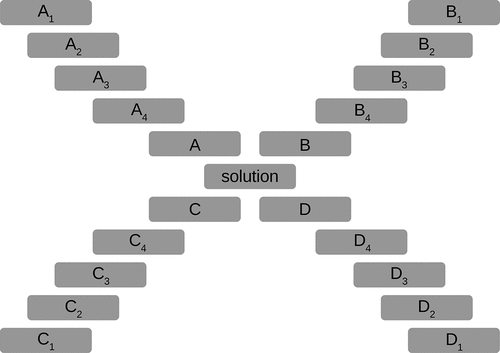
The goal of this experiment is to see how well a trained model can perform given this task. The original game plot is broken down into elementary puzzles for use in the model evaluation. In other words, a solution is sought based on four clues only. Final solution puzzles from the test set are considered equally to column puzzles.

Application of Natural Language Processing

This problem seems to be related to the field of distributional semantics. The idea of detecting associative words relies on the work of Miller and Charles (1991) that shows correlation of semantic similarity and contextual proximity in common text. Even though that work talks about words that have similar meaning and as such can substitute each other, a possibility of having a wider range of word relations is explored. Latest models produce word embedding mappings where every word is represented by an $N$-dimensional vector. These vectors are calculated using contextual information extracted from a training corpus. The context predicting models as described by Baroni, Dinu, and Kruszewski (2014) offer an improvement upon the older count-vector based approach.

A group of such models that even work in similar evaluation schemes outlined in the work of Mikolov et al. (2013a) are the so-called word2vec models. One flavor of this model is named continuous bag of words (CBOW), which works by averaging word vectors of context words on input, whereas the observed word is set on the output. The property of this approach is that the historical order of words does not affect the projections.

More interesting is the continuous skip-gram model that is used in this experiment. It works in the opposite way to CBOW by feeding an observed word as input and context as output. There exists a free and open-source implementation of this model in TensorFlow software library Abadi et al. (2015), which is slightly adapted here for the associations evaluation.

The Model

The previously mentioned word2vec is a well-documented and well-researched model for creating a word embedding space. The neural network for this model is a fairly simple one, as shown in Figure 2. It is a feed-forward class, with only one hidden layer. TensorFlow implementation accepts text only file as input for training. As a first training step, a vocabulary file is created containing all unique words from the text. This is then one-hot encoded as a vector of a size $V$, for use in training. During training, every word from the text is sequentially fed as input at each step, whereas its surrounding words are used on the output in process of unsupervised learning. A skip-gram window size is defined up front, to determine how large this surrounding is, hence defining the number of context words. Each context word is represented by a vector $Y_c$, where $c\in \{1,\dots ,C\}$. The window size is $C=2n$, where $n$ words precede the input word, and another $n$ follow it.

Figure 2. A block diagram of a skip-gram model where X represents the input vector. There is an embedding matrix $W$ that feeds the input vector to the hidden layer $H$, and an output weight matrix $W{ }^{\mathrm{\prime }}$. A sigmoid activation function is applied on the output layer $Y$ to scale the values on the $[0,1]$ interval.

As for the inner workings of the model, the hidden layer plays a major role. The size of the hidden layer, here denoted as $N$, defines the number of features that are expected to be detected in the training material. Choice of the number of features does affect the final result. During training, a sparse one-hot input vector is converted to an embedding matrix, of a size $V\times N$, which has dense properties. This is represented in Figure 3. These embedding represent vocabulary words in a kind of a hyper-sphere, an $N$-dimensional vector space. Namely, each input word represented as a vector $X_i$, where all values are set to zero except for the $i^{\mathrm{t}\mathrm{h}}$ value that is one, is transformed to a vector $E_i$ of a size $N$.

Figure 3. Illustration of a sparse to dense vector transformation. One-hot encoding of a word contains one at its corresponding index, and all other elements are zeros. When this is multiplied by the weight matrix $W$, resulting matrix contains embedding vectors consisting of only selected weights determined by the word index.

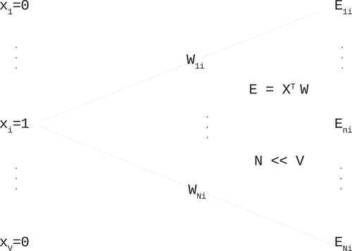
The hidden layer does not implement any activation functions, and the output vector is thus defined as

(1) $Y_c=W_c(X^{T}W).$(1)

The explanation of the training process is done with a reference to the work of Tixier, Vazirgiannis, and Hallowell (2016) similar to the experiment explained here. In each step, the error, which is detected on the output, gets propagated back through the network. Stochastic gradient descent method is used to adjust the weight values.

Presence of the softmax activation function on the output, turns the problem into a statistical analysis where a probability is calculated of having a particular context word, given a training word. As softmax normalizes input into a probability distribution, arbitrary input values get scaled to a $[0,1]$ interval. This is done by taking an exponent of an input value $y_{c,j}$, and averaging it over a sum of all input values. In this case, activation input values come from the output vector of the linear model $Y_c$.

(2) $p({\omega }_{c,j}={\omega }_{O,c}|{\omega }_I)=\frac{exp(y_{c,j})}{\sum _{j=1}^{V}exp(y_j)}$(2)

These type of models are also referred to as the log-linear models as in Gimpel and Smith (2010). Training of such models comes down to maximizing the probability given in Equation (2)(2) $p({\omega }_{c,j}={\omega }_{O,c}|{\omega }_I)=\frac{exp(y_{c,j})}{\sum _{j=1}^{V}exp(y_j)}$(2) . Overall likelihood is given as a product of context probabilities over the entire dictionary. Since there are $2n$ words in the context window, and there are $T$ words in the entire training set, this is given as:

(3) $\mathcal{L}=\prod _{t=1}^T\prod _{-n\le j\le n,j\ne 0}p({\omega }_{t+j}|{\omega }_t).$(3)

Final loss function is shaped by adding a negative sign for minimization, normalizing over the size of the training set, and adding a logarithm for numerical simplification.

(4) $J=-\frac{1}{T}\sum _{t=1}^T\sum _{-n\le j\le n,j\ne 0}logp({\omega }_{t+j}|{\omega }_t)$(4)

Evaluation

The original work of Mikolov, Yih, and Zweig (2013b) evaluates a trained model with the notion that words in a particular relationship have similar vector offsets. As an example, a relationship of a word “MAN” with a word “WOMAN,” would result in a similar embedding offset as “KING” and “QUEEN.” For an evaluation purpose, a target vector is calculated as a function of word vectors of two words in a relationship, and a third word that is in a similar relationship to the target as illustrated in Figure 4. The words used to compute the target are also referred to as analogies, and the computation is given by

(5) $T=C+(B-A).$(5)

Figure 4. Two-dimensional illustration of the original word2vec scenario. A target is computed using (5), and vocabulary words evaluated by their distances to the target.

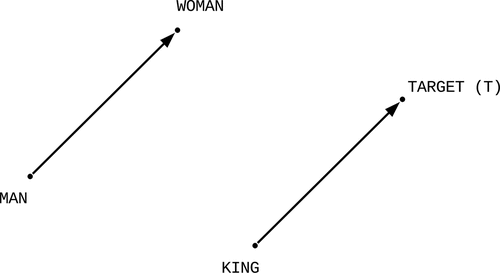
A vector of distances is then computed for all words in the vocabulary, using the target as a reference as in Mikolov, Yih, and Zweig (2013b). As the target is really just a guess, no word is most likely found at that particular position. The expected word is searched for in the distance vector in hope that it would come up among better rated results.

These distances are in fact cosine similarities, and for a random word $X$ and the target $T$, the similarity is calculated utilizing dot product as

(6) $cos(\mathrm{\angle }(X,T))=\frac{X\cdot T}{||X||||T||}.$(6)

For vectors that are the same, or most similar, this computes to $1$, and falling to $0$ for least similar (or orthogonal) words. The greater the similarity, the closer the word is to the target, hence it is said that the distance is smaller. In further text, the terms similarity and distance are used intermittently when discussing the results. During the evaluation process, similarities are sorted in a descending order, having the best word on top.

The previously described scenario is slightly modified for the associations application. In particular, a fourth analogy is introduced to account for four clues from the association game. The target is then computed by averaging these four clues as

(7) $T=\frac{1}{4}\sum _{i=1}^4{C}_i.$(7)

As in the original assessment, the vocabulary words are ordered based on their distances from the target $T$. An example of a nicely fit solution is given in Figure 5, but in practice there could be scenarios where analogies do not necessarily surround the solution. As the embedding space is an $N$-dimensional hyper-sphere, visualization of the vector distribution can only be an approximation and not very descriptive. Hence, two methods of rating are devised.

Figure 5. An example of a good fit, where the association solution “AIR” falls within the swarm of its corresponding analogies “ATMOSPHERE,” “LUNGS,” “BREATHING” and “OXYGEN.” There may still be a lot of other different words within the swarm spoiling the final result.

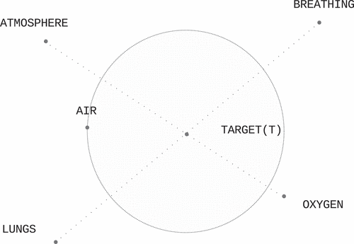
What is humanly most suggestive method, is the plain ordering of possible answers based on their distance from the target. This is how the quiz works, the puzzle is either solved or not. A player comes up with most probable possibilities and picks the best one. In the case of predicting an association, this is not always clear-cut. In the real game, people sometimes show very good ability this way, but on the other hand, a solution is not always found. In short, this rating is represented as the percentage of the evaluation scenarios that have predicted correctly within a certain number of words.

The other method is to show how well are the solution words clustered in contrast with the rest of the vocabulary. This is not very useful in solving the game but shows the capacity of the model to filter out the content and isolate word swarms in an associative way.

Training Set Preparation

Regarding the material used for training the previously described artificial neural network (ANN), there are quite a few obstacles that had to be worked around and could have had an impact on the final result. Some techniques are applied to overcome those problems and perhaps in this area future improvements might benefit more.

Major problem is that a professionally developed corpus for the Serbian language is not available. The material had to be assembled from any available resources, and that process is potentially problematic. There are no official electronic libraries. The only viable material that could be found was on the Internet. Great majority of written material, books, dictionaries and such come in a form of scanned texts with some method of the optical character recognition (OCR) processing applied. Most of these are found in a Portable Document Format (PDF), published along with pictures, references, footnotes and other publishing elements that affect text extraction. OCR applications introduce detection errors that are practically impossible to fix for large corpora. Material that is obtained in this form consists of dictionaries, common literature, manuals, text books and more.

The other form of source materials were news portals, various websites and the Serbian Wikipedia. Common property of these sources is that they typically tend to have correct spelling, and text extraction is somewhat more straightforward. This is due to the fact that these are purposely prepared and delivered in electronic form. There are however significant drawbacks as well.

News portals are frequently intermixed with, and reference foreign content. They also contain unusable forms like hashtags, web references and similar. There is also a problem due to utilization of various Serbian dialects that make the same word slightly different, thus unnecessarily increasing vocabulary size.

Another problem is the content extraction. Although articles are typically contained within identifiable HTML blocks, it is not always easy to extract just those. Usually other elements of a web page, like advertising, sidebars, navigation and similar, get in as well. The good side is that these do not intermix, and the original content block stays non compromised, meaning that its text flow is uninterrupted.

Other materials, like text books, literature and news portals, bring in volumes of data that get valuable contextual word relations into the model. However, to be able to effectively cover associative content, Serbian Wikipedia and dictionaries are of most benefit. Wikipedia is a massive library containing explanation of terms and constructs most people never heard of. Descriptive examples and content scenarios are frequently provided. Dictionaries, by the way they are usually written, artificially group related words like synonyms closer together and commonly provide sample text and explanations further enforcing contextual dependencies.

After assembling all sources, text extraction and merging together, the final training text was converted to lower case Cyrillic letters for its one to one character mapping. Single letter words, duplicate spaces, new line characters, no letter symbols and numbers were all removed. Presence of single letter words in the training text was very high due to various errors in text extraction. As single letter words also have high homonym affinity, it was decided to leave them out. The final word count of the training set came close to 300 million words. The vocabulary size for this text amounted to 1.7 million words.

As for the evaluation set, two different sources were used. One comes from a gaming website that offers association game, and the other are screenshots from the original TV program. The latter was OCR treated to produce usable data. This process also introduced detection errors, but due to its reasonably small size, was spell checked and manually corrected. This amounted to over 17 thousand unique test cases, each containing four clue phrases and a solution. As the model does not handle multiple word constructs, only puzzles with single word clues were considered, and those with single letter clues discarded. After comparing evaluation dictionary with the training vocabulary, more tests were discarded for not being represented in the training corpus. A total of 12 thousand cases were left for the experiment.

Vocabulary size of the training set standing at 1.7 million words, and as it influences the embedding matrix, proved not to be trainable, especially as it contains a lot of unusable words, errors, and similar. The idea of cleaning up such material effectively requires some form of spell checking and automatic error removal. The best spelling dictionary available was one from the LibreOffice software package. This one contains about 250 thousand words and also covers grammatical inflections a word can take in common text.

Although the number of words in the spelling dictionary looks initially substantial, after making a cross-reference with the evaluation vocabulary, it was proven not to be. It was discovered that not all words are present and the spelling dictionary is therefore insufficient. A few experiments were made with the training text cleaned up using different techniques, but in the end it was discovered that a simple process can be applied with very good results.

Final preparation used for the results presented here starts by identifying the testing vocabulary which is then used as a starting set. This is then compared with the spelling vocabulary. Words are extracted from the spelling vocabulary based on their similarities. This is done in order to pick up any possible grammatical modalities. Union of these two sets forms the final vocabulary that is then used to filter out the training corpus. Depending on the similarity factor, different results are presented, having different vocabulary sizes.

Results

As described previously, depending on the method of training set filtration, three different models were trained. This is done to compare different approaches in addition to finding the potential of the application. Training was performed using verbatim word2vec TensorFlow implementation with some additional fine tuning. Epoch evaluations were used as one of the criteria for stopping the training.

Original implementation uses a decreasing learning rate that starts with an initial value $0.2$. Once a stagnation of the learning progress is empirically determined, the training process is stopped and restarted with an arbitrarily smaller rate to make sure no further improvements can be achieved.

Evaluations during training were performed on the entire evaluation set, but only taking a score for the best $20$ words. This was done not only to speed up the training, but also to efficiently decide on the size (in number of neurons) of the hidden layer. Several models with hidden layer sizes ranging from $60$ to $160$ were evaluated, and it was determined that $120$ nodes is the optimal hyper parameter choice. Along with this modification, it was also found that the size of the skip-gram window that works the best is $[-6,6]$. Those results are presented here.

During training, model checkpoints were saved every ten minutes. Once model training was declared complete, evaluation sessions were performed on all saved checkpoints, but this time for the best one hundred words. This was done to allow for possible result variations to be picked up on a larger sample. Results are presented in two different ways.

The first scoring criterion measures the percentage of all evaluation cases that came up within one hundred best scoring words. The number one hundred was arbitrarily picked up as a subjective figure that seemed reasonable for practical purposes.

The second scoring criterion named stratification, evaluates the ability of the model to pick correct answers with the reference to the entire vocabulary. In other words, this would be the percentage of the vocabulary that contains solution words. It is obtained by taking the worst scoring word rank and calculated the percentage figure.

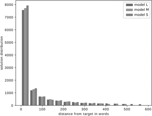
The results, just as described previously, are presented in Table 1. For better granularity of the model performance, a spread within the top one hundred words is broken down in ten equally sized bins and presented in Table 2. This is also provided in a form of a histogram for all three models in Figure 6, where the range of $600$ top words is broken down into $15$ evenly sized bins.

Table 1. Model parameters and evaluation results. Out of 12 thousand test cases, all projections fit within 600 best positioned words. Results are presented as a percentage of total vocabulary size, referred to as stratification, and as a percentage of scores within the best one hundred words against the total number of evaluations.

Model	Training corpus	Vocabulary size	Worst score	Stratification [%]	Score in 100 [%]
L	214549217	97563	591	0.6	76.68
M	200413189	65039	516	0.8	78.47
S	118100295	19336	392	2.0	81.12

Table 2. Number of correct solutions for each of the models and their corresponding distances from the target. This is presented for the top one hundred words broken down into ten equally sized bins.

Model	10	20	30	40	50	60	70	80	90	100	$\sum$
model L	4931	1369	772	549	403	300	277	212	197	192	9202
model M	5051	1456	750	515	410	340	287	231	184	193	9417
model S	5321	1346	781	528	461	364	291	237	215	191	9735

Figure 6. The histogram representation of the Table 2, only expanded to the best $600$ words.

Aside from the raw results, further analysis is performed to better understand the embedding space and the quality of each result. Because all three models displayed similar results, only model L is considered as it is created on the basis of the largest training set. Rather than extracting a visual representation of the embedding hyper-sphere, we look into the distances matrix and the word swarms around targets.

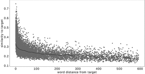
The first analysis is presented in Figure 7 and represents cosine similarity scores against solution word distances from their corresponding targets. This is done to see what part the similarity factor plays in guessing the correct word. Each dot represents a similarity of a solution for the corresponding word distance from its target. For better assessment, a moving average graph overlay is included. It can be observed that words with higher ranks have somewhat higher similarity factors. This increase is pronounced for the first one hundred words, but then slightly falls off. As the similarity factor is a measure of how close the words are, this trend is expected although not very pronounced.

Figure 7. Cosine similarity values between target points and the corresponding solutions over their rank positions within the descending similarity vectors for the model L. Value of $1$ would refer to the most similar, actually identical word, while $0$ is the least similar.

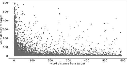
The second assessment, given in Figure 8, is looking into a swarm density around target words. Each dot represents the number of words that have cosine similarity score higher than $0.3$. This graph somewhat correlates with the distance graph, although pretty high densities are observed for poorly scoring words as well.

Figure 8. Word density defined as the number of words with cosine similarity higher than $0.3$ that are found around the target word. Each point represents the density for a puzzle with the solution found at a particular rank, as extracted from the model L.

As a final check, a list of best scoring words is printed out for manual inspection. This result is impossible to present here since there is no numeric quality to it, but the observation is quite telling. Essentially, all words that were looked at, contain such a striking associative relation to the solution word that any of them could easily be substituted by any of the puzzle words with no impact to validity of the game.

Conclusions

With this latest revelation, it seems the most viable result that can be reported is the model stratification factor mentioned and defined earlier. This figure of merit is really painting the picture about the ability of the model to separate quality answers from the so-called noise. This number for obvious reasons gets better with larger training sets as reported in Table 1. Although one would expect a model to produce perfect answers, for this particular application the number of possible correct answers is quite large and hence difficult to guess correctly in a small number of attempts.

Best assessment of the model would be to compare its performance against a real life human counterparts. In theory, this is possible although small modifications would be required. As the model assesses only the cases where all four clues are known, this would have to be expanded to cover the cases with fewer clues. The reason is that people tend to occasionally make correct guesses even after having only one word known. For a complete comparison, all possibilities must be included. Only this way, a proper performance evaluation could be made. If it could be proven that humans fare better in certain or all cases, perhaps a second stage of the model could be devised that works by refining the output words in some way.

The main problem in making this real life evaluation comes from the fact that no statistical data from the original TV show exists, or it is at least publicly unavailable to the best of authors’ knowledge. There are only recorded TV programs, but as those are in their thousands, a laborious manual process would have to be undertaken to shape them in a usable form.

Although a result of about $80\mathrm{\%}$ of correct guesses within the best one hundred words seems decent, only about $40\mathrm{\%}$ are really useful in a real game scenario. This is the number of correct answers in the first ten words. As there is a limited number of guesses allowed which are enforced by strict time limit, $40\mathrm{\%}$ is perhaps a true measure of success this model would have in a real game.

Rather than solving a game, there is perhaps a much better application for a model such as this one. The proven ability of the model to cluster the training corpus to $2\mathrm{\%}$ or less can be applied to construct the association puzzles. A person creating a game could perhaps input just one word into the model and get a decent range of possibilities to complete each puzzle. Such models can be trained on data sets filtered exclusively on well rounded spelling dictionaries and therefore contain rather large vocabularies. One point of model training time and size optimization could be to exclude grammatical inflections by substituting all different forms of a word with one representative.

Disclosure Statement

No potential conflict of interest was reported by the author(s).

References

- Abadi, M., A. Agarwal, P. Barham, E. Brevdo, Z. Chen, C. Citro, G. Corrado, A. Davis, J. Dean, M. Devin, et al. 2015. TensorFlow: Large-scale machine learning on heterogeneous distributed systems.
- Baroni, M., G. Dinu, and G. Kruszewski. 2014. Don’t count, predict! a systematic comparison of context-counting vs. context-predicting semantic vectors. 52nd Annual Meeting of the Association for Computational Linguistics, ACL 2014 - Proceedings of the Conference 1:238–2288.
- Gimpel, K., and N. A. Smith 2010. Softmax-margin CRFs: Training log-linear models with cost functions. In Proceedings of the 2010 Annual Conference of the North American Chapter of the Association for Computational Linguistics: Human Language Technologies (NAACL HLT 2010), 733–36. Los Angeles, CA: Association for Computational Linguistics.
- Mikolov, T., K. Chen, G. Corrado, and J. Dean 2013a. Efficient estimation of word representations in vector space.
- Mikolov, T., W.-T. Yih, and G. Zweig 2013b. Linguistic regularities in continuous space word representations. In Proceedings of the 2013 Annual Conference of the North American Chapter of the Association for Computational Linguistics: Human Language Technologies (NAACL HLT 2013), Atlanta, Georgia, 746–751.
- Miller, G. A., and W. G. Charles. 1991. Contextual correlates of semantic similarity. Language and Cognitive Processes 6 (1):1–28. doi:10.1080/01690969108406936.
- Tixier, A. J., M. Vazirgiannis, and M. R. Hallowell 2016. Word embeddings for the construction domain. CoRR, abs/1610.09333.