An Artificial Intelligence Neural Network Predictive Model for Anomaly Detection and Monitoring of Wind Turbines Using SCADA Data

ABSTRACT

The industry 4.0 has created a paradigm shift in how industrial equipment could be monitored and diagnosed with the help of emerging technologies such as artificial intelligence (AI). AI-driven troubleshooting tools play an important role in high-efficacy diagnosis and monitoring processes, especially for systems consisting of several components including wind turbines (WTs). The utilization of such approaches not only reduces the troubleshooting and diagnosis time but also enables fault prevention by predicting the behavior of different components and calculating the probability of near future failure. This not only decreases the costs of repair by providing constant component’s monitoring and identifying faults’ causes but also increases the efficacy of the apparatus by lowering the downtimes due to the AI-driven early warning system. This article evaluated, compared, and contrasted eight different artificial neural network (ANN) models for diagnosis and monitoring of WTs that predict the machinery’s system failure based on internal components’ sensor signals and generation temperature. This article employed a machine learning model approach with two hidden layers using multilayer linear regression to achieve its objective. The developed system predicted the output of the WT’s generator temperature with an accuracy of 99.8% with 2 months in advance measurement prediction.

Introduction

Industry 4.0 introduced a new paradigm to the machineries’ monitoring and diagnosis procedure. Enabled by advances in artificial intelligence (AI) and notions such as Internet of Things (IoT) in recent years, Industry 4.0 has proved to be an effective and reliable trend toward digitization and automation (Haag and Anderl 2018). Industry 4.0 is the fourth paradigm shift and major breakthrough in industrial revolution made possible by the advancements in electronics and information technology; a continuation of the evolution of automation commenced from the invention of steam engines and mass production as a result of assembly lines and standardization (Xu, Xu, and Li 2018).

The wind power industry and the whole renewable energy sector could benefit significantly from the employment of industry 4.0. Most of the machineries including wind turbines (WTs) produce a huge amount of data related to power consumption, current, voltage, vibration, and environmental factors that are not necessarily utilized. The information processed from these gathered data could be used to improve the troubleshooting, monitoring, and maintenance procedures. Sensors attached to different parts of WTs will provide important data of the health state of the apparatus, which require interpretation and processing.

With the advancement of sensor technology and IoT systems, new types of smart sensors have been developed and employed for data collection purposes in WTs, which laid the foundation for ML-based performance improvement, condition monitoring, and fault prediction applications (Aitken et al. 2014; Hang, Zhang, and Cheng 2014; Mieloszyk and Ostachowicz 2017).

There have been several studies toward the use of data gathered from WTs’ embedded sensors to improve the performance, implement condition monitoring (CM) and defect prediction and identification, and to analyze and evaluate the behavior of WTs (Eroglu and Seçkiner 2019; Nithya, Nagarajan, and Navaseelan 2018; Yuan, Sun, and Ma 2019; Zhang et al. 2014).

For example, in Germer, Kleidon, and Leahy 2019, an estimation of ideal monthly wind energy generation of WTs’ air density and wind speed from database-gathered data from WTs in Germany between 2000 and 2014 was compared against the actual yield. Based on the statistical analysis, the turbine age and park size had a significant effect on the reduction of the overall yield. The cross-examination between the estimation and the actual yield confirmed a high accuracy estimation. Nonetheless, the actual monthly yield proved to have 73.7% of the ideal yield, the cause of which was not identified. The research concluded that the prediction based on the wind energy generation was a reliable method to derive realistic estimation. In another attempt, Nachimuthu et al. (Nachimuthu, Zuo, and Ding 2019) developed a decision-making model for maintenance optimization of offshore WTs by taking into account the uncertainties and unknown factors. The research has developed a mathematical model to facilitate the decision-making process for wind farm stakeholders. A four-category failure classification was developed each with a corresponding maintenance rank. Based on that, the developed model managed to estimate the probability of each failure. The team aims to incorporate other factors including lead-time, logistic time, weather, sea-state condition, and the hydrodynamics of the sea in their future development of the mathematical and decision-making model. Moreover, Yang et al. (Yang and Sørensen 2019), presented a Markov chain model to investigate and predict a six-level damage categorization scheme for WTs’ blades. The aim of the research was to provide a cost-optimal inspection facility and maintenance strategy for WTs. A statistical damage evolution of WTs’ blades simulation was developed based on the calibrated transition probabilities in the discrete Markov chain model. Additionally, a condition-based maintenance strategy and the classical Bayesian pre-posterior decision theory were implemented for decision-making.

In Shihavuddin et al. (Shihavuddin et al. 2019), a faster R-CNN deep learning model was developed to assess images captured by an inspection drone for automatic damage analysis in WT blades. Four different classes were defined and manually annotated for the supervised deal learning model including Leading Edge erosion, Vortex Generator panel, and Vortex Generator with Missing Teeth and Lightning Receptor. Overall, 305 labels were annotated for the training data set and 173 for testing. The research concluded a robust detection system with a very high accuracy for WT blade damage inspection.

In Saenz-Aguirre et al. 2019, a neural network-based model to control active gurney flap flow with the aim of enhancing the aerodynamic adaption capability of the TWs was developed. The flow control system was designed to achieve an optimal operation according to the fast variations of the weather. The wind speed data obtained from the meteorological station were used for Blade element momentum (BEM)-based calculations to analyze the aerodynamic behavior of WT’s blades, while the aerodynamic data calculated by computational fluid dynamics (CFD) were fed to the developed artificial neural network (ANN) model.

In the study by Qian et al. (Qian, Ma, and Zhang 2017), an online sequential extreme learning machine (OS-ELM) algorithm was developed to estimate the heath condition of WTs' drivetrain systems. A physical kinetic energy correction model was utilized in order to normalize the temperature changes at the rated power output in order to eliminate the effect of speed variation of the WTs. It was concluded that the proposed method has higher efficiency for both the long-term aging characteristics and the short-term faults of the gearbox. Additionally, Amini et al. (Amini, Kanfound, and Gan 2019) proposed an ANN algorithm based on the single hidden-layer feed forward neural network (SLFN) and gradient-based backpropagation (BP) training to monitor the health condition of a WT generator. The researchers used data gathered from six sensors with eight channels including two single axis-accelerometer, one triaxial accelerometer, one acoustics (microphone), one temperature, and one light sensors (for rotational speed) with a sampling data collection rate of 51.2 kHz to predict the WT’s bearing health condition and represent it in the real-time dynamic 3-D digital twin model. The developed model achieved an accuracy of 83.33% in the vibration-based CM prediction across the three different rotation speed of 15 Hz, 9 Hz, and 12 Hz.

In the study by Canizo et al. (Canizo et al. 2017), a cloud-based predictive maintenance model was developed for failure prediction of WTs comprising three main modules including a predictive model for each WT based on the Random Forest algorithm, a monitoring agent providing failure prediction in 10 minutes intervals for the next hour of data collection, and a GUI interface to visualize the information obtained from the developed model. The research improved upon previous attempts in terms of scalability, automation, and data processing speed and at the same time providing a centralized access point to gather and analyze all the data received from WTs, reducing the operation and maintenance costs.

Furthermore, in Kusiak and Verma 2012, data gathered from on-site sensors embedded in 24 WTs were used to develop a method for analysis of different bearing faults. The research proposed a data mining algorithm to train and test the evaluation results deployed in three different ANN models optimized to collect the information about the relationship between the WTs’ generator bearing temperature and input parameters under the normal condition. The research resulted in the identification of the bearings’ faults, the main affecting factors that can be utilized for CM and WTs’ bearing behavior prediction purposes.

This research explored and evaluated the deployment of three different ANN algorithms for diagnosis and monitoring of WTs to predict the WT’s system failure based on its internal components’ sensor signals and generation temperature. The algorithm used the historic supervisory control and data acquisition (SCADA) data collected from nine WTs over 10 years received from the Westmill Windfarm located in Swindon, United Kingdom.

Methods

Around 12 GB of SCADA data recording of nine WTs over a ten-year period were acquired at a sampling frequency of ~0.0016 Hz for this experiment. The recording frequency was 10 minutes including each sensor node’s alarm data. Five initial ML models were developed as preliminary analysis for WTs’ generator temperature prediction. Figure 1 shows the flowchart of the inputs and output of the developed temperature ML models with several different inputs.

Figure 1. The flowchart of the inputs and output of the developed temperature models with several different inputs.

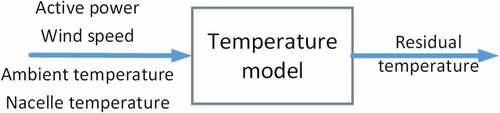
Five ML models were initially developed to compare and contrast their performance with different WT sensors’ data configuration as their inputs as is shown in Table 1.

Table 1. The different sensors’ data input configuration for the five ML models

The output of all five ML models is ”Generator temperature,” with models 1, 3, 4, and 5 each having a single temperature for its input, while Model 1 has standard deviations for ambient temperature, active wind speed, and active power in addition to its mean values as the input. For Model 2, we decided to include all three temperatures including ambient, external, and internal temperatures as the input. All models feature the mean values for active wind speed and active power as their inputs. The configuration of the different ML models’ inputs was designed to select the optimal input data for the final, most accurate model. Inputs of Models 2, 3, 4, and 5 were defined to observe the impact of the inclusion configuration of different temperature sensors on the efficacy of the output ML model, while Models 1 and 3 were designed to explore the accuracy improvement of inclusion of standard deviation values for each input.

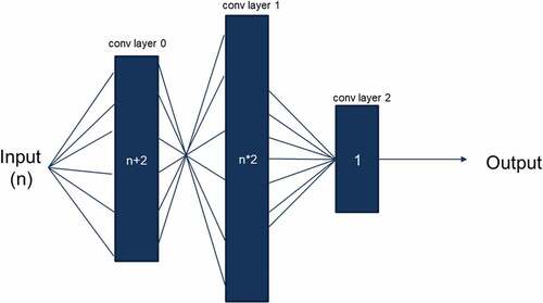
A fully connected ANN model was developed with two hidden layers as Figure 2 depicts. The ML model has a dynamic structure in which the ‘conv layer 0’ numbers of nodes vary depending on the model’s inputs. The model adds two nodes to the number of that model’s sensor’s data inputs. Moreover, “conv layer 1” multiplied the number of model’s inputs by a factor of two and feed the data to the output layer (conv layer 2).

Figure 2. The schematic layout of the ML regression algorithm.

The ML models were developed using TensorFlow and Keras backend with the batch size of 100 per epoch and a training epoch of 50,000. The training data set was chosen from one WT for the period of 1 year from 01/01/2017 to 31/12/2017, whereas the validation data set period was from 01/01/2018 to 30/05/2018 (200 K data entries) including 1 known incident commenced on 14/02/2018. These timeframes were chosen to develop ML models based on healthy conditions and then use them for fault diagnosis and prediction. If the predicted generator temperature deviates with a statistically significant value from the actual values, one could infer that a failure has commenced. The training data set time slot was carefully chosen to be free of any known incidents that might affect the ML models’ accuracy negatively. For the testing data set, a 10% section of the training data set was randomly allocated for all the models. The ML models showed a similar result in terms of accuracy for minimum, maximum, and standard deviation error offset value. Table 2 shows the comparison between the five developed ML models in which “Model 2” proved to have the highest statistically significance accuracy among the rest of the models followed by Model 1.

Table 2. Models’ accuracy for minimum, maximum, and standard deviation offsets between the predicted and actual recorded values

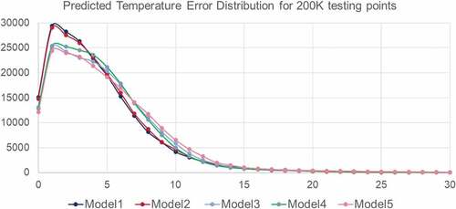
Figure 3 depicts the predicted generator’s temperature error distribution obtained from five MLs based on the testing data set. The horizontal axis represents the error offset value, while the vertical axis shows the frequency of their occurrences.

Figure 3. Models’ predicted generation temperature absolute error distribution based on the testing data set.

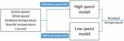
The results from Table 2 and Figure 3 led to the development of the hypothesis in which the inclusion of all three temperatures including ambient, internal, and external as well as the standard deviation values for each sensor’s data as the model input data would help increasing the overall ML model accuracy. Thus, further three ML models were developed with all three temperatures as their inputs including their standard deviation values as the basis and other sensory data to explore the possibility of increasing the model’s accuracy and lowering the error offset values for both maximum and standard deviation even more. One of the key factors, which was added to the new model sets, was the inclusion of the generator shaft speed, which results in different current values. Thus, for each of the three new ML models, two submodels were developed, one for high shaft speed and the other for low shaft speed in order to increase the overall accuracy of the ML models based on the current condition of the WTs. The original data for both training and testing were consequently filtered to split the data into two submodels for both high and low shaft speeds. As Figure 4 depicts, for low shaft speed, the speed bracket was chosen between 995 and 1005 rpm, and similarly, for high shaft speed, a bracket of speed between 1495 and 1505 rpm was selected. Any values outside these two thresholds were omitted from the training data set for both submodels.

Figure 4. The flowchart of the inputs and output of the new temperature models including submodels for high and low shaft speeds.

Table 3 shows the three ML models derived from the results derived from original Models 1 and 2 configurations including their input data. As discussed before, all the three new models comprised all temperature data including their standard deviation values. Moreover, new Models 2 and 3 have shaft speed (current) data as shown in Table 3. In addition to the shaft speed, Model 3 also comprised historical data of the generator temperature, i.e., the previous output values were used as one of its inputs up to three consecutive timestamps. The reason for this was to check whether including previous generator temperature data as an input for the current time would have a statistically significance impact on the accuracy of the prediction model.

Table 3. The different sensors’ data input configuration for the three ML models for both submodels of high and low shaft speeds

Results

The new three ML models (six including both low and high rpm models) used the same training and testing data sets with the same hyperparameters as the initial five ML models. The results (Table 4) showed a significant improvement over the initial models’ configurations. Model 3 with historical data as its input showed the lowest error in all settings, i.e., mean and standard deviation errors for both its submodels including high and low shaft speed in the overall test data set.

Table 4. Models’ accuracy for the mean and standard deviation offsets between the predicted and actual recorded values for both submodels of high and low shaft speeds

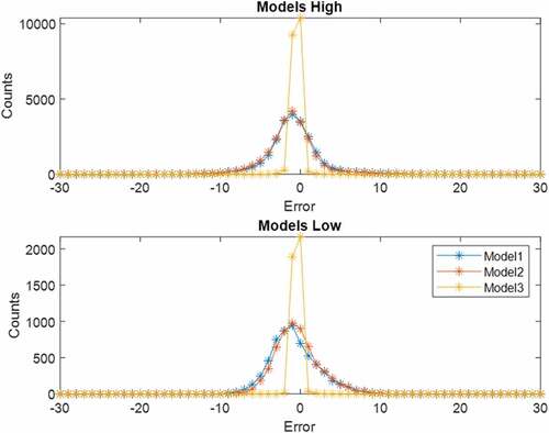
Nonetheless, although the Model 3 prediction of the generator’s temperature was very close to the actual recorded value, it failed to predict the actual failure in the testing data set, and during the incident period, its prediction accuracy was proven to be the worst among the rest of the models. Figure 5 shows the real error distribution among the three ML models. As it can be seen from Figure 5, Model 3 has the lowest real error values between the predicted and real generator temperature values, but it failed once a generator incident happened for both its high and low submodels possibly from overfitting issues. One could hypothesize that adding historical generator’s temperature as one of the model’s inputs could lead to generalization error due to overfitting. As a result, the second to the best model (Model 2) was chosen as the best predictor models from the list in Figure 5.

Figure 5. Models’ predicted generation temperature real error distribution based on the testing data set for both submodels of high and low shaft speeds.

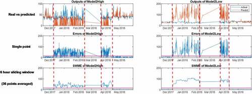
As mentioned before, Model 2 has the best overall prediction accuracy among the rest of the models and could predict the WT’s generator temperature with the lowest error offset to the actual recorded values. Figure 6 shows the performance of Model 2 for both its submodels (high and low rpms) in the training data set time duration with no defects or failures, whereas Figure 6 shows the performance of the model in the testing data set time duration including the one known generator failure commenced on 14/02/2018. As the “real vs predicted” and “single point” sections of the figure show, the model successfully predicted the generator’s failure including the temperature issues leading to the failure, starting from mid-January 2018, Figures 6 and 7.

Figure 6. The performance of the model in the training data set time duration including single point and 6 hours sliding window results for both submodels of high and low shaft speeds.

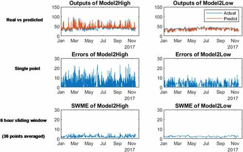
Figure 7. The performance of the model in the testing data set time duration including single point and 6 hours sliding window results for both submodels of high and low shaft speeds.

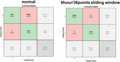
Error! Reference source not found. illustrates the confusion matrix for Model 2 in both normal and 6 hours/36 points sliding window modes. The normal confusion matrix did not yield a very high accuracy as it can be seen from the graph. It reported a 37% overall accuracy among its true-positive and true-negative prediction. However, the 6 hour/36points sliding, on the other hand, proved to have a higher statistically significant accuracy (99.8% both among its true-positive and true-negative prediction), Figure 8.

Figure 8. The overall Model 2 confusion matrix both in normal and 6 hour/36 points sliding.

Discussion

Three ML models were derived from the initial five ML models as it was concluded that the inclusion of internal, external, and ambient temperatures as well as the addition of standard deviation values of all the sensor’s data inputs has a statistically significant improvement effect on the models’ prediction accuracy. The inclusion of historical generator temperature although yielded the lowest error offset between the prediction and the actual recorded generator’s temperature failed in predicting the system failure possibly due to generalization errors caused by overfitting. For the three models derived from the initial five models, two submodels for both high and low generator’s shaft speeds were developed to increase the accuracy of the models even further. These two submodels are transparent to the operator and are triggered upon the detection of the generator’s shaft speed analysis based on the current WT’s condition. Among all the developed models, Model 2 was concluded to be the best fit for the use case WTs’ data set. The 6 hours/36 points sliding window confusion matrix for the top performing model (Model 2) showed a promising result in the WTs’ generator temperature for both predicting true positives and true negatives as well as dismissing false-positive and false-negative values. A thresholding system has also been implemented, so an operator would get a notification about a possible failure in advance and would have enough time to act accordingly. It was concluded that the regression models developed based on temperature of the generator allow us to detect a defect developing around two months before the WT’s shutdown.

Conclusion

Eight different ML models were developed with different sensors’ data based on SCADA data collected from nine WTs over 10 years received from the Westmill Windfarm located in Swindon, United Kingdom, to predict the generator failure in WTs in advance using pattern recognition based on historical data. The results of each model’s accuracy in terms of minimum, maximum, and standard deviation offsets between the predicted and actual generator temperature values were compared and contrasted, and the effect of the input sensor data was explored. Overall, this research showed the possibility of utilizing ML-driven regression algorithms to predict WTs’ generator failure caused by heat, lowering the maintenance costs related to downtime and staff,and, at the same time, improving the operational availability of the apparatuses. For the future works, the authors of this article aim to explore the possibility of implementing transfer learning for fast adaptation and deployment of the trained models to new WTs, allowing quick training of new assets and lowering the readiness time required for the model.

Disclosure Statement

No potential conflict of interest was reported by the author(s).

References

- Aitken, M. L., R. M. Banta, Y. L. Pichugina, and J. K. Lundquist. 2014. Quantifying Wind Turbine Wake Characteristics from Scanning Remote Sensor Data. Journal of Atmospheric and Oceanic Technology 31 (4):765–880. doi:10.1175/JTECH-D-13-00104.1.
- Amini, A., J. Kanfound, and T. H. Gan. 2019. An Ai Driven Real-Time 3-D Representation of an off-Shore WT for Fault Diagnosis and Monitoring. ACM International Conference Proceeding Series, Istanbul, Turkey. pp. 162–65.
- Canizo, M., E. Onieva, A. Conde, S. Charramendieta, and S. Trujillo. 2017. Real-Time Predictive Maintenance for Wind Turbines Using Big Data Frameworks. 2017 IEEE International Conference on Prognostics and Health Management, ICPHM, Dallas, TX, USA. pp. 70–77.
- Eroglu, Y., and S. U. Seçkiner. 2019. Early Fault Prediction of a Wind Turbine Using a Novel ANN Training Algorithm Based on Ant Colony Optimization. Journal of Energy Systems 3 (4):139–47.
- Germer, S., A. Kleidon, and P. Leahy. 2019. Have Wind Turbines in Germany Generated Electricity as Would Be Expected from the Prevailing Wind Conditions in 2000-2014? PLoS ONE 14 (2):1–16. doi:10.1371/journal.pone.0211028.
- Haag, S., and R. Anderl. 2018. Digital Twin – Proof of Concept. Manufacturing Letters 15:64–66. doi:10.1016/j.mfglet.2018.02.006.
- Hang, J., J. Zhang, and M. Cheng. 2014. Fault Diagnosis of Wind Turbine Based on Multisensors Information Fusion Technology. IET Renewable Power Generation 8 (3):289–98. doi:10.1049/iet-rpg.2013.0123.
- Kusiak, A., and A. Verma. 2012. Analyzing Bearing Faults in Wind Turbines: A Data-Mining Approach. Renewable Energy 48:110–16. doi:10.1016/j.renene.2012.04.020.
- Mieloszyk, M., and W. Ostachowicz. 2017. An Application of Structural Health Monitoring System Based on FBG Sensors to Offshore Wind Turbine Support Structure Model. Marine Structures 51:65–86. doi:10.1016/j.marstruc.2016.10.006.
- Nachimuthu, S., M. J. Zuo, and Y. Ding. 2019. A Decision-Making Model for Corrective Maintenance of Offshore Wind Turbines Considering Uncertainties. Energies 12 (8):1408. doi:10.3390/en12081408.
- Nithya, M., S. Nagarajan, and P. Navaseelan. 2018. Fault Detection of Wind Turbine System Using Neural Networks. Proceedings - 2017 IEEE Technological Innovations in ICT for Agriculture and Rural Development, TIAR 2017 2018-Janua, Chennai, India. pp. 103–08.
- Qian, P., X. Ma, and D. Zhang. 2017. Estimating Health Condition of the Wind Turbine Drivetrain System. Energies 10 (10):1583. doi:10.3390/en10101583.
- Saenz-Aguirre, A., U. Fernandez-Gamiz, E. Zulueta, A. Ulazia, and J. Martinez-Rico. 2019. Optimal Wind Turbine Operation by Artificial Neural Network-Based Active Gurney Flap Flow Control. Sustainability (Switzerland) 11 (10):2809.
- Shihavuddin, A. S. M., X. Chen, V. Fedorov, A. N. Christensen, N. A. B. Riis, K. Branner, A. B. Dahl, and R. R. Paulsen. 2019. Wind Turbine Surface Damage Detection by Deep Learning Aided Drone Inspection Analysis. Energies 12 (4):1–15. doi:10.3390/en12040676.
- Xu, L. D., E. L. Xu, and L. Li. 2018. Industry 4.0: State of the Art and Future Trends. International Journal of Production Research 56 (8):2941–62. doi:10.1080/00207543.2018.1444806.
- Yang, Y., and J. D. Sørensen. 2019. Cost-Optimal Maintenance Planning for Defects on Wind Turbine Blades. Energies 12 (6):998.
- Yuan, T., Z. Sun, and S. Ma. 2019. Gearbox Fault Prediction of Wind Turbines Based on a Stacking Model and Change-Point Detection. Energies 12 (22):4224. doi:10.3390/en12224224.
- Zhang, C., F. M. Zhang, F. Li, and H. S. Wu. 2014. Improved Artificial Fish Swarm Algorithm. Proceedings of the 2014 9th IEEE Conference on Industrial Electronics and Applications, ICIEA, Hangzhou, China. pp. 748–53.