Using Skeleton Correction to Improve Flash Lidar-based Gait Recognition

ABSTRACT

This paper presents GlidarPoly, an efficacious pipeline of 3D gait recognition for flash lidar data based on pose estimation and robust correction of erroneous and missing joint measurements. A flash lidar can provide new opportunities for gait recognition through a fast acquisition of depth and intensity data over an extended range of distance. However, the flash lidar data are plagued by artifacts, outliers, noise, and sometimes missing measurements, which negatively affects the performance of existing analytics solutions. We present a filtering mechanism that corrects noisy and missing skeleton joint measurements to improve gait recognition. Furthermore, robust statistics are integrated with conventional feature moments to encode the dynamics of the motion. As a comparison, length-based and vector-based features extracted from the noisy skeletons are investigated for outlier removal. Experimental results illustrate the superiority of the proposed methodology in improving gait recognition given noisy, low-resolution flash lidar data.

Introduction

The problem of gait identification has received significant interest in the last decade due to the various applications in areas ranging from intelligent security surveillance and identifying persons of interest in criminal cases to designated smart environments (Charalambous 2014; Jain, Bolle, and Pankanti 2006). Gait analysis also plays an important role in quantifying the severity of certain motion-related diseases such as Parkinson’s disease (Din, Silvia, and Rochester 2016). While the iris (Daugman 2009), face (Schroff, Kalenichenko, and Philbin 2015), and fingerprint (Maltoni et al. 2009) provide some of the most robust biometrics for person identification, they require the cooperation of subjects as well as the availability of high-quality data. However, many scenarios exist in which the subjects cannot be controlled or acquisition of data is impossible. Under such circumstances, biometrics that can be extracted from gait have shown promising results in several studies (Preis et al. 2012; Sinha, Chakravarty, and Bhowmick 2013). Features extracted from gait are resilient to changes in clothing or lighting conditions compared to color or texture, which are among the prevalent features for person identification. While patterns of walking may not be necessarily unique to individuals in practice, a combination of biometric-based static attributes, along with motion analysis of certain body joints, can create an effective set of features to recognize an individual.

Video-based gait recognition approaches are generally divided into two main categories, model-based, and model-free methods. Model-free methods rely on features that can be obtained from clean silhouettes. Fitting a model, such as a skeleton to human silhouettes, and using the extracted features from such a model for gait recognition is categorized as a model-based approach. The model provides benefits in terms of data compaction, computation, storage, scalability, and recognition accuracy. Furthermore, the skeleton-related attributes mimic actual physical traits in the human body and can be utilized as a soft biometric.

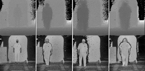
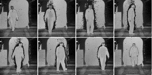
In recent years, depth cameras have become popular for gait analysis mainly due to their ability to provide a three-dimensional depiction of the scene (Batabyal, Vaccari, and Acton 2015; Clark et al. 2013; Sadeghzadehyazdi, Batabyal, and Acton 2021). Unlike their optical counterparts, depth cameras, such as lidar and Kinect, can provide depth information that is not sensitive to lighting conditions. In this work, we utilize flash lidar to collect data. A flash lidar camera uses a pulsed laser to illuminate the whole scene and simultaneously record depth (range) and intensity information. Figure 1 shows example frames of the intensity and depth data collected by a flash lidar camera.

Figure 1. Sample frames of lidar data. The top and bottom rows show depth (range) and intensity data, respectively.

With a limited number of studies, the only existing lidar-based person identification works are model-free and rely on background subtraction to extract human silhouette from the point cloud data provided by Velodyne’s rotating multi-beam (RMB) lidar system (Benedek et al. 2018; Gálai and Benedek 2015). In general, pose estimation using point cloud data can be a computationally expensive problem (Xuequan et al. 2018, 2019; Zhao et al. 2021).

Existing model-based methods take advantage of high-quality skeleton data provided by Kinect or mocap and avoid the challenge of erroneous features. However, as we will discuss in TigerCub 3D flash lidar, these modalities are not always a proper choice for real-world applications. In contrast to Kinect and mocap, flash lidar has shown successful applications in numerous real-world applications. However, unlike Kinect and Mocap, the data collected by a flash lidar camera are noisy and have a low resolution that limits the performance of skeleton extraction systems. Features that are computed from the spurious skeleton models are likewise erroneous, which presents a major challenge to a successful gait recognition. Under the described conditions, a common approach is to remove low quality and missing data, and then to perform the gait analysis on the remaining higher-quality information. The work described in this paper takes an alternative approach by presenting a filtering mechanism to correct erroneous and missing skeleton joints. The correction mechanism is valuable because the original data, which is costly to collect, can be preserved. In addition, we won’t lose temporal information that encodes the dynamics of the motion.

The proposed design contributes to improving gait recognition using flash lidar data, with three main contributions:

1. We present a filtering mechanism that exploits polynomial interpolation and robust weighted regression to correct for noisy and missing measurements of joint coordinates that results in data preservation.

2. With extensive skeleton correction, we show that traditional feature moments can serve as a better representative of motion dynamics if they are considered along with robust statistics for outlier identification.

3. As an alternative method for applications where data elimination is not an issue, we investigate features extracted from noisy skeletons for outliers, and present a method for detecting outliers in vector-based features.

It is important to note that our work is not intended to introduce a complex methodology for the gait recognition problem in general. Instead, we aim to present an efficient pipeline for gait recognition for flash lidar data without data removal. This is a challenging problem with its own complexities, due to the low-quality and noisy lidar data.

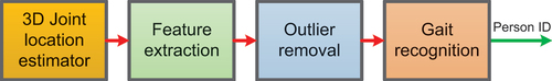
In this work, we take a model-based approach, leveraging OpenPose, a pre-trained deep network (Cao et al. 2017), to extract a skeleton model from the intensity information. Using camera properties and the depth data, the skeleton joint coordinates can be transformed into real-world coordinates. By modeling the coordinates of each joint through time as a set of time sequences, we use Tukey’s test (Tukey 1977) for an automated outlier removal, and present a method for detecting outliers in vector-based features. To address data elimination and loss of temporal information as a result of outlier removal, we present GlidarPoly (gait recognition by lidar through polynomial correction), a filtering mechanism that corrects erroneous skeleton joints and recovers the missing joint data, instead of eradicating them. We also integrate robust statistics to the conventional feature moments to capture motion dynamics and improve gait identification after correction of the skeleton joints. Figures 3 and 4 show the pipeline of joint correction and outlier removal methodologies, respectively.

The remainder of this paper is organized as follows. First, the related works are presented in the subsequent section. Next, the proposed methodology is presented, followed by results and discussion. We finish the paper with a conclusion section.

Related Works

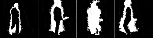
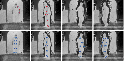
In our dataset, recorded by a single flash lidar camera, several factors diminish the quality of features that are computed from the resulting joint positions. As the subjects proceed toward the camera, depth data are affected by noise. The lack of color in the intensity data and the similarity between human clothing, background, and skin are some of the other elements that can negatively affect the quality of segmented silhouettes, detected poses, and consequently the feature vectors. Figure 2 shows examples of faulty detected silhouettes. There are a large number of frames with no detected silhouette, mostly in successive frames. This loss of data occurs when a subject is farther from the camera and close to the background, or when there is minimal movement.

Figure 2. Examples of noisy segmented silhouettes from flash lidar data.

There are a few studies in the literature that address the problem of gait identification under low quality or missing silhouette conditions. Iwashita, Uchino, and Kurazume (2013) and Tang et al. (2016) consider cases with incomplete silhouettes, but do not consider the cases when an entire silhouette is missing. In general, these studies depend on the reference silhouettes being correctly segmented. Silhouette reconstruction methods such as inpainting are only effective when smaller parts of the silhouette are missing (Tang et al. 2016). Methods based on gait features such as gait energy image (GEI) (Han and Bhanu 2005) and its variations, that are less sensitive to segmentation error, are also based on the non-missing silhouette criterion. While in Babaee, Linwei, and Rigoll (2018) and Chattopadhyay, Sural, and Mukherjee (2014), the authors address the problem of missing silhouettes, they only consider sequences with a 90-degree camera view in the former and frontal view in the latter study. A 3D model-based approach is view- and scale-invariant and can avoid the problem of missing and faulty segmented silhouettes.

In general, model fitting is a complex process. In recent years, several works have explored deep learning models to address the model fitting problem (Cao et al. 2017; Rao et al. 2021; Zheng et al. 2019). On the other hand, numerous studies leverage Kinect as a markerless motion capture tool that generates high-quality intensity and depth data in real-time, along with joint positions of the skeleton. Ball et al. (Ball et al. 2012) used maximum, mean, and standard deviation of a set of lower body angles over a half gait cycle as features and k-means clustering algorithm on a dataset collected from four subjects. Araujo et al. (Araujo, Graña, and Andersson 2013) introduced eleven static anthropometric features and investigated the effect of different subsets of features in gait recognition. Sinha et al. (Sinha, Chakravarty, and Bhowmick 2013) proposed a set of area-based features plus the distance between different body segment centroids. They combined these attributes with features in Ball et al. (2012) and Preis et al. (2012), and obtained a higher accuracy compared with the work of Ball and Preis on a dataset of 10 subjects. Kumar and Babu (Kumar and Venkatesh Babu 2012) proposed a set of covariance-based measures on the trajectory of skeleton joints. Dikovski (Dikovski, Madjarov, and Gjorgjevikj 2014) evaluated the performance of different features like angles of lower body joints, the distance between adjacent joints, height, and step length over one gait cycle. Ahmed, Polash Paul, and Gavrilova (2015) utilized Dynamic Time Warping (DTW) to compare relative distance and relative angles between selected body joints. Yang et al. (2016) used a set of anthropometric and relative distance-based features for identification.

To alleviate the effect of noisy data, a common approach involves the removal of outlier noisy data that are generated as a result of faulty measurements. Further processing is applied to the remaining higher-quality data. In Chi, Wang, and Q-H Meng (2018) and Choi et al. (2019), the authors used weighting schemes to reduce the effect of noisy and low-quality skeletons. However, they did not address the cases where the whole skeleton is missing. The discussed methods are effective. But, they usually take advantage of high-quality data collected by Mocap or Kinect, which are generally limited to controlled environments. The previously mentioned limitations call for depth-based modalities such as flash lidar that is applicable in real-world scenarios. Using flash lidar will raise new problems in gait recognition. In turn, these problems provide an opportunity for developing novel methods to improve gait recognition.

Material and Methods

In this section, we describe the steps in the pipelines presented in Figure 3 and 4. First, we explain about 2D skeleton detection and 3D joint location estimation in Body-tracking using intensity and depth data. Next, feature extraction is discussed in Feature extraction. Joint correction will be described in Correction of anatomical landmarks. We also address the computational complexity of joint correction and describe how we incorporate the motion dynamics for the corrected skeletons in Incorporating the dynamics in gait recognition for the corrected skeletons. Finally, the outlier detection method is explained in Outlier detection and exclusion.

Figure 3. Pipeline for gait recognition using the joint correction criterion of GlidarPoly. Equation (4)(4) $L_j^i=\frac{2}{N_{pixels}}\times tan(\frac{{\theta }_{aov}}{2})\times L{p}_j^i\times D_{camera}^i$(4) describes how depth data are combined with the output of a 2D skeleton detector (skeleton joints in the 2D image frame of reference) to create the 3D location of the joints in the real-world frame of reference.

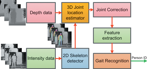
Figure 4. Pipeline for outlier removal. Inputs to “3D Joint location estimator” remain the same as in .Figure 3

Body-tracking Using Intensity and Depth Data

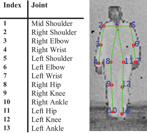
Figure 3 describes the workflow of the gait recognition methodology for the flash lidar data. We start with the 2D skeleton detection and 3D joint location estimation steps. For a lidar sequence $V$ with $f$ frames, there exists intensity $I=[I_1,I_2,\dots ,I_f]$, and depth $R=[R_1,R_2,\dots ,R_f]$, where $I_i$ and $R_i$ represent intensity and depth data at frame $i$. Intensity data are fed into a 2D skeleton detector. We leverage OpenPose, a state-of-the-art real-time pose detector, to fit a skeleton model and extract the location of body joints. In Figure 5, the top row shows examples of correctly detected skeleton joints. As we can see in this figure, OpenPose provides a skeleton model of 18 joints, where 5 of the joints represent the nose, eyes, and ears. It is important to note that some of the points in a skeleton model might not represent an actual joint. In general, these points are a set of anatomical landmarks. However, for convenience and consistency with literature, we call all of these points joints. The skeleton model that we adopt in this paper includes 13 joints. The reason for such choice is the fact that face joints are missing from a large majority of our samples. Figure 6 illustrates the skeleton model that we use in this work. Given $I_i$ as the input to the skeleton detector, the output is the joint location coordinates that can be represented with the following vectorized form

(1) $J_i=[x_k,y_k{]}_{k=1}^M\in {\mathrm{\Re }}^{2N}$(1)

Figure 5. Top row: sample frames with correctly detected skeletons, bottom row: frames with faulty skeletons.

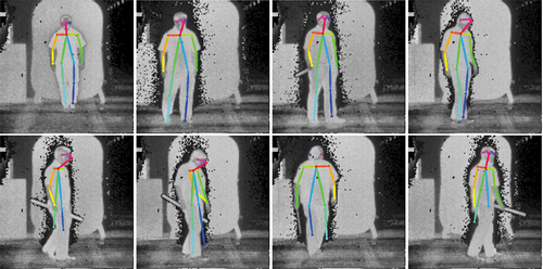
Figure 6. The skeleton model that we use in this work. Left: index of each joint in the skeleton model. Right: skeleton model in a sample frame.

where $(x_k,y_k)$ are the coordinates of the $kth$ joint in the image frame of reference, and $M$ represents the number of joints. Considering the structural analogy between the 2D digital camera and 3D flash lidar, the pinhole camera model can be applied to the flash lidar camera as well (Jang et al. 2017). Therefore, the relation between a point in the real-world 3-dimensional coordinate system and its 2-dimensional location in the image reference frame can be described by the following equation

(2) $L_j^i=\frac{L{p}_j^i}{f}\times D_{camera}^i$(2)

where $f$ is the focal length of the camera and $D_{camera}^i$ is the depth value of joint $i$. $L{p}_j^i$ represents the location of joint $i$ in direction $j$ in the image coordinate system. Here $j$ is in the $x$ or $y$ direction, and $L^i$ in the $z$ direction equals the depth value at the location of joint $i$. Furthermore, the viewpoint angle can be described by

(3) ${\theta }_{aov}=2arctan(\frac{N_{pixels}}{2f})$(3)

where $N_{pixels}$ is the number of pixels in the $j$ direction and ${\theta }_{aov}$ represents the angle of view. By combining (2) and (3), we can project the 2-dimensional coordinates of joints into the real-world coordinates (McCollough 1893). $L_j^i$, the real-world location of joint $i$ in direction $j$, can be calculated according to the following equation

(4) $L_j^i=\frac{2}{N_{pixels}}\times tan(\frac{{\theta }_{aov}}{2})\times L{p}_j^i\times D_{camera}^i$(4)

As we discussed earlier, the quality of the resulting skeleton and the joint localization are negatively affected by several factors. The features that are computed using the acquired skeletons are plagued with erroneous measurements. Therefore, gait recognition based on the computed defective skeletons results in a high rate of false positives. To resolve this problem, we present a filtering mechanism that employs polynomial interpolation and robust statistics to correct for noisy and missing measurements in time sequences of joint coordinate values. We will describe the filtering mechanism in Correction of anatomical landmarks.

Feature Extraction

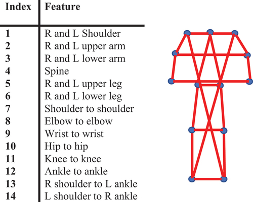
To evaluate the performance of the proposed method, we use two different sets of feature vectors: length-based feature vectors and vector-based feature vectors. The length-based feature vector consists of a set of limb lengths and distance between selected joints in the skeleton that are not directly connected. Figure 7 describes the components of the length-based feature vector. This set includes static limb length features and some other distance attributes that change during motion, and encodes information about postures.

Figure 7. Illustration of length-based feature vectors. Left: description of each feature (L and R refer to the left and right joints, respectively). Right: illustration of the features.

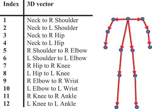
The second set of feature vectors is vector-based. Each feature is a 3-dimensional vector, with origin and termination at two skeleton joints. Compared to distance-based features (Yang et al. 2016), or the angle-based attributes (Ball et al. 2012), vector-based features encode the angle and distance between selected joints of the skeleton. Figure 8 lists the joints that form each of the three-dimensional vectors in the vector-based feature vector. Unlike features in Kumar and Venkatesh Babu (2012) that are computed with respect to a reference joint, the vectors in the vector-based feature here are formulated between different joints, mimicking the limb vectors in the skeleton model.

Figure 8. Illustration of vector-based feature vectors. Left: description of each feature (L and R refer to the left and right joints, respectively). Right: illustration of the features.

Correction of Anatomical Landmarks

Let $L$ be a matrix of the size of $39\times F_n$, where each row represents the time sequence of one joint in one of the directions $x,y,$, and $z$, extended over $F_n$ frames. Since each skeleton consists of $13$ joints, there are in total $39$ joint coordinate time sequences. To correct for missing joint location values and noisy outliers in a given video, we perform filtering of joint location on each row of the corresponding $L$ matrix. Let $L_m$ represent the $m$ th row of $L$

(5) $L_m=[L_m(t){]}_{t=1}^{F_n}{L}_m(t)\in \mathrm{\Re }$(5)

Given the joint location sequence $L_m$, we find the sorted location of all the nonzero elements. We define $n_{L_m}$ as the sorted set of all the indices in $L_m$ with a non-zero value (each index corresponds with one time instant $t$) such that

(6) $\begin{array}{c}{n}_{L_m}=[n_1,n_2,\dots ,n_R]\\ n_1<n_2<\dots <n_R\\ n_i\in [1,2,\dots ,F_n];i\in [1,2,\dots ,R]\end{array}$(6)

where $R$ is the number of non-zero elements in $L_m$. Next, between any two nonzero values with nonconsecutive indices along time, we fit a first-order polynomial through the least squares criterion

(7) $\left(\begin{array}{cc}{n}_r& 1\\ n_s& 1\end{array}\right)\left(\begin{array}{c}{p}_1\\ p_2\end{array}\right)=\left(\begin{array}{c}{L}_m(n_r)\\ L_m(n_s)\end{array}\right)$(7)

where $n_r,n_s\in n_{L_m}$ and $n_s-n_r>1$. $L_m(n_r)$ and $L_m(n_s)$ are the values of $L_m$ at $n_r$ and $n_s$, respectively. $p_1$ and $p_2$ can be obtained by finding the least squares solution to the system of equations in (7). The polynomial fitting is performed over any two nonconsecutive time indices in the sorted time indices array of non-zero elements of $L_m$. Finally, we employ RLowess (locally weighted scattered plot smoothing) filter (Cleveland 1979) to smooth the resulting joint location sequence and alleviate the effect of remaining lower-amplitude spikes in $L_m$. RLowess assigns a value to each point by locally fitting a first-order polynomial, utilizing weighted least squares. Weights are computed using the median absolute deviation (MAD), which is a robust measure of variability in the data in the presence of outliers. The robustness of weights is critical due to the existence of smaller-amplitude spikes that act as outliers.

The described filtering procedure will effectively correct measurements in joint location time sequences. Furthermore, when pose-detector fails to detect a skeleton model, the joint location filtering can interpolate the missing skeleton joint locations. Figure 9 illustrates the result of filtering on samples of joint location coordinate time sequences.¹ As we can see in this figure, the original joint location sequences are noisy, containing many missing values and outliers. In the third row of Figure 9, we can also see the sample frames with missing skeleton joints in the image reference frame. As we observe in the last row, the missing joints are interpolated successfully through the filtering mechanism. We can also see two samples where a whole skeleton is recovered through the joint location correction. The joint location correction can be easily applied in the cases of occlusion for the one-subject and multi-subjects scenarios. While in this study the missing joint locations are the result of erroneous joint localization, it can be the result of occlusion. For most of the cases, the interpolation of missing or noisy joints follows the correct joint locations. However, there exist cases where the obtained localization results are not accurate. Figure 10 shows some failure examples in joint localization correction. The majority of such failure cases are the result of the existence of a considerable number of successive frames with missing or noisy joints that make the joint correction prone to defective measurements. However, even for failure cases, at least half of the joints are predicted correctly. This can enhance the likelihood of correct identification compared to the original localization of the joints.

Figure 9. Effect of joint location sequence filtering. From top: sample joint location sequences before (first row) and after (second row) joint location sequence filtering (each joint location sequence corresponds with one coordinate ($x,y,z$) of the location of one joint through time). Notice the abundance of missing values in the first row, which are shown as missing sections of the plotted signal, that have been recovered through the joint correction (figures in the second row). The last two rows show samples of faulty and missing skeleton joints before (third row) and after (bottom row) joint location sequence filtering.

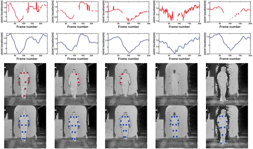
Figure 10. Failure examples of the joint location correction filtering. Sample frames of skeleton joints, before (top) and after (bottom) the joint location correction.

Computational Complexity of Joint Correction

The main computational bottleneck is in the last step of joint correction filtering, where we use Rlowess for smoothing the curve of joint location time sequences, and alleviate the effect of outliers with $O(Nlog(N)+3N(d+1)k)$ computational complexity. Here, $N$ is the number of points in a joint location time sequence, $d$ is the degree of the polynomial used in the regression (here $d=1$), and $k$ is the number of k-nearest point or length of each span in the local regression smoothing ($k$ is constant and the same for all the points) (Smolik, Skala, and Nedved 2016).

Incorporating the Dynamics in Gait Recognition for the Corrected Skeletons

As humans, we recognize a familiar person not just by looking at their body measurements like height; we also incorporate the way that people move their bodies during activities, such as walking. In the gait recognition language, the first set of features that are computed from body measurements like limb lengths or height are called static features. Attributes like step length or speed that comprise the motion of gait from one posture to another posture, are dynamic features. When individuals with approximately the same body measurements are considered, dynamic features are critical for successful gait recognition. Speed, step length, and stride length are among the widely used features to incorporate the dynamic of the motion (Koide and Miura 2016; Preis et al. 2012). Computing moments like mean, maximum, and variance of selected features over each gait cycle (Chi, Wang, and Q-H Meng 2018; Sinha, Chakravarty, and Bhowmick 2013; Yang et al. 2016) is another common practice in the majority of model-based methods. The time sequence of the distance between the two ankle joints is a commonly employed attribute to compute the gait cycle. This practice has repeatedly proven to be successful in encoding the dynamic of motion, achieving high accuracy in gait recognition. However, this analysis is commonly performed on a clean dataset with a low level of noise and a few to none outliers. Such datasets are commonly recorded under controlled conditions, like limited directions of motion in front of a camera.

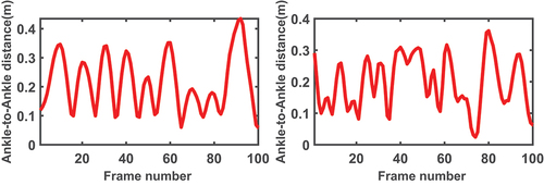
Figure 11 shows examples of the time sequence of the ankle to ankle distance for lidar data after joint location correction. The sequence on the left shows a periodic pattern. However, like the sequence on the right side of Figure 11, some examples lack a clear cyclic pattern. As Chi et al. (Chi, Wang, and Q-H Meng 2018) discussed, variations in different walking factors such as walking direction, walking speed, and step length can cause aperiodicities in the walking patterns. This can cause complexities in the interpretation of the motion, such as in gait cycle computation. In addition to such intra-personal variations in the gait, with the flash lidar data, there is a considerable amount of consecutive frames with a missing skeleton in each sequence. This will cause the result of joint sequence correction prone to noisy measurements, and therefore, it will exacerbate the problem of the observed acyclic patterns. Considering the sequences in Figure 11, irrespective of a sequence being periodic or aperiodic, we consider a gait cycle as a local time sequence with three consecutive local maxima. To compensate for large variations in the gait cycle throughout one sequence of walking, we incorporate statistics that are robust to noisy data. In addition to the commonly employed statistics of mean, standard deviation, and maximum, we also include median, upper, and lower quartiles that are robust to noisy data. We build feature vectors that comprise mean, standard deviation, maximum, median, lower quartile, and upper quartile of each feature over every gait cycle. Later, we will show that the resulting feature vectors can improve the classification scores over the feature vectors with only non-robust moments.

Figure 11. Two examples of the ankle to ankle distance sequence of flash lidar data after joint correction. While the graph on the left presents a clear periodic pattern, the sequence on the right lacks such a pattern.

Outlier Detection and Exclusion

Outliers are a set of observations that cannot be described by the underlying model of a process. While in some applications, i.e. surveillance and abnormal behavior detection, outlier observations can be of interest and are kept for further investigation, there are situations that outliers are the result of faulty measurements or caused by noise. The latter type of outliers has to be detected and removed before model estimation because the models that are estimated utilizing the data which is contaminated by such outliers are not accurate and generate many false predictions. For gait recognition, one common approach is to remove outlier measurements from the collected data by setting some measurement thresholds (Chi, Wang, and Q-H Meng 2018; Semwal et al. 2017; Yang et al. 2016). The second row in Figure 5 presents some of the examples of faulty skeletons that are the result of erroneous joint localization. Furthermore, there are frames with missing skeletons.

For comparison, and as an alternative approach to deal with noisy and missing joint location measurements in our dataset, we employ the Tukey method along with some pre-filtering to detect outliers in the feature vectors. We choose Tukey’s test, in particular, to avoid making any assumption about the underlying distribution of the features. Based on Tukey’s test, an outlier is any value that is below $Q{u}_{low}-1.5\times IQR$ or above $Q{u}_{up}+1.5\times IQR$, where $IQR=Q{u}_{up}-Q{u}_{low}$ stands for the interquartile range. $Q{u}_{low}=\frac{1}{4}(n+1{)}^{th}$ term or lower quartile, and $Q{u}_{up}=\frac{3}{4}(n+1{)}^{th}$ term or upper quartile are defined on an ordered set of $n$ terms.

Outlier Removal for Length-based Features

We define $Jd=[J{d}_1,J{d}_2,\dots ,J{d}_P]$ as a feature vector, where $P$ is the number of features in $Jd$, and $J{d}_i$ is the Euclidean distance between two skeleton joints. Before applying Tukey’s test, we first remove all the frames with missing skeletons. Next, Tukey’s test is employed on each feature. $Jd$ is not an outlier if

(8) $Tukey(\{J{d}_i{\}}_{i=1}^P)={\mathbf{0}}_{P}whereJ{d}_i\in {\mathrm{\Re }}^{+}$(8)

where ${\mathbf{0}}_P$ is a zero vector of length $P$. $Tukey(J{d}_i)=0$ means that feature $J{d}_i$ passed the Tukey’s test, or $J{d}_i$ is not an outlier. Based on Equation (8)(8) $Tukey(\{J{d}_i{\}}_{i=1}^P)={\mathbf{0}}_{P}whereJ{d}_i\in {\mathrm{\Re }}^{+}$(8) , feature vector $Jd$ is a non-outlier, if all of its feature components are non-outliers. In other words, $Jd$ is an outlier if there exists a $J{d}_i$, such that $Tukey(J{d}_i)=1$. As we will show later, while outlier removal will improve gait recognition scores, it comes at the cost of eliminating a considerable portion of the data.

Outlier Removal for Vector-based Features

There are cases where the components of a feature vector are vectors. This happens if we compute the 3-dimensional vectors between skeleton joints. In other words, we have a $3\times Q$ vectorized matrix $J{v}^{3D}=[J{v}_1^{3D},J{v}_2^{3D},\dots ,J{v}_Q^{3D}]$ of the joint coordinates. $Q$ is the number of 3-dimensional vectors in $J{v}^{3D}$, and $J{v}_i^{3D}$ represents the $ith$ column, which is the 3-dimensional vector between two skeleton joints

(9) $J{v}_i^{3D}=[x_i,y_i,z_i]\in {\mathrm{\Re }}^{3N}$(9)

We need to treat each of the 3-dimensional vectors as one entity, rather than treating each dimension separately.

To detect outliers for this set of features, we use the concept of marginal median. The marginal median of a set of vectors is a vector where each of its components is the median of all the vector components in that direction. We then use cosine distance to calculate vector similarity between each set of 3-dimensional vectors and their corresponding median vector. We define $J{v}^{median}$ as the marginal median over all the given $J{v}^{3D}$ feature vectors

(10) $S^{3D}=cos(J{v}_i^{median},J{v}_i^{3D}){|}_{i=1}^Q$(10)

where $S_i^{3D}=cos(J{v}_i^{median},J{v}_i^{3D})$ is the cosine similarity between i element of feature vector $J{v}^{3D}$ and $J{v}^{median}$. Then, Tukey’s test is employed on the cosine similarity measures, and a feature vector is labeled as an outlier if at least one of its features is an outlier. The algorithm below describes outlier detection on the feature vectors built from 3-dimensional vectors.

Outlier Detection for Vector-based Features

1. Over all the given feature vectors, calculate the marginal

median vector. Call this vector $J{v}^{median}$

2. For each 3D vector $J{v}_i^{3D}$ in each feature vector $J{v}^{3D}$,

calculate $cos(J{v}_i^{median},J{v}_i^{3D})$; save the results in one

row of $S$.

3. Employ Tukey’s test on each row of $S$.

4. A given feature vector $J{v}^{3D}$ will pass Tukey’s test if

its corresponding row in $S$ passes Tukey’s test.

Results and Discussion

The proposed joint correction is evaluated on two datasets: our flash lidar dataset (Evaluation on flash lidar data), and IAS-Lab (Evaluation on IAS-Lab) collected by a Kinect camera (Munaro et al. 2014a). While our focus is not on Kinect modality, due to the lack of publicly available flash lidar data for gait recognition, we evaluate the performance of the joint correction methodology on IAS-Lab RGB-ID. To evaluate the performance of the joint correction filtering on IAS-Lab, we remove the whole skeletons in consecutive frames and manually add noise to skeleton joints.

Evaluation on Flash Lidar Data

In this subsection, we first expalin about TigerCub 3D flash lidar as a modality that can collect intensity and depth data, simultaneously. Next, we describe the test setup and collected flash lidar dataset in Test setup and dataset and study the effect of joint correction by looking at the gait identification results before and after applying GlidarPoly and also present the results with outlier removal (Effect of joint correction on gait recognition). We then look at the effect of integrating robust statistics to capture motion dynamics in Effect of the robust statistics integration. Finally, in Effect of the number of training samples, we investigate the effect of the number of training samples on the performance of the proposed method for gait recognition.

TigerCub 3D Flash Lidar

As a depth-based modality, Kinect removes the hurdle of model fitting due to the direct estimation of joints coordinates. However, the working range of Kinect is limited. Furthermore, the depth data of Kinect is not reliable in outdoor environments, because the system is unable to distinguish the infrared light of the sensor from infrared radiation present in the outdoor environment (Fankhauser et al. 2015). In other studies, high-quality real-time skeleton joint positions are acquired by motion capture (mocap) (Balazia and Plataniotis 2017; Krzeszowski et al. 2014). In terms of applicability, mocap is limited to a laboratory environment. Unlike mocap, flash lidar has been extensively used for outdoor applications. Compared with Kinect, a flash lidar camera has a significantly extended range ($>1000$ meters) and its performance is not degraded in outdoor environments due to the irradiance of the background (Horaud et al. 2016).

The TigerCub is a light-weight 3D flash lidar camera that provides real-time depth and intensity data, using eye-safe Zephyr laser (Horaud et al. 2016). The performance of the camera is not affected by the lack of light at night, or in the fog or dust. This sensor has a focal plane of $128\times 128$ and can acquire up to 20 frames per second.

Test Setup and Dataset

The dataset in this work has been recorded using a single TigerCub 3D flash lidar camera. The camera is in a fixed location during all the actions. There are in total $34$ sequences of walking actions performed by $10$ subjects, captured at the rate of $15$ fps. The recording includes walking action of three main categories: walking toward and away from the camera, walking on a diamond shape, and walking on a diamond shape while holding a yardstick with one hand. Figure 12 illustrates the paths of walking for the two cases of walking forward and backward (walking toward and away from the camera) and the diamond walking. For those frames in which subjects walk toward and away from the camera, most of the views are from the front and back of the person, with some frames of side views when the subjects turn away. The sequences with walking on a diamond shape include frames with a wider range of views. This will offer a wider range of poses as is shown in Figure 13. The number of frames per video is different, ranging from $130$ to $498$ frames. Each frame has two sets of data, intensity, and depth, both with the same number of pixels. The intensity data are presented in gray-scale, and the depth data show the distance of each point in the field of view from the camera sensor.

Figure 12. Illustration of two types of waIking paths: walking forward and backward (dashed line) and diamond walking (solid line).

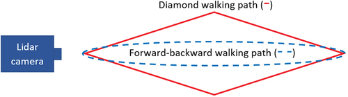
Figure 13. Sample frames of diamond walking that captures a range of different poses.

Effect of Joint Correction on Gait Recognition

To evaluate the performance of the proposed joint correction, we carry out a comparison with four state-of-the-art relevant gait recognition methods before and after employing skeleton joint correction. These methods are as follows: Preis (Preis et al. 2012), Ball (Ball et al. 2012), Sinha (Sinha, Chakravarty, and Bhowmick 2013), and Yang (Yang et al. 2016). Preis et al. use a set of static features, plus step length and speed as dynamic features. Ball et al. use the moments of six lower body angles. Sinha combines the features in Preis et al. (2012) and Ball et al. (2012) with their area-based and distance between body segments features. Yang et al. utilize selected relative distance on different motion directions. To compare the performance of different methods, we consider the average accuracy and F-score. We also evaluate the performance of the proposed outlier removal method. We use $75\mathrm{\%}$ of the sequences for training and the rest for testing, and hire 10-fold cross-validation for training. To ensure the generalization of the proposed method, the classifier is tested on a type of walking that it was not trained on. Support vector machine (SVM) with the radial basis function (RBF) kernel is adopted as our classifier. We also employed a linear kernel and, in most of the cases, we acquired either the same or lower accuracy with the linear kernel. In the first experiment, we consider the per-frame (one-shot) scenario for both length-based and vector-based features and do not incorporate motion dynamics in our features.

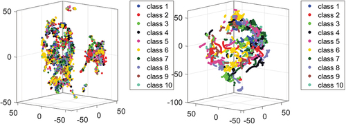
Figure 14 and 15 show t-SNE visualization of length-based and vector-based features for the training data before and after joint location correction. Some of the interesting observations from these visualizations are as follows:

• There is a high level of the inter-class intersection before joint correction, which is transformed into a wider separation among classes after the joint location correction.

• In the right graph of Figure 15, we see class 9 that is non-homogeneously scattered, which makes it more difficult to find the decision boundary. This is one of the reasons that we get a lower accuracy for this class (the per-class accuracy is presented in Table 3) and overall lower accuracy for the whole dataset.

• In Figure 15, we observe two separate clusters that are transformed into a single one after joint correction.

• The transformed features are well separated, which shows we do not necessarily need a more sophisticated classifier.

Table 1. Correct identification scores for the proposed features (**) and the other methods. LB and VB stand for the length-based and vector-based feature vectors, respectively. Results are shown for the original (without joint correction) and after applying GlidarPoly. We also included the results with the proposed features after outlier removal.

Method	Average Accuracy (%)	Average F-score(%)
Original
Preis et al. 2012	30.26	23.67
Ball et al. 2012	27.30	23.21
Sinha, Chakravarty, and Bhowmick 2013	62.02	55.44
Yang et al. 2016	62.10	57.37
**LB	55.20	52.20
**VB	65.93	63.72
After outlier removal
**LB	66.63	61.21
**VB	80.70	75.22
After GlidarPoly correction
Preis et al. 2012	40.77	36.21
Ball et al. 2012	32.55	32.49
Sinha, Chakravarty, and Bhowmick 2013	80.11	80.40
Yang et al. 2016	75.79	72.75
**LB	73.84	70.66
**VB	84.07	80.49

Table 2. Correct identification scores with statistics of features computed over gait cycle. LB and VB stand for the length-based and vector-based feature vectors, respectively. The 3-statistic case refers to computing only mean, maximum, and standard deviation of each feature over every gait cycle. The 6-statistic scenario adds median, lower and upper quartile to the initial three statistics.

Method	Average Accuracy (%)	Average F-score (%)
LB (3 statistics)	75.27	73.20
LB (6 statistics)	76.03	74.88
VB (3 statistics)	83.32	80.91
VB (6 statistics)	89.12	87.06

Table 3. Correct identification scores for each class of subject for the single-shot scenario of vector-based features. The minimum and the next-to-lowest accuracy and F-score are underlined.

Subject #	Average Accuracy (%)	Average F-score (%)
Subject 1	93.85	96.83
Subject 2	80	79.69
Subject 3	79.23	69.36
Subject 4	74.62	64.03
Subject 5	93.08	82.88
Subject 6	76.92	64.52
Subject 7	100	84.69
Subject 8	76.92	85.29
Subject 9	66.92	78.61
Subject 10	82.31	88.25

Figure 14. T-SNE visualization of the length-based feature before (left) and after (right) applying joint correction. There is a high level of inter-class intersection before joint correction (left) that is mostly resolved after correcting joint location, creating clusters that are more distinctive (right).

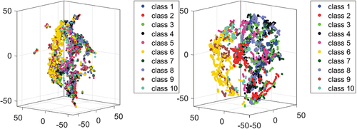
Figure 15. T-SNE visualization of the vector-based feature before (left) and after (right) applying the joint correction. Before joint correction, high inter-class intersection and intra-class separation is observed (left). Joint correction transforms features into well-separated clusters (right).

Table 1 shows the correct identification scores for the original (without the joint correction), with outlier removal, and after applying GlidarPoly. As we can see, the identification scores are generally low when features are computed from the skeleton data without skeleton joint correction. This is due to the existence of a considerable number of noisy and missing skeletons. We also observe that while outlier removal can improve the identification scores, it is not as effective as the joint correction. This might be caused by noisy features that still exist after outlier removal. Furthermore, outlier removal eliminates more than $40\mathrm{\%}$ of the data, which can be problematic when data are limited.

The results in Table 1 demonstrate the effectiveness of joint correction, where the correction process improves the gait identification scores in all of the cases. Among the evaluated methods, the performance of Ball et al. (2012) does not improve as much as the other approaches. In Ball et al. (2012), the authors use six angles between lower body joints as features and compute three moments of each angle over every gait cycle. We see in Figure 6 that the adopted skeleton model in our work lacks foot joints that are essential to estimate two of the angles in Ball et al. (2012). To calculate these angles, we estimate the floor plane and use the normal vector to the plane. We speculate that the error in this estimation might also result in lower performance of this method compared to the others. Furthermore, it was reported before that distance-based features might work better than angle-based features, in particular, when the number of subjects is relatively low (Dikovski, Madjarov, and Gjorgjevikj 2014). Joint angles are also prone to changes in the walking speed (Han 2015; Kovač and Peer 2014). Results also show that vector-based features outperform length-based features. Furthermore, while our feature vectors do not contain the dynamics of the motion, vector-based features still outperform methods that incorporate temporal information by computing moments of features over the gait cycle.

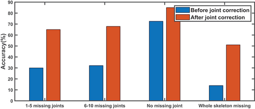
Figure 16 compares the classification accuracy based on the number of missing joints in the original detected skeletons before and after applying GlidarPoly for the joint location correction. This graph shows that the accuracy improves in all of the groups after the joint location correction. This confirms the effectiveness of GlidarPoly in improving skeleton joint localization. It should be noted that samples with no missing joints also include noisy joint data. The sudden jumps in the joint time sequence samples in the top row of Figure 9 present examples of such noisy behavior in the original joint localization.

Figure 16. Comparison of classification accuracy for vector-based features based on the number of missing joints in the original skeletons, before and after applying GlidarPoly for joint correction. The samples with no missing joints also include noisy samples. All cases show improvement after applying the joint location correction.

Effect of the Robust Statistics Integration

As we discussed earlier, to integrate the motion dynamics after applying the joint correction, we compute six statistics of our features over each gait cycle. Table 2 presents the identification scores when the statistics of length-based and vector-based features are computed over each gait cycle. By comparing the classification scores, we realize that adding the median, upper, and lower quartile to commonly employed statistics of mean, maximum, and standard deviation can improve the identification results after skeleton correction. The average per-class accuracy and F-score for the single-shot (per-frame) case are summarized in Table 3. We also present the per-class accuracy and F-score for the gait cycle statistics in Table 4. By comparing the per-class classification scores for the single-shot and statistics over the gait cycle, we also see that the minimum per-class accuracy and F-score are improved by $4.5\mathrm{\%}$ and $10.97\mathrm{\%}$ as a result of employing gait cycle statistics. This indicates that by employing features that encode motion dynamics, we can build a more reliable model compared to the case that only considers static features.

Table 4. Correct identification scores for each class of subject for the statistics of vector-based features over the gait cycle. The minimum and the next-to-lowest accuracy and F-score are underlined.

Subject #	Average Accuracy (%)	Average F-score (%)
Subject 1	71.42	83.33
Subject 2	85.71	80
Subject 3	85.71	92.31
Subject 4	85.71	75
Subject 5	100	93.33
Subject 6	100	82.35
Subject 7	100	77.78
Subject 8	85.71	92.31
Subject 9	85.71	92.31
Subject 10	78.57	88

Effect of the Number of Training Samples

It is essential to investigate how the designed model or the selected features perform under limited data availability. To address this concern, we examine the effect of the number of training samples on the performance of the vector-based features, both for the single-shot approach as well as the statistics over a gait cycle.

In Figure 17, the left graph presents the single-shot identification accuracy as a function of the number of training examples, for several number of test samples in $[100,1000]$ range. For a given number of test samples, the accuracy of identification improves as we increase the number of training data. A test sample size equal to or larger than 200 frames appears to be a proper choice empirically, as the accuracy trend is shown to be more stable. We also observe that the best performance is obtained with a training set of 1000 samples, irrespective of the number of test data.

Figure 17. Average classification accuracy for different sizes of training sample sets given multiple numbers of test examples for the single-shot (left), and statistics over the gait cycle (right) scenarios. Both plots are acquired for vector-based features.

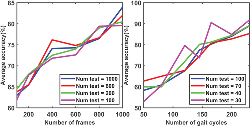
In Figure 17, the right graph illustrates the same experiment with a various number of gait cycles. This graph shows classification accuracy when the statistics of features over a gait cycle are considered as the feature vectors. The number of training cycles changes over the range of $[50,230]$. We observe that regardless of the number of test samples, with a training sample of at least $200$ gait cycles, we can acquire the highest accuracy with this feature. This limitation can be problematic when the available number of gait cycles per subject is severely limited.

Evaluation on IAS-Lab

IAS-Lab RGB-ID dataset includes three sets, “Training,” “TestingA,” and “TestingB” of 11 different subjects. Subjects perform walking action and rotate on themselves during walking. The outfits of the subjects in “TestingA” are different from their outfits in “Training” set. “TestingB” sequences are captured in a different room, with subjects wearing the same outfits as in the “Training” sequences. Furthermore, some sequences in “TestingB” are recorded in a dark environment. First, we compute the single-shot rank-1 identification accuracy for our vector-based and length-based features and compare it with several state-of-the-art methods with the original data in Single-shot identification with IAS-Lab. Next, we manually add noise to some of the skeleton joint locations and randomly remove some of the other joint location information. Then, we apply GlidarPoly, and compare the results of gait recognition with the corrupted joints and after employing GlidarPoly in Effect of joint correction on gait recognition. Finally, we look at the effect of integrating robust statistics to capture motion dynamics after applying GlidarPoly for skeleton correction in Effect of the robust statistics integration.

Single-shot Identification with IAS-Lab

Table 5 shows the single-shot rank-1 identification accuracy for our length-based and vector-based features (the last two rows), and several other RGB and depth-based methods on the IAS-Lab dataset. All the results with the RGB-based features (features that are extracted from RGB images) are reported based on Ancong, Zheng, and Lai (2017). As we can see, 2D RGB-based features achieve better results on “TestingB” compared with “TestingA” where subjects are wearing different outfits. This is because changes in the outfit can affect the consistency of these types of features. $D^{13}$ skeleton feature (Munaro et al. 2014b) consists of 11 length-based features and 2 ratios of length-based features. PCM $+$ Skeleton (Munaro et al. 2014a) adds the point cloud matching to these skeleton-based features of Munaro et al. (2014b). In Pala et al. (2019), the authors use a weighted combination of 3D skeletal and 3D face features to improve person re-identification. The 3D CNN (Haque, Alahi, and Fei-Fei 2016) is trained on the 3D point cloud, while 3D RAM (Haque, Alahi, and Fei-Fei 2016) is a recurrent attention model trained on 4D tensors of 3D point cloud over time. ED $+$ SKL (Ancong, Zheng, and Lai 2017) is another depth-based feature, computed from eigen-depth and skeleton-based attributes. In Zheng et al. (2019), an attentional Recurrent Relational Network-LSTM is designed that can model the spatial information and temporal dynamics in skeletons, simultaneously. 3D pose data concatenated with several other spatio-temporal features are fed as the input to a CNN for gait recognition in PoseGait (R. Liao et al. 2020).Rao et al. (2021) present a self-supervised method with locality-awareness to learn gait representations. In the last two rows, we present the results with our length-based and vector-based features using NN (nearest neighbor) and SVM classifiers. For the NN classifier, we use the Manhattan distance with five nearest neighbors, similar to our previous study (Nasrin et al. 2019). The results show that Reverse Reconstruction (Rao et al. 2021) outperforms other methods on “TestingA” where subjects are wearing outfits different from the training set. Our vector-based feature comes second in terms of performance for “TestingA,” with $6.46\mathrm{\%}$ higher accuracy compared with the next best performing method (ED+SKL). On “TestingB” (where there are changes in the illumination), our length-based and vector-based features acquire the first and second highest accuracies compared with the other methods.

Table 5. Single-shot identification: Rank-1 identification accuracy for the proposed features, several RGB-based (features that are extracted from RGB images), and depth-based (features that are extracted using depth data, e.g. skeleton-based features) features for IAS-Lab RGBD-ID “TestingA” (different outfits) and “TestingB” (different rooms, various illuminations) sets. With (Rao et al. 2021), we only report the best results that was achieved by Reverse Reconstruction method. With our features, we only show the best results that was achieved by NN (Nearest Neighbors) and SVM (Support Vector Machine) for the Length-based and Vector-based features, respectively.

Method	TestingA	TestingB
RGB-based features
HOG (Oreifej, Mehran, and Shah 2010; Ancong, Zheng, and Lai 2017)	31	47.21
Gabor-LBP (Zhang and Shutao 2011; Ancong, Zheng, and Lai 2017)	28.71	51.38
LOMO (S. Liao et al. 2015; Ancong, Zheng, and Lai 2017)	26.37	30.97
Depth-based features
$D^{13}$ Skeleton (NN) (Munaro et al. 2014b)	22.5	55.5
$D^{16}$ Skeleton+Adaboost (Pala et al. 2019)	27.4	39.2
PCM+Skeleton (Munaro et al. 2014a)	25.6	63.3
$3D$ CNN (Haque, Alahi, and Fei-Fei 2016)	44.2	56.2
$3D$ RAM (Haque, Alahi, and Fei-Fei 2016)	48.3	63.7
ED+SKL (Ancong, Zheng, and Lai 2017)	48.75	58.65
Multi-layer LSTM (Zheng et al. 2019)	34.4	30.9
PoseGait (R. Liao et al. 2020)	41.4	37.1
Reverse Reconstruction (Rao et al. 2021)	60.1	62.5
Length-based (NN)	46.61	70.64
Vector-based (SVM)	55.21	67.71

Effect of Joint Correction on Gait Recognition

To evaluate the performance of the joint correction filtering on IAS-Lab, we added some errors using Gaussian distribution, to randomly selected joints. Furthermore, we randomly removed the joint location information of some other joints. Table 6 presents the single-shot rank-1 identification accuracy on the IAS-Lab with the added noise and after applying GlidarPoly for joint location correction. As the results show, the identification scores improve considerably after applying GlidarPoly. We see the identification accuracy after applying GlidarPoly is close to the results with the original data (the last two rows of Table 5), which again proves the effectiveness of the proposed joint correction filtering mechanism. For the length-based features in “TestingA” set, we see that the results with GlidarPoly are even better than the results with the original uncorrupted data in Table 5. This might indicate the removal of some of the noise that exists in the original data. The results in these tables show that improvement is more pronounced with “TestingB” in IAS-Lab. Furthermore, length-based features in general see a higher percentage of improvement compared with the vector-based features. Table 6 shows that identification accuracy improves in the range of $[15\mathrm{\%},33\mathrm{\%}]$ after applying GlidarPoly to correct the faulty joint locations in IAS-Lab.

Table 6. Single-shot identification: Rank-1 identification accuracy for the proposed features on IAS-Lab RGBD-ID “TestingA” (different outfits) and “TestingB” (different rooms, various illuminations) before (with added noise and removed joints) and after applying GlidarPoly for correction. We only show the best results that was achieved by NN (Nearest Neighbors) and SVM (Support Vector Machine) for the Length-based and Vector-based features, respectively.

Method	TestingA	TestingB
With added noise
Length-based (NN)	23.86	30.18
Vector-based (SVM)	39.19	46.35
After applying GlidarPoly
Length-based (NN)	48.24	63.93
Vector-based (SVM)	52.58	62.34

Effect of the Robust Statistics Integration

Table 7 shows the rank-1 identification scores after computing the 6 statistics of length-based and vector-based features of corrected skeletons over the gait cycle for “TestingA” and “TestingB” sets. By comparing the results with the single-shot identification accuracy after joint correction in Table 6, we only observe improvements in two cases (cases with improvements are shown in boldface.) As we discussed earlier in Effect of the number of training samples and illustrated in Figure 17, our evaluation shows that we need an order of $10$ gait cycles for training to acquire improvement over the single-shot scenario. To achieve this improvement on the lidar dataset, we need on average at least $20$ gait cycles per subject. While in our lidar dataset there is only one subject with less than $20$ gait cycles for training, in IAS-Lab dataset there are 3 subjects with such a condition. Therefore, we observe fewer cases of improvement in IAS-Lab dataset compared with our flash lidar data.

Table 7. Rank-1 identification accuracy using the $6$ statistics of the proposed features on IAS-Lab “TestingA” (different outfits) and “TestingB” (different rooms, various illuminations) after joint location correction. We only show the best results on average that was achieved by NN (Nearest Neighbors) and SVM (Support Vector Machine) for the Length-based and Vector-based features, respectively.

Method	TestingA	TestingB
Length-based (NN)	53.88	66.88
Vector-based (SVM)	46.89	61.29

Discussion

Our experiments show that GlidarPoly, the proposed filtering method for skeleton correction, is effective in improving the quality of noisy skeleton joints and recovering missing joints and therefore enhancing gait recognition results. We also observed that while outlier removal improves gait recognition scores, it is still inferior to skeleton correction with GlidarPoly. Outlier removal can be a practical solution when outlier and noisy frames are a small portion of the collected data. However, data elimination can raise serious issues when a considerable portion of the data are outliers (as with our dataset). In particular, when outliers exist in consecutive frames, which is common in the flash lidar dataset, outlier removal results in the elimination of temporal information that is critical for applications such as gait recognition. As we saw in Table 2 , once we employ temporal information after joint correction, outlier removal results in even lower recognition accuracy as compared with the joint location correction.

We also observed that incorporating robust statistics such as median and upper and lower quartiles to the more common feature moments can provide a richer representation of temporal information after skeleton correction. In Figure 18, we show the performance of three sets of feature statistics over every gait cycle after applying GlidarPoly on the lidar data, and “TestingA” (different outfits) and “TestingB” (different rooms, various illuminations) in IAS-Lab. We use NN and SVM as classifiers. In the majority of cases, lower quartile, upper quartile, and median outperform the mean, max, and standard deviation set after joint location correction. We even see cases, where the former can acquire higher identification accuracy compared with the combination of all the six statistics. This suggests that lower and upper quartile and median as robust statistics are better identifiers of temporal information when joint correction is performed to recover corrupted and missing data.

Figure 18. Comparison of the performance of mean, max, standard deviation set, and lower quartile, upper quartile, median set, and the set of all the six statistics to capture the dynamic of the motion after joint location correction. Comparison is performed for lidar and “TestingA” (different outfits) and “TestingB” (different rooms, various illuminations) in IAS-Lab datasets with both types of features and SVM (Support Vector Machine) and NN (Nearest Neighbors) as classifiers. LB and VB stand for length-based and vector-based features, respectively. In the majority of cases, lower quartile, upper quartile, median set outperforms mean, max, standard deviation set.

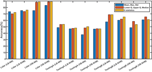
Among the proposed features, we observe that vector-based features outperform the length-based features in all cases, except for the “TestingB” of IAS-Lab. We hypothesize that changes in the illumination can lead to length-based features being more robust measures than vector-based features. Too much illumination can create a bleached-out image with insufficient contrast. In addition, we cannot see objects of interest in their true three-dimensionality if insufficient illumination is provided. Therefore, illumination variations can diminish the power of vector-based features.

In this work, we focused on a model-based gait recognition approach for flash lidar modality through an extensive joint correction of the estimated skeletons. Another possible approach can consist of filtering intensity and depth information and using the filtered data for pose estimation and gait recognition. But, we should note that the filtering of depth map in time-of-flight (TOF) cameras such as flash lidar is, in general, a computationally expensive process (Kim, Kim, and Yo-Sung 2013). Furthermore, due to the low resolution of both intensity and depth data of flash lidar, the effect of such filtering on the improvement of pose estimation and gait recognition is not clear.

The filtering mechanism presented here improves gait recognition by correcting missing and noisy skeleton joints in two steps. The two-step approach is vital, as it avoids the effect of noisy measurements in generating an initial prediction for the missing values in the first step. Besides, by adopting a robust smoothing filter in the second step, the negative effect of the remaining outliers and noisy prediction of the first step are diminished. However, there are cases that correction fails. Examples of such failures are shown in Figure 10. The filtering procedure can fail if a joint or a whole skeleton is missing over multiple consecutive frames. As the number of consecutive frames with a missing skeleton increases, the probability of failure rises. This is because the correction mechanism uses first-order polynomial fitting in the first step, which loses adequate support as the number of missing skeleton or missing joints increases. On the other hand, higher-order polynomial will over-smooth the final prediction, resulting in more false predictions. For a better imputation of missing values and correction of missing measurements, modeling the dynamics of the motion is also helpful. This is, in particular, essential in more realistic scenarios, where the dynamic of the motion such as the walking speed might change during motion. For such a direction of study, a larger collection of data from each subject would be required.

A major direction for future work calls for a dataset that consists of a larger population of subjects with a more diverse group of settings. This can be beneficial in multiple ways. First, it will open an avenue for training a deep pose estimation tool that generally requires a large and diverse collection of images. In the first step of the presented pipeline, we utilize OpenPose, a state-of-the-art pose estimation tool. As these tools are trained with images collected by optical cameras, their performance is adversely affected by the noisy imaging process of flash lidar cameras. With a large collection of flash lidar images, flash lidar-based deep pose models can be designed that can alleviate the performance of skeleton detection. Second, the availability of a large collection of flash lidar data paves the path for a well-designed optimization model to find relevant, yet interpretable features. In this work, we opt for anthropometric-based features to avoid the interpretability issue of a complex feature design. However, with a large data collection, there might be a need for a more distinct set of features to recognize a larger collection of the population considering the limitations of flash lidar modality.

Conclusion

In this work, we present an efficient pipeline to improve the application of flash lidar for the gait recognition problem. The main challenge is caused by the low quality and noisy imaging process of flash lidar. Such signal quality adversely affects the performance of state-of-the-art algorithms for skeleton detection. The detected skeletons from the collected sequences contain a considerable number of erroneous joint location measurements. Furthermore, detections for several skeleton joints are missing in many frames. Under the described scenario, a common practice involves removing noisy data. However, data elimination results in the loss of temporal information and renders identification impossible in numerous frames, which is not desirable for time-critical applications, such as with surveillance. To improve the quality of joint localization and to enhance gait recognition accuracy using flash lidar modality, we present GlidarPoly. GlidarPoly employs a filtering mechanism to correct faulty skeleton joint locations. We also present an automatic outlier detection method for applications where data elimination is not an issue. Furthermore, to incorporate motion dynamics after data correction, robust statistics are integrated that can effectively improve the performance of the designed features that only employ traditional feature moments over the gait cycles. The presented pipeline is appealing in terms of computational complexity, scalability, and a simple, yet effective design.

Disclosure statement

No potential conflict of interest was reported by the author(s).

Additional information

Funding

This work is supported in part by the Army Research Lab under Grant W911NF-20-1-0206.

Notes

1. A video presentation of before and after applying GlidarPoly is provided http://viva-lab.ece.virginia.edu/pages/projects/gaitrecognition.htmlhere

References

- Ahmed, F., P. Polash Paul, and M. L. Gavrilova. 2015. DTW-based kernel and rank-level fusion for 3D gait recognition using Kinect. The Visual Computer 31 (6–8):915–2514. doi:10.1007/s00371-015-1092-0.
- Ancong, W., W.-S. Zheng, and J.-H. Lai. 2017. Robust depth-based person re-identification. IEEE Transactions on Image Processing 26 (6):2588–603. doi:10.1109/TIP.2017.2675201.
- Araujo, R. M., G. Graña, and V. Andersson. 2013. “Towards skeleton biometric identification using the microsoft Kinect sensor.” In Proceedings of the 28th Annual ACM Symposium on Applied Computing, Coimbra, Portugal, 21–26. ACM.
- Babaee, M., L. Linwei, and G. Rigoll. 2018. “Gait recognition from incomplete gait cycle.” In 2018 25th IEEE International Conference on Image Processing (ICIP), Athens, Greece, 768–72. IEEE.
- Balazia, M., and K. N. Plataniotis. 2017. Human gait recognition from motion capture data in signature poses. IET Biometrics 6 (2):129–37. doi:10.1049/iet-bmt.2015.0072.
- Ball, A., D. Rye, F. Ramos, and M. Velonaki. 2012. “Unsupervised clustering of people from ‘skeleton’data.” In 2012 7th ACM/IEEE International Conference on Human-Robot Interaction (HRI), Boston Massachusetts USA, 225–26. IEEE.
- Batabyal, T., A. Vaccari, and S. T. Acton. 2015. “Ugrasp: A unified framework for activity recognition and person identification using graph signal processing.” In Image Processing (ICIP), 2015 IEEE International Conference, Quebec city, Canada, 3270–74. IEEE.
- Benedek, C., B. Gálai, B. Nagy, and Z. Jankó. 2018. “Lidar-based gait analysis and activity recognition in a 4d surveillance system.” IEEE Transactions on Circuits and Systems for Video Technology 28 (1):101–13.
- Cao, Z., T. Simon, S.-E. Wei, and Y. Sheikh. 2017. “Realtime multi-person 2d pose estimation using part affinity fields.“ In Proceedings of the IEEE conference on computer vision and pattern recognition, 7291–7299.
- Charalambous, C. P. 2014. Walking patterns of normal men. In Classic papers in orthopaedics, 393–95. London: Springer.
- Chattopadhyay, P., S. Sural, and J. Mukherjee. 2014. Frontal gait recognition from incomplete sequences using RGB-D camera.” IEEE Transactions on Information Forensics and Security. 9 (11):1843–56.
- Chi, W., J. Wang, and M. Q-H Meng. 2018. A gait recognition method for human following in service robots. IEEE Transactions on Systems, Man, and Cybernetics: Systems 48 (9):1429–40. doi:10.1109/TSMC.2017.2660547.
- Choi, S., J. Kim, W. Kim, and C. Kim. 2019. Skeleton-based gait recognition via robust frame-level matching. IEEE Transactions on Information Forensics and Security 14 (10):2577–92. doi:10.1109/TIFS.2019.2901823.
- Clark, R. A., K. J. Bower, B. F. Mentiplay, K. Paterson, and Y.-H. Pua. 2013. Concurrent validity of the Microsoft Kinect for assessment of spatiotemporal gait variables. Journal of Biomechanics 46 (15):2722–25. doi:10.1016/j.jbiomech.2013.08.011.
- Cleveland, W. S. 1979. Robust locally weighted regression and smoothing scatterplots. Journal of the American Statistical Association 74 (368):829–36. doi:10.1080/01621459.1979.10481038.
- Daugman, J. 2009. How iris recognition works. In The essential guide to image processing, 715–39. Amsterdam, Netherlands: Elsevier.
- Dikovski, B., G. Madjarov, and D. Gjorgjevikj. 2014. “Evaluation of different feature sets for gait recognition using skeletal data from Kinect.” In 2014 37th International Convention on Information and Communication Technology Electronics and Microelectronics (MIPRO), Opatija, Croatia, 1304–08. IEEE.
- Din, D., A. G. Silvia, and L. Rochester. 2016. Validation of an accelerometer to quantify a comprehensive battery of gait characteristics in healthy older adults and Parkinson’s disease: Toward clinical and at home use. IEEE Journal of Biomedical and Health Informatics 20 (3):838–47. doi:10.1109/JBHI.2015.2419317.
- Fankhauser, P., M. Bloesch, D. Rodriguez, R. Kaestner, M. Hutter, and R. Y. Siegwart. 2015. “Kinect v2 for mobile robot navigation: Evaluation and modeling.” In 2015 International Conference on Advanced Robotics (ICAR), Kadir Has University Cibali Confrence Center, Istanbul, Turkey, 388–94. IEEE.
- Gálai, B., and C. Benedek. 2015. “Feature selection for lidar-based gait recognition.” In Computational Intelligence for Multimedia Understanding (IWCIM), 2015 International Workshop, Prague, Czech Republic, 1–5. IEEE.
- Han, S. 2015. The influence of walking speed on gait patterns during upslope walking.” Journal of Medical Imaging and Health Informatics 5 (1):89–92.
- Han, J., and B. Bhanu. 2005. Individual recognition using gait energy image.” IEEE transactions on pattern analysis and machine intelligence 28 (2):316–22.
- Haque, A., A. Alahi, and L. Fei-Fei. 2016. “Recurrent attention models for depth-based person identification.” In Proceedings of the IEEE Conference on Computer Vision and Pattern Recognition, LAS VEGAS, Nevada, 1229–38.
- Horaud, R., M. Hansard, G. Evangelidis, and C. Ménier. 2016. An overview of depth cameras and range scanners based on time-of-flight technologies. Machine Vision and Applications 27 (7):1005–20. doi:10.1007/s00138-016-0784-4.
- Iwashita, Y., K. Uchino, and R. Kurazume. 2013. Gait-based person identification robust to changes in appearance. Sensors 13 (6):7884–901. doi:10.3390/s130607884.
- Jain, A. K., R. Bolle, and S. Pankanti. 2006. Biometrics: Personal identification in networked society, vol. 479. Berlin/Heidelberg, Germany: Springer Science & Business Media.
- Jang, C. H., C. S. Kim, K. C. Jo, and M. Sunwoo. 2017. Design factor optimization of 3D flash lidar sensor based on geometrical model for automated vehicle and advanced driver assistance system applications. International Journal of Automotive Technology 18 (1):147–56. doi:10.1007/s12239-017-0015-7.
- Kim, S.-Y., M. Kim, and H. Yo-Sung. 2013. Depth image filter for mixed and noisy pixel removal in RGB-D camera systems. IEEE Transactions on Consumer Electronics 59 (3):681–89. doi:10.1109/TCE.2013.6626256.
- Koide, K., and J. Miura. 2016. Identification of a specific person using color, height, and gait features for a person following robot. Robotics and Autonomous Systems 84 (84):76–87. doi:10.1016/j.robot.2016.07.004.
- Kovač, J., and P. Peer. 2014. Human skeleton model based dynamic features for walking speed invariant gait recognition. Mathematical Problems in Engineering 2014.
- Krzeszowski, T., A. Switonski, B. Kwolek, H. Josinski, and K. Wojciechowski. 2014. “DTW-based gait recognition from recovered 3-D joint angles and inter-ankle distance.” In International Conference on Computer Vision and Graphics, Warsaw, Poland, 356–63. Springer.
- Kumar, M. S., and R. Venkatesh Babu. 2012. “Human gait recognition using depth camera: A covariance based approach.” In Proceedings of the Eighth Indian Conference on Computer Vision, Graphics and Image Processing, Mumbai, India, 20. ACM.
- Liao, R., Y. Shiqi, A. Weizhi, and Y. Huang. 2020. A model-based gait recognition method with body pose and human prior knowledge. Pattern Recognition 98:107069. doi:10.1016/j.patcog.2019.107069.
- Liao, S., H. Yang, X. Zhu, and S. Z. Li. 2015. “Person re-identification by local maximal occurrence representation and metric learning.” In Proceedings of the IEEE conference on computer vision and pattern recognition, Boston, Massachusetts, 2197–206.
- Maltoni, D., D. Maio, A. K. Jain, and S. Prabhakar. 2009. Handbook of fingerprint recognition. Berlin/Heidelberg, Germany: Springer Science & Business Media.
- McCollough, E. 1893. Photographic topography. Industry: A Monthly Magazine Devoted to Science, Engineering and Mechanic Arts 54 (1):399–406.
- Munaro, M., A. Basso, A. Fossati, L. Van Gool, and E. Menegatti. 2014a. “3D reconstruction of freely moving persons for re-identification with a depth sensor.” In 2014 IEEE International Conference on Robotics and Automation (ICRA), Hong Kong, China, 4512–19. IEEE.
- Munaro, M., A. Fossati, A. Basso, E. Menegatti, and L. Van Gool. 2014b. One-shot person reidentification with a consumer depth camera. In Person re-identification, 161–81. London: Springer.
- Nasrin, S., A. G. Tamal Batabyal, N. K. Dhar, B. O. Familoni, K. M. Iftekharuddin, and S. T. Acton. 2019. “Glidar3DJ: A view-invariant gait identification via flash lidar data correction.“ In 2019 IEEE International Conference on Image Processing, Taipei taiwan, 2606–2610, IEEE.
- Oreifej, O., R. Mehran, and M. Shah. 2010. “Human identity recognition in aerial images.” In 2010 IEEE Computer Society Conference on Computer Vision and P attern R ecognition, San Francisco, CA, 709–16. IEEE.
- Pala, P., L. Seidenari, S. Berretti, and A. Del Bimbo. 2019. Enhanced skeleton and face 3d data for person re-identification from depth cameras. Computers & Graphics 79:69–80. doi:10.1016/j.cag.2019.01.003.
- Preis, J., M. Kessel, M. Werner, and C. Linnhoff-Popien. 2012. “Gait recognition with kinect.” In 1st international workshop on kinect in pervasive computing, New Castle, UK, 1–4.
- Rao, H., S. Wang, H. Xiping, M. Tan, Y. Guo, J. Cheng, X. Liu, and H. Bin. 2021. A self-supervised gait encoding approach with locality-awareness for 3d skeleton based person re-identification. IEEE Transactions on Pattern Analysis and Machine Intelligence 1–1. doi:10.1109/TPAMI.2021.3092833.
- Sadeghzadehyazdi, N., T. Batabyal, and S. T. Acton. 2021. Modeling spatiotemporal patterns of gait anomaly with a CNN-LSTM deep neural network. Expert Systems with Applications 185:115582. doi:10.1016/j.eswa.2021.115582.
- Schroff, F., D. Kalenichenko, and J. Philbin. 2015. “Facenet: A unified embedding for face recognition and clustering.” In Proceedings of the IEEE conference on computer vision and patternrecognition, Boston, Massachusetts, 815–23.
- Semwal, V. B., J. Singha, P. Kumari Sharma, A. Chauhan, and B. Behera. 2017. An optimized feature selection technique based on incremental feature analysis for bio-metric gait data classification. Multimedia Tools and Applications 76 (22):24457–75. doi:10.1007/s11042-016-4110-y.
- Sinha, A., K. Chakravarty, and B. Bhowmick. 2013. Person identification using skeleton information from kinect.” In Proceedings. International. Conference on Advances in Computer-Human Interactions 101–08.
- Smolik, M., V. Skala, and O. Nedved. 2016. “A comparative study of LOWESS and RBF approximations for visualization.” In International Conference on Computational Science and Its Applications, Beijing University of Posts and Telecommunications, Beijing, China, 405–19. Springer.
- Tang, J., J. Luo, T. Tjahjadi, and F. Guo. 2016. Robust arbitrary-view gait recognition based on 3d partial similarity matching. IEEE Transactions on Image Processing 26 (1):7–22. doi:10.1109/TIP.2016.2612823.
- Tukey, J. W. 1977. Exploratory data analysis, vol. 2. Reading, MA: Pearson.
- Xuequan, L., H. Chen, S.-K. Yeung, Z. Deng, and W. Chen. 2018. “Unsupervised articulated skeleton extraction from point set sequences captured by a single depth camera.” In Proceedings of the AAAI Conference on Artificial Intelligence, Hilton New Orleans Riverside, New Orleans, Louisiana, USA, vol. 32. 1.
- Xuequan, L., Z. Deng, J. Luo, W. Chen, S.-K. Yeung, and H. Ying. 2019. 3D articulated skeleton extraction using a single consumer-grade depth camera. Computer Vision and Image Understanding 188:102792. doi:10.1016/j.cviu.2019.102792.
- Yang, K., Y. Dou, L. Shaohe, F. Zhang, and Q. Lv. 2016. Relative distance features for gait recognition with Kinect. Journal of Visual Communication and Image R Epresentation 39:209–17. doi:10.1016/j.jvcir.2016.05.020.
- Zhang, Y., and L. Shutao 2011. “Gabor-LBP based region covariance descriptor for person re-identification.” In 2011 Sixth International Conference on Image and Graphics, Hefei, P.R.China, 368–71. IEEE.
- Zhao, L., L. Xuequan, M. Zhao, and M. Wang. 2021. “Classifying In-Place Gestures with End-to-End Point Cloud Learning.” In 2021 IEEE International Symposium on Mixed and Augmented Reality (ISMAR), Bari, Italy, 229–38. IEEE.
- Zheng, W., L. Lin, Z. Zhang, Y. Huang, and L. Wang. 2019. “Relational network for skeleton-based action recognition.” In 2019 IEEE International Conference on Multimedia and Expo (ICME), Shanghai, China, 826–31. IEEE.