Above-ground Biomass Wheat Estimation: Deep Learning with UAV-based RGB Images

ABSTRACT

Evaluation of biomass is essential in agriculture to delineate crop management practices, and this is usually done manually, which is time-consuming and destructive. This work proposes an artificial neural network and convolutional neural network to estimate the above-ground biomass (AGB) of wheat using visible spectrum images captured by an unmanned aerial vehicle. The utilized dataset has two Brazilian wheat types, called Parrudo and Toruk. Furthermore, the experimental area has variability in crop growth by varying the amount of nitrogen. To determine AGB, samples of plants were collected at three different crop growth stages, approximately a month apart, making our database spatial and temporal variability. We have shown the feasibility of developing a regression model using RGB images for biomass estimation for two wheat types. The best results for ANN were 489.5, 826.4, and 0.9056 for MAE, RMSE, and $R^2$, respectively. In CNN, MAE = 699.2, RMSE = 940.5, and $R^2$ = 0.9065. These results show high accuracy in estimation of biomass, and the $R^2$ shows good estimation and generalization capacity. The results demonstrate that our methodology can be used in precision agriculture to predict the spatial and temporal variability of AGB.

Introduction

Precision agriculture has grown in recent decades, and its importance for agricultural production in terms of productivity, environmental impact, and sustainability is vital. Biomass measurement, also known as above-ground biomass (AGB), is an important measure for yield and grain quality. Therefore, AGB is considered one of the most important crop parameters, and the correct estimation of AGB can help improve crop monitoring and yield prediction (Bendig et al. 2015; Brocks and Bareth 2018; Yue et al. 2017).

Traditionally, biomass measurement is done manually, which is time-consuming and destructive. In large areas, this measurement is impractical. To address these challenges, new technologies can be applied to cope with this task, such as unmanned aerial vehicle (UAV) for imaging and artificial intelligence for modeling. Despite limitations regarding its scalability for very large farms, UAV has been applied as an alternative for acquiring images with lower pixel size and higher temporal resolution than satellite (Ballesteros et al. 2018; Messinger, Asner, and Silman 2016).

Measuring biomass from imaging in order to improve precision agriculture has been demonstrated by several publications. Bendig et al. (2015) and Brocks and Bareth (2018) used a combination of selected vegetation indices (VIs) and plant height information to estimate the biomass of summer barley. According to Ballesteros et al. (2018), the estimation of onion crop biomass from high-resolution imaging obtained with UAV was based on green canopy cover, crop height and canopy volume as the predictor variables. Messinger, Asner, and Silman (2016) investigated the use of UAVs to measure above-ground carbon density in forests to replace expensive or labor-intensive inventory methods.

Several works have been published in which an attempt is made to estimate wheat biomass from images (Fu et al. 2014; Gaso, Berger, and Ciganda 2019; Yue et al. 2017), investigating several regression methods. Yue et al. (2017) proposed the estimation of wheat biomass using linear models, hyperspectral sensing, and several vegetation indices. Fu et al. (2014) have used the vegetation index NVDI to calculate wheat biomass. They have shown a linear relationship between NDVI and measured biomass. However, the results are presented with only one manual collected sample of biomass, limiting the aspects of temporal variability of the biomass. Furthermore, contrary to their research, given the need for a special camera or a specific sensor, we do not use VIs, multispectral images, or the NDVI in our work. Based on this, we investigate the possibility of using only RGB images. Furthermore, we have collected samples of biomass from three different stages of wheat development, which provides a more reliable model.

In precision agriculture, artificial intelligence (AI) is typically used to classify diseases like the work found in Brahimi, Boukhalfa, and Moussaoui (2017), where a convolution neural network (CNN) is used to classify nine tomato diseases. In that work, they compare two well-known architectures of CNN with $99\mathrm{\%}$ of accuracy. Zounemat-Kermani (2014) proposed predicting the value of chlorophyll, a parameter for estimating primary productivity, biomass, and so forth. They have used linear regression and ANN feed-forward networks using the PCA as the network’s data input. Wang et al. (2016) investigated the applicability of the Random Forest regression algorithm with VIs to remotely estimate (satellite) wheat biomass.

Gopal and Bhargavi (2019) proposed the use of other kinds of features for machine learning in Wheat Biomass estimation: the number of fertilizers, cumulative rainfall, among others. Whereas in our work, only images are used for crop yield prediction. Ighalo, Igwegbe, and Adeniyi (2021) utilized a multi-layer perceptron artificial neural network (MLP-ANN) model to predict the higher heating values (HHV) of biomass based on 210 lines of combined proximate and ultimate analysis data. In a recent survey on deep learning in agriculture (Kamilaris and Prenafeta-Boldú 2018), 48 works have been reported on agriculture applications, such as identification of weeds, fruits counting, and crop-type classification. Most applications that use deep learning in the literature are for object classification. Although there are some previous works with AI applied to agriculture precision, estimation of wheat biomass and yield prediction using deep learning is still a largely unexplored field.

Motivated by the advances in artificial intelligence and the importance of automatic biomass estimation for agriculture precision, we propose in this work an application for estimation of wheat biomass based on RGB images acquired by a UAV using two paradigms of deep learning. The first one is a traditional fully connected artificial neural network (ANN), and the other one is a convolutional neural network (CNN). Despite the advance of CNNs and their architectures, and thus the availability of various public libraries with competent CNN implementations – as shown by Khan et al. (2019) – we have implemented our CNN architecture. In so doing, we have control for tuning the hyperparameters and finding the most suitable CNN for our task. In addition, we have compared the results using a well-known ANN network with a CNN.

The contributions of this work are summarized as follows: (a) A comparison of two regression models for estimation of wheat biomass using Artificial Intelligence; (b) The use of two wheat genotypes for training the AI models; (c) The set of data with spatial and temporal variability that provides a more realistic scenario. The dataset is available (Schreiber, Amorim, and Parraga 2020); (d) The feasibility of developing a regression model using visible imaging (RGB), which has the advantage of lower cost for real practice in agriculture when compared to hyperspectral cameras.

Material and Methods

This section describes the data acquisition, the models, the preprocessing of data, and the metrics to model evaluation. The experimental wheat crop field is presented, along with image acquisition and manual biomass measurements throughout the crop development.

Data Acquisition

For this work, an experimental wheat crop field area of 60 m × 20 m was used. The experiments were conducted at the Agriculture Experimental farm located in the south of Brazil, from May to October in 2018. The study area contains several 2.5 m × 1 m rectangular parcels, which are referred to as plots, which hold two Brazilians wheat varieties.

The genotypes used were TBIO Toruk and BRS Parrudo (48 Toruk plots and 40 Parrudo plot). Variability in the crops growth was created for all test areas, where each one received a varying quantity of nitrogen. Different nitrogen (N) rates were chosen to generate crop growth variability, to evaluate the response of biomass and grain yield to N availability, which we called spatial variability. The database consists of images captured by unmanned aerial vehicles (UAVs) and biomass manual measured to develop the estimation models. A workflow for the database acquisition can be seen in Figure 1.

Figure 1. Workflow for data acquisition.

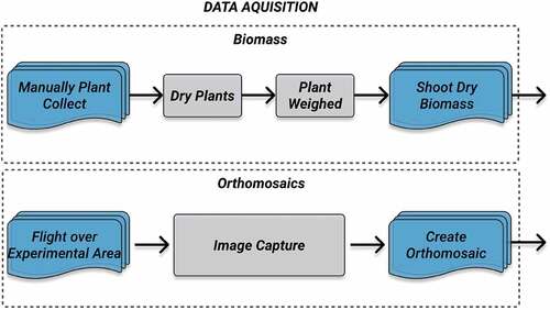
Biomass Measurement: To train a network and develop a biomass estimation model, we collected real biomass to create a ground-truth. This step is done manually and in a destructive way, as follows. Shoot dry biomass was determined at three growth stages: the stage of six fully expanded leaves, referred herein as V6, three nodes, and at flowering by the collecting of plants in an area of 0.27 m² for each plot. This was done to create a temporal variability. The plants collected were oven-dried at 65°C until constant weight and weighed. Then the weight is extrapolated for kilograms/hectare (kg/ha). The average biomass measurements are presented by stage in Table 1.

Table 1. Biomass average in kg/ha by stage.

	Parrudo	Toruk	Both Cultivars
V6	683.5	529.9	606.7
Three nodes	2147.4	1993.6	2070.5
Flowering	6769.4	5728.4	6248.9
Average of all stages	3200.1	2750.6	2975.4

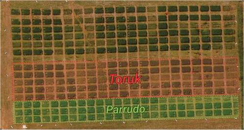
UAV-based Data Collection: The images used in this work were acquired at the height of 50 m above ground using a camera coupled to a DJI Matrice 100 Quadcopter. This camera is a single-channel DJI X3 Visible (RGB), with 12MB resolution and 8-bit pixel depth. For agriculture acquisition, the recommended frontal overlap should be at least 80%, and the side overlap should be at least 70%. The resulting pixel size for the RGB images is 2.14 cm${ }^2$/px. A total of 30 individual images were captured by the UAV using these parameters. Post-processing of the acquired images included georeferencing and mosaicking using photogrammetric software (Agisoft 2018), where a large set of overlapping images are post-processed to produce a single global orthoimage. Several ground control points were used around the experimental crop field and their geographic coordinates were evaluated using a high precision RTK GPS. The use of ground control points allows the alignment of orthoimages obtained from different dates by the generation of a georeferenced orthomosaic image. The final orthomosaic image can be seen in Figure 2, acquired on August 28, 2018.

Figure 2. Orthomosaic image showing the experimental area (crop field of 60 m × 20 m), with two types of winter Brazilians wheat. Toruk plots are highlighted by the red rectangle and the Parrudo plots are highlighted by the green rectangle (acquired on August 28, 2018).

Our UAV’s three stages of growth were captured on the dates described in Table 2. It is at these stages that the biomass collection (ground truth) occurs.

Table 2. Crop growth stage, image acquisition dates and number of plot samples in each date.

		Number Plot Samples
Crop growth stage	UAV acquisition	Toruk	Parrudo
V6	July, 2018	40	48
Three nodes	August, 2018	40	48
Flowering	September, 2018	40	48

Preprocessing Data

To feed and train ANN and CNN, the first step is to segment the plots from the orthomosaic presented in Figure 2. In this work, data from the different plots were obtained using QGIS 3 (Team et al. 2018). Each estimation method does not have the same data entry, so each one has its data segmentation and data input strategy, as described in the sequence.

ANN: From the orthomosaic, regions of interest (ROI) were manually delineated from each plot of the orthomosaic, as shown by the red dots in Figure 3a. The ROIs were selected in a way that excluded pixels with soil exposed. Then from each ROI, an average of pixels was performed in the three RGB channels. This triplet of average was used as the input data to train our proposed ANN architecture.

Figure 3. (a) Plot ROI delineation example for the creation of the average pixels array for the entry of ANN. (b) Example of wheat plot image input for CNN.

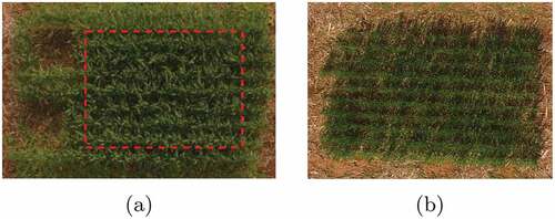
CNN: For the CNN approach, each plot was segmented using a mask with regular size. This mask was used to provide the entry images with the standard size (Long, Shelhamer, and Darrell 2015) and is the same for the three different dates and development stages of the wheat.

After segmentation of 88 plots for each day of Biomass manual cutoff, according to Table 2, we obtained 264 RGB images with 158 × 110 pixels. Figure 3b shows an example of this segmented plot.

Proposed Models

The two architectures proposed in this work, ANN and CNN, were implemented using Python 3.6 (Van Rossum and Drake 1995), with the Keras Library (Chollet et al. 2015) and scikit-learn (Pedregosa et al. 2011). These methods have several advantages, such as the ability to capture the nonlinear relation among data. Below, we present the details of each architecture implemented.

ANN

The ANN structure can be divided into three parts: the input layer, the hidden layers, and the output layer. The input layer has the numeric values of the inputs, which describe the data being modeled. Figure 4 shows the global structure proposed in this work that provided the best results for biomass estimation. The model of our ANN is

Figure 4. ANN Model Proposed.

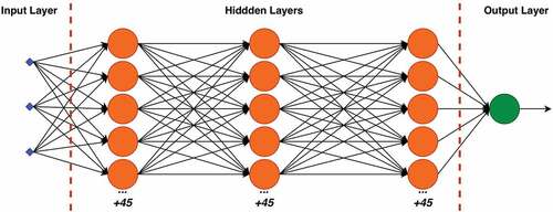
• The input layer has three input neurons, the average of pixel values for each of the three channels (R, G and B).

• There are three hidden layers connected, each layer with 50 neurons with ReLU activation function.

• The output layer has one neuron with a linear activation function.

A data normalization step is performed in the output of each hidden layer to improve the learning rate. Next, a dropout layer is used, responsible for random deactivation of a percentage of the neurons during the training. The percentage values were 20% for each hidden layer. The dropout technique is used to avoid overtraining of the network (Nielsen 2015). Finally, the number of training epochs, batch size, optimizer, learning rate, loss function, and metrics are given in Section 3.1.

CNN

Convolution neural network is a paradigm of deep learning that comprises in its structure the process of feature learning, by applying several kernels for feature extraction, and a classification with fully connected layers. Therefore, a CNN has the ability of learning discriminant features directly from images, video, text, or sound (Gavrilov et al. 2018).

CNN layers consist of an input and an output, with multiple hidden layers between them. The hidden layers mainly include three types, namely convolutional layer, pooling layer, and fully connected layers (Krizhevsky, Sutskever, and Hinton 2017). Each layer of a CNN has $n$ filters containing a three-dimensional array. The input layer will contain the values of the raw pixels of the images.

We divide the structure for CNN into two parts: the feature extraction and the fully connected layers. The architecture proposed for the first one can be seen in Figure 5, where the hyperparameters chosen for Feature Extraction of the CNN used in this work are shown. The details of the feature extraction implemented are

• Convolution operation is performed in the input image with a kernel that seeks for features. In this case, we have used 16 filters;

• A down sampling is done in this group of features using max-pooling with parameter 2, that is, we reduce the size of the image by half;

• Another convolution operation is done with 32 new filters, creating a new group of features map;

• A down sampling is performed on this new group of characteristics using max-pooling again with parameter 2;

• In the last layer of convolution, convolution operation was done using 64 filters to create the features maps;

• In the last down sampling, max-pooling is used again with parameter 2;

• In the last step of the feature extraction layer, a flattening is made, which takes each feature map and creates an array of 15808 values.

Figure 5. CNN model proposed.

After the feature extraction, the flattening array feeds fully connected layers to perform the final estimation model, as previously said. These layers are extremely similar to the ANN shown in Figure 4. The number of training epochs, the steps per epoch, optimizer, learning rate, loss function, and metrics can be seen in Section 3.1.

Experiment Settings

In the training process, different images at different periods were all pooled together as inputs to find a general model. To train both deep learning networks, ANN and CNN, it is necessary to separate the database into training and testing data sets. To train and measure the performance, we have used cross-validation with the k-fold method, which is a technique that divides data samples into a training and a test set and has an excellent performance to overcome overfitting (Santos et al. 2018).

For the cross-validation, we have used k = 10, where the whole database is divided into 10 parts or folds. All k folds are randomly chosen. One fold is left out for testing, and the other nine folds for training. As we have used k = 10, it means that 10% of the entire database was used for testing, that is, 27 plot images.

For the training, 30 different seeds were used to create a random number generator, which means that we have trained the networks 30 times, altering the data order. So, each network was trained for each seed exclusively, and this result generates a model; at the end of this process, we have 30 ANN and 30 CNN models. In short, the idea is to validate that regardless of the test and training set, the model can converge.

Metrics for Model Evaluation

To evaluate each network architecture’s performance, evaluate each regression model, and define a standard of comparison, we established the use of three metrics. These metrics are root-mean-square error (RMSE), mean absolute error (MAE) and coefficient of determination ($R^2$) (Willmott and Matsuura 2005). MAE and RMSE metrics are the most common ones to evaluate regression and have the same measure of magnitude as the input data, such as kilograms per hectare (kg/ha). Results are presented for each metric, showing their best values for all sets of the training process, with the mean value and the standard deviation for each one.

For all evaluation equations from Equations (1)(1) $MAE=\frac{1}{n}\sum _{j=1}^n|y_j-{\hat{y}}_j|$(1) to (3), $n$ is the total number of samples, $y_j$ is the measured value (ground truth value), ${\hat{y}}_j$ is the predicted value, and $\bar{y}$ is the mean of the measured data.

Mean absolute error (MAE): It is the mean of the absolute difference between the predicted values and the observed (residual) value, where all individual differences are weighted equally on average (Willmott and Matsuura 2005). Its value can range from 0 to $\mathrm{\infty }$, where smaller values indicate that the predicted values are closer to the measured values.

(1) $MAE=\frac{1}{n}\sum _{j=1}^n|y_j-{\hat{y}}_j|$(1)

Root mean square error (RMSE): The RMSE is the sample standard deviation of the differences between the predicted values and the measured (residual) values (Willmott and Matsuura 2005). The RMSE, different from the MAE, penalizes the larger differences more strongly (Chai and Draxler 2014).

(2) $RMSE=\sqrt{\frac{1}{n}\sum _{j=1}^n{(y_j-{\hat{y}}_j)}^2}$(2)

Coefficient of determination ($R^2$): It is a statistical measure of how well regression forecasts approximate actual data points. This value can be in percentage, providing how much the model can explain the observed values. Its value can range from 0 to 1, and the higher the $R^2$, the better the data fits the model (Montgomery and Runger 2010).

(3) $R^2=\frac{\sum _{j=1}^n{({\hat{y}}_j-\bar{y})}^2}{\sum _{j=1}^n{({\hat{y}}_j-\bar{y})}^2+\sum _{j=1}^n{(y_j-\hat{y})}^2}$(3)

Table 3 summarizes the range for each metric used and the target value for best accuracy.

Table 3. Metrics used for regression evaluation.

Metric	Min.	Max.	Obs.
Mean absolute error (MAE)	0	$\mathrm{\infty }$	Smaller better
Root mean square error (RMSE)	0	$\mathrm{\infty }$	Smaller better
Coefficient of determination ($R^2$)	0	1	Higher better

Results and Discussions

The results are presented in three parts. First, we present the hyperparameters that we implemented for the proposed application to estimate the wheat biomass. Second, we show the numerical results applied to the real data described in the methodology section. In the last part, we show the biomass map for each method. It is worth noting that each section has a brief discussion of the results obtained.

Hyperparameters Tuning

The hyperparameter tuning was performed thanks to the Hyperopt library (Bergstra, Yamins, and Cox 2013). This library helped to reduce the size of the tests. In Table 4, we briefly present each hyperparameter chosen for ANN and CNN.

Table 4. Hyperparameters for both models.

	Epochs	Steps per Epoch	Batch Size	Optimizer	Learning Rate	Loss Function	Metrics
ANN	1000	–	4096	Adadelta	0.1	MSE	$R^2$, RMSE, MAE
CNN	50	30	–	SGD	0.002	MSE	$R^2$, RMSE, MAE

Numerical Results

Table 5 presents the numerical results found for the ANN and CNN networks after training 30 times. The first row gives the average and standard deviation for all the 30 trainings. We also show the best result for each metric in the second row.

Table 5. Average, standard deviation and the best result for both ANN and CNN methods.

		MAE (kg/ha)	RMSE (kg/ha)	$R^2$
ANN	Average	506.7 $\pm$ 6.9	871.7 $\pm$ 14.3	0.8930 $\pm$ 0.006
	Best result	489.5	826.4	0.9056
CNN	Average	786.0 $\pm$ 27.6	1020.22 $\pm$ 37.3	0.9013 $\pm$ 0.005
	Best result	699.2	940.5	0.9065

As we can see, the models were well-adjusted since we found a high $R^2$ value for both networks. ANN performed better for MAE and RMSE errors in kg/ha. The results in Table 5 are presented together for all stages. Suppose we consider the biomass average for all stages and both cultivars. In that case, the mean value is $2975.35\mathrm{k}\mathrm{g}/\mathrm{h}\mathrm{a}$ (see Table 1), resulting in a percentage MAE error of approximately $16\mathrm{\%}$, and a percentage RMSE of $27.7\mathrm{\%}$ for the ANN network. For the CNN, it resulted in a percentage MAE error of approximately $23\mathrm{\%}$ and a percentage RMSE $31.6\mathrm{\%}$

We also presented the outcome by stages to better understand these results, which can be important for the agriculture practice. The graphics comparing the real value of Biomass and the predicted one are presented in Figures 6 a and b. The red lines in these figures represent the real value, and the green lines the prediction for each model. The outcome is very promising.

Figure 6. Real Biomass and Biomass Estimation by (a) ANN with an error range, (b) by CNN with an error range.

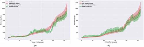
We compare the estimation results for the ANN and CNN architectures by samples. We can see that in the initial samples, the networks performed more accurately when compared to the final stages. However, both had a higher error; this can be explained by the fact that the wheat has flowered in the last samples (taken during the flowering stage), and the color pattern starts to change. In this case, it is ready to harvest the plantation. In addition, we can also see the CNN generalized the biomass growth better than the ANN.

Biomass Map

For a visual comparison, we also created a Biomass Map, which helps understand and presenting the results. The idea is to create a sort of heat map, where the intensity of the color will represent the predicted biomass for each model. Of course, each algorithm needs to generate this map differently, but briefly speaking, the idea is to use the whole orthomosaic as input for the algorithms and create a new image for each model output.

The ANN Biomass Maps are in Figure 7a,b and c for each crop stage. These Biomass maps were created by taking each pixel of the original images and putting in the ANN model’s entry for estimating the biomass and creating these maps. For both models, the colors indicate the Biomass in $\mathrm{k}\mathrm{g}/\mathrm{h}\mathrm{a}$.

Figure 7. Biomass Map for ANN in the (a) V6 crop stage (b) Three nodes crop stage (c) Flowering crop stage. The colors indicate the Biomass in $\mathrm{k}\mathrm{g}/\mathrm{h}\mathrm{a}$.

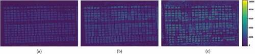
The CNN Biomass Maps are in Figure 8a, b and c for each crop stage. Unlike ANN, these Biomass maps were created by using each wheat plot in the original image, and this whole piece became a single biomass value, so it seems to have a lower resolution and could not be applied to the corners of the image. However, using a few meters as input in hectares makes this difference hardly noticeable. As said before, the colors indicate the Biomass in $\mathrm{k}\mathrm{g}/\mathrm{h}\mathrm{a}$.

Figure 8. Biomass Map for CNN in the (a) V6 crop stage. (b) three nodes crop stage. and (c) flowering crop stage. The colors indicates the biomass in $\mathrm{k}\mathrm{g}/\mathrm{h}\mathrm{a}$.

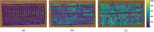
The comparison of the biomass maps between the algorithms is a bit difficult. This is because each map has characteristics that stand out between them. For example, for ANN, the soil was clearly highlighted when comparing the plots, allowing a quick observation of where has or not wheat planted or where there might be a problem during growth. However, during the stages, the CNN biomass maps better differentiate the value of growth over time.

Conclusions and Future Work

This study has proposed a deep learning approach to build a model for estimation of wheat biomass. To achieve that, we implemented two paradigms, ANN and CNN, with color images acquired by a UAV. The obtained results demonstrated the feasibility of the proposed approach to model shoot biomass for Brazilian wheat varieties. Furthermore, our results show that both deep models provided good results and are promising tools for agricultural practice. We have observed that both ANN and CNN performed similarly for practical purposes, although ANN can be more convenient, since it has a simpler structure.

Our experiments have also validated a different, and less costly, approach to automatic biomass estimation, since we have used only RGB images, thus not requiring cameras that capture multi-spectral images. To share with all interested parties who wish to work with our data, the access to the Brazilian Wheat Dataset (Schreiber, Amorim, and Parraga 2020) developed during this work is one of its contributions. This dataset has more than 9 thousand unique data and more than 190 MB of images.

As future work, we plan to investigate using more input parameters and images to improve the results, develop a comparison between ready and validated models, and compare hyperspectral data and images with RGB.

Acknowledgments

Authors would like to thank Fapergs (the Brazilian Foundation for Science and Technology) for funding the project under grant 16/2551-0000524-9 and CAPES – Coordination of Improvement of Personal Higher Education (Brazil).

Disclosure Statement

No potential conflict of interest was reported by the author(s).

Additional information

Funding

This work was supported by the FAPERGS [16/2551-0000524-9].

References

- Agisoft, L. 2018. Agisoft photoscan user manual. Professional edition, version 1.4, 1, 124.
- Ballesteros, R., J. F. Ortega, D. Hernandez, and M. A. Moreno. 2018. Onion biomass monitoring using UAV-based RGB imaging. Precision Agriculture 19 (5):840–2557.
- Bendig, J., K. Yu, H. Aasen, A. Bolten, S. Bennertz, J. Broscheit, M. L. Gnyp, and G. Bareth. 2015. Combining UAV-based plant height from crop surface models, visible, and near infrared vegetation indices for biomass monitoring in barley. International Journal of Applied Earth Observation and Geoinformation 39:79–87.
- Bergstra, J., D. Yamins, and D. Cox. 2013. Making a science of model search: Hyperparameter optimization in hundreds of dimensions for vision architectures. International Conference on Machine Learning 28: 115–23.
- Brahimi, M., K. Boukhalfa, and A. Moussaoui. 2017. Deep learning for tomato diseases: Classification and symptoms visualization. Applied Artificial Intelligence 31 (4):299–315.
- Brocks, S., and G. Bareth. 2018. Estimating barley biomass with crop surface models from oblique RGB imagery. Remote Sensing 10 (2):268.
- Chai, T., and R. R. Draxler. 2014. Root mean square error (RMSE) or mean absolute error (MAE)? Geoscientific Model Development Discussions 7 (1):1525–34.
- Chollet, F. et al. 2015. Keras: Deep learning library for theano and tensorflow. https://keras.io/getting_started/faq/#how-should-i-cite-keras
- Fu, Y., G. Yang, J. Wang, X. Song, and H. Feng. 2014. Winter wheat biomass estimation based on spectral indices, band depth analysis and partial least squares regression using hyperspectral measurements. Computers and Electronics in Agriculture 100:51–59.
- Gaso, D. V., A. G. Berger, and V. S. Ciganda. 2019. Predicting wheat grain yield and spatial variability at field scale using a simple regression or a crop model in conjunction with Landsat images. Computers and Electronics in Agriculture 159:75–83.
- Gavrilov, A., A. Jordache, M. Vasdani, and J. Deng. 2018. Convolutional neural networks: Estimating relations in the ising model on overfitting. 2018 IEEE 17th International Conference on Cognitive Informatics & Cognitive Computing (ICCI*CC). Berkeley, CA, USA. doi:10.1109/ICCI-CC.2018.8482067.
- Gopal, M., and Bhargavi. 2019. Performance evaluation of best feature subsets for crop yield prediction using machine learning algorithms. Applied Artificial Intelligence 33 (7):621–42.
- Ighalo, J. O., C. A. Igwegbe, and A. G. Adeniyi. 2021. Multi-layer perceptron artificial neural network (MLP-ANN) prediction of biomass higher heating value (hhv) using combined biomass proximate and ultimate analysis data. Modeling Earth Systems and Environment 7 3 1–15.
- Kamilaris, A., and F. X. Prenafeta-Boldú. 2018. Deep learning in agriculture: A survey. Computers and Electronics in Agriculture 147:70–90.
- Khan, A., A. Sohail, U. Zahoora, and A. S. Qureshi. 2019. A survey of the recent architectures of deep convolutional neural networks. CoRR, abs/1901.06032.
- Krizhevsky, A., I. Sutskever, and G. E. Hinton. 2017. ImageNet classification with deep convolutional neural networks (6th ed.). Communications of the ACM 60(6):84–90.
- Long, J., E. Shelhamer, and T. Darrell. 2015. Fully convolutional networks for semantic segmentation. 2015 IEEE Conference on Computer Vision and Pattern Recognition (CVPR), Boston, MA, USA.
- Messinger, M., G. Asner, and M. Silman. 2016. Rapid assessments of Amazon forest structure and biomass using small unmanned aerial systems. Remote Sensing 8 (8):615.
- Montgomery, D. C., and G. C. Runger. 2010. Applied statistics and probability for engineers. Nova Jersey, EUA.: John Wiley & Sons.
- Nielsen, M. A. 2015. Neural networks and deep learning, vol. 25. San Francisco, CA, USA: Determination press.
- Pedregosa, F., G. Varoquaux, A. Gramfort, V. Michel, B. Thirion, O. Grisel, M. Blondel, P. Prettenhofer, R. Weiss, V. Dubourg, et al. 2011. Scikit-learn: Machine learning in python. Journal of Machine Learning Research 12 (Oct):2825–30.
- QGIS Development Team 2018. Qgis geographic information system. open source geospatial foundation project. http://qgis.osgeo.org.
- Santos, M. S., J. P. Soares, P. H. Abreu, H. Araujo, and J. Santos. 2018. Cross- validation for imbalanced datasets: Avoiding overoptimistic and overfitting approaches [research frontier]. IEEE Computational Intelligence Magazine 13 (4):59–76.
- Schreiber, L. V., J. G. A. Amorim, and A. Parraga. 2020. (2020) Brazilian wheat dataset. Mendeley Data V1. doi:10.17632/3ntkg88d4d.1
- Van Rossum, G., and F. L. Drake Jr. 1995. Python tutorial. Amsterdam, Netherlands: Centrum voor Wiskunde en Informatica.
- Wang, L., X. Zhou, X. Zhu, Z. Dong, and W. Guo. 2016. Estimation of biomass in wheat using random forest regression algorithm and remote sensing data. The Crop Journal 4 (3):212–19.
- Willmott, C., and K. Matsuura. 2005. Advantages of the mean absolute error (MAE) over the root mean square error (RMSE) in assessing average model performance. Climate R Esearch 30:79–82.
- Yue, J., G. Yang, C. Li, Z. Li, Y. Wang, H. Feng, and B. Xu. 2017. Estimation of winter wheat above-ground biomass using unmanned aerial vehicle-based snapshot hyperspectral sensor and crop height improved models. Remote Sensing 9 (7):708.
- Zounemat-Kermani, M. 2014. Principal component analysis (pca) for estimating chlorophyll concentration using forward and generalized regression neural networks. Applied Artificial Intelligence 28 (1):16–29.