Research on Multi-side Joint Industrial Parts Inspection Based on Model Fusion

ABSTRACT

Rapid identification of many industrial material parts is the key to effectively improving the efficiency of the industrial production process and intelligent warehousing. Accurate identification of both similar and special parts is an important problem. In this paper, a multi-side joint industrial part recognition method based on model fusion learning is proposed. A multi-channel visual acquisition system is designed to construct a fast industrial part data set with time and space consistency. Two joint identification methods for multi-side acquisition are proposed, and the classification results are fused to improve the model’s accuracy and solve the classification problem for similar parts. The experimental results show that compared with the traditional model, the prediction accuracy of the multi-channel multi-input model proposed in this paper is improved by approximately 6%, and the accuracy of the single-channel multi-input model is improved by approximately 10%. The accuracy of part recognition is far better than that of the traditional model, and it therefore provides a new strategy for the rapid training and recognition of industri-al parts in intelligent storage.

Introduction

Against the background of Industry 4.0, the scale and mode of production have undergone significant changes. There are thousands of parts in the industrial production warehouse system, and this magnitude requires quick and accurate procurement of the necessary parts. First, manual operation is slow. Second, in large-scale industrial automation products, the probability of equipment part failure remains high and requires timely replacement. Rapid replacement of damaged parts can maintain higher productivity. For ease of use, the concept of intelligent warehousing is proposed to find the faulty parts quickly. Its purpose is to scientifically and effectively manage existing warehouse parts and raw production materials. At present, the two-dimensional code or bar code identification methods are the general way to quickly find stored parts in industrial production. However, it is challenging to perform two-dimensional code identification for small-batch, abnormal appearance parts. Most existing methods for finding parts in industrial output use the two-dimensional code identification method, which can perform quick searches by scanning the two-dimensional code. Still, it is challenging to perform two-dimensional code identification for small-batch parts with abnormal appearances. The current method used to search for these parts is to use experienced workers to identify the part type, who then locate the part in the warehouse to replace them. This solution to this problem heavily depends on very high requirements for worker experience. It is not a general solution since it is not fast or accurate and easily leads to errors.

In most cases, it cannot effectively solve the problem and cannot meet its requirements for speed and accuracy. The use of automated methods for identifying special-shaped parts is a problem that involves classifying and recognizing special objects. The essence of the problem is to identify parts using image features to achieve rapid search and retrieval of parts.

In recent years, some scholars and experts have proposed solving problems in the production process of industry and other fields based on machine learning and visual algorithms. The adaptive Scale-invariant feature transform algorithm is used for face recognition under an uncontrolled light source, which solves a difficulty for face recognition under a change in solid light (Meriama and Mohamed 2018) . The FCM clustering method is used to classify the color and pattern elements of printed fabric, and then Hough transform is used to segment the pattern image in duplicate mode (Chung, Jeffrey and Kuo 2016). Several appropriate processing areas in the picture are selected, and then for each area, the lane features are extracted through preprocessing, edge detection, and Hough change. The experimental results show that this method has good real-time performance and high reliability (Li, Zhang, and Bian 2004) . In addition, the SVM is also used to predict the stability of underground mine pillars (Li et al. 2011) and is based on the traditional image feature extraction methods to solve practical problems in different fields.

Traditional methods for solving the problem primarily rely on the manual extraction of the data set’s characteristics or the extraction of the shape characteristics based on the artificially designed algorithm. Supposing the traditional method is used to solve the part recognition problem, there will be significant errors if different shooting angles are used to identify the parts. If the parts are contaminated with oil and therefore damaged, it will also significantly impact part color recognition. Due to the complex features found in hundreds of parts, the similarities in parts categories and the differences outside categories are large. These traditional methods need improved flexibility when managing large data sets and problems.

With the development of computer vision technology in recent years, object recognition, detection, and tracking based on deep learning have made progress. With the development of the theory of deep learning (LeCun, Bengio, and Hinton 2015) and the improvement of computational power, the concept of the neural network has been proposed by using the pioneer of the neural network, Lenet (LeCun et al. 1998), as a starting point. AlexNet (Krizhevsky, Sutskever, and Hinton 2012) successfully uses deep network. VGG (Russakovsky et al. 2015) proposed that convolutions of different shapes extract different features. GoogleNet (Ioffe and Szegedy 2015; Szegedy et al. 2015, 2016, 2016) proposed a variety of convolution operations with deeper layers and wider widths. Res-Net (Kaiming et al. 2016) and DenseNet (Huang, Liu, and Laurens 2017) both used the idea of residual transfer. DenseNet is more concise and uses the concept of feature reuse, which improves the accuracy of object recognition. Deep learning methods have also begun to be applied to solve practical problems. For example, the combination of industrial 4.0 and deep learning has accelerated the development of the industrial field. For the management of intelligent buildings, deep learning and the Internet of Things are used to achieve efficient management (Elsisi et al. 2021) . Various aspects of life have gradually begun to apply deep learning technology. Aiming at the problem of garbage classification, a garbage classification method based on transfer learning is proposed. The results show that the model has good performance, high accuracy, and can correctly classify garbage (Cao and Wei 2020) . Aiming at the classification of diseases, deep learning is used to classify various types of diseases and help doctors diagnose patients better (Demizio and Bernstein 2019; Roy et al. 2020; Shah, Ana, and Jens 2020; Xiaojun and Haibo 2019;) . In the fault classification and diagnosis of industrial machines, great progress has been made in fault diagnosis of induction motors using multi-modal neural networks and fault diagnosis of diesel engines using attention-based convolutional neural networks (Fu et al. 2020; Xie et al. 2020) . In addition, wavelet transforms preprocessing and deep convolution neural network are used to detect milling chatter (Sener et al. 2021) .

It is of great significance to study parts classification in industrial scenes, but there is no available data set for part recognition research. When collecting the part data set, it was found that the data has certain characteristics because most parts are regular geo-metric shapes. Still, a small number of shapes do not meet this condition and are unregular. To accurately classify industrial storage parts, it is necessary to solve the classification problem for complex or un-regular shapes, which is decomposed into three issues that must be solved:

1. The problem of inconsistent part positions in recognition: t. The geometric shape of parts must be mathematically calculated when the traditional method identifies the parts. When the camera deviates or the relative position of the parts changes, the calculation parameters are affected.

2. The problem of multiple feature surfaces. It is necessary to collect multi-angle data to ensure that the data to be identified can be identified at any acquisition angle. When collecting image data for polyhedron parts, the parts must be flipped several times so that the shape of the parts at all observed angles is collected.

3. The problem of similarity. Due to similarities be-tween parts, the same image data correspond to different label data after collection. Since there are multiple similar specifications for parts in practical problems, the side image features collected from some observed angles of the parts are consistent. The traditional method cannot solve such classification problems. In the learning process for similar samples, the neural network will also be unable to accurately identify similar data samples because of multiple label mapping problems. It is uncertain about identifying the similar data samples accurately. Due to a good degree of discrimination in training, the premise of accurate identification is that there is a good degree of discrimination in training. The accuracy of the detection of similar shape parts will therefore reduce.

In the analysis of the above problems, it is found that the third point is the key to solving the classification problem for many sets of parts because single angle fixed camera shooting cannot show all the sur-face features of the parts at once, and only one-sided features can therefore be collected. For a variety of different types of parts with consistent single-side features, single-side detection, which is realized by the traditional single-channel input model, struggles when performing part detection. In this case, the part detection accuracy will decrease. Given the above problems, this paper first designs and implements a multi-channel part image data acquisition system and constructs a space-time consistency rapid industrial part data set. Then, a deep learning model and method for multi-side joint recognition and classification based on model fusion are proposed. The classification results are fused to improve the model’s accuracy and solve the classification problem for similar parts; finally, an experimental analysis was carried out using a data set containing 100 types of parts. The experimental results show that the model has good performance and accuracy and can correctly classify industrial parts. It has reference significance for parts classification and proves the feasibility of this method.

Related Work

The Data Acquisition Process for Space-time Consistency Parts Based on Multi-channel Networks

The single-camera shooting efficiency is low, and therefore only one position and attitude data can be collected for one part at one time. The part’s position, side orientation and angle then need to be manually changed; collecting data sets therefore requires many manual operations. According to the actual operation requirements and to improve the acquisition system’s efficiency, the acquisition system is de-signed with a rotating platform at the bottom. The multi-angle image feature data of the object placed in its central position are obtained by rotating the platform. When a part pose is shot, the switch is pressed to turn the turntable so that the user can shoot the side image that has not been photographed before. The acquisition process is shown in Figure 1. After data acquisition, to determine the boundary and reduce the influence of noise, Gaussian blur is used to remove noise. Then, edge detection is conducted to accurately locate the edge and determine the boundary of the cut image. To reduce the collection workload, data enhancement is used to increase data. Finally, the data is divided into the training set, verification set and test set.

Figure 1. Data acquisition process. The upper left corner in the figure is the multi-channel data acquisition system designed and built in this paper.

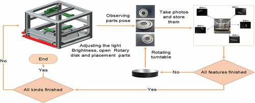
This paper designs and builds a multi-channel data acquisition system, which is shown in Figure 1. The acquisition system includes an image acquisition module, data storage module, part position conversion module, and data processing module. The image acquisition module is principally composed of a set of cameras and a concurrent calling mechanism pro-gram. Multiple cameras simultaneously collect data. Images are captured in the same space to shoot time-consistent parts data, called space-time consistency parts data. The data storage module is used to receive the collected image and permanently preserve the picture. The function of the part position conversion module is to reduce manual operation and change the part poses. The data processing module stores the data in batches to remove noise, clipping, and data enhancement operations.

The acquisition process calls the image acquisition module and concurrently collects the data from multiple cameras. After a set of data acquisitions, the data is transmitted directly to the storage module for persistent storage. Then, the part’s pose is changed by the rotation base driver, and the data images with different poses of the same part are obtained and repeatedly saved. Finally, the image stored in persistence is denoised, binarized, edge determined and stored in the specified position.

Data Preprocessing

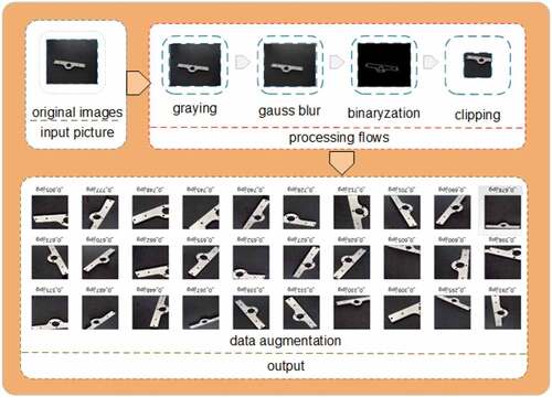
The photos collected in this paper are 640 * 480 pixels. The background of the parts images is a single black background that does not contain any com-plex information. The deep neural network can eliminate background interference background. To re-duce the computational complexity and remove use-less information, the data set cuts the parts along the edge and scales them to 80 * 80 pixels, which retains the most critical shape features of the parts.

Through the experiment, it is found that the acquisition requirements for the external environment are more stringent. Due to the fact that the external light environment exerts considerable interference on part image acquisition, a weak white lateral light source in a closed space is designed to effectively avoid reflection of the parts under the lens. At the same time, the part images are taken under the condition of darkfield illumination since insufficient illumination will produce Gaussian noise in the lens. The white noise causes errors during edge detection of the part when the part image is binarized, resulting in errors in data cutting. Therefore, Gaussian blur is used to process the image noise to realize filtering noise in binarization. During the following process, the key to cutting the part’s data boundary is to determine the part’s boundary information. The canny operator is used for edge detection to obtain the edge length in the long and wide directions. The maximum value of the two is calculated as the edge length of the intercepted square, and then the image is zoomed to 80 * 80 pixels.

Deep learning requires considerable image data. The shooting methods used to acquire that data consume many human resources and material resources. Therefore, the data enhancement method is adopted. First, the range of the rotation angle, the proportion of the offset, and the proportion of the zoom of the image are set in advance, and then the new image is generated by random batch processing. After integrating the generated image and the original data, the image of each part is divided into the uncoupling disjoint training set, verification set and test set. The part data after data enhancement is shown in Figure 2.

Figure 2. Data set processing flow.

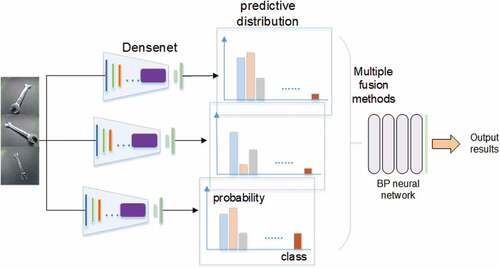
Method

It is challenging to use a single model to fit all the data, and the accuracy is poor when identifying simi-lar parts. Therefore, the two-stage model is used to make predictions. In the first stage, the DenseNet structure is used to predict the single side image. In the second stage, the BP neural network is used to predict three sides.

DenseNet Structure

For industry, small models can significantly save bandwidth and reduce storage overhead. The num-ber of parameters required for DenseNet is less than half of ResNet. And to achieve the same accuracy as ResNet, DenseNet requires only about half of Res-Net’s computation. DenseNet has very good anti-overfitting performance, especially suitable for applications where training data are relatively scarce. In this paper, the de novo training densenet is used as the image data feature extraction deep learning model. Unlike ResNet, DenseNet does not use the transmission of residuals, nor does it use the idea of inception to increase the network width; it instead proposes another improvement method. DenseNet achieves a nonlinear change in each layer, where i represents the i layer, the output of the i layer is denoted as $x_i$, and its connection mode is a direct connection from any layer to the back layer. Then, the feature input of all layers in the front of the i layer is obtained, $x_0$ and $x_1$, $x_{n-1}$. such as in the formula:

(1) $x_i=H_i([x_0,x_1,\dots ,x_{i-1}])$(1)

The operation $H_i(.)$ is defined as three continuous functions: BN, ReLU, and Conv3*3.

To solve the problem that the feature map cannot be cascaded after convolution, DenseNet divides the network structure into several closely connected block networks, called dense blocks. This model has a fast convergence speed and high classification ac-curacy and recognition rate. Therefore, to achieve the best effect, the DenseNet network is selected as the model for single feature extraction.

Design of Multi-side W Detection Model

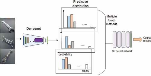
Several surfaces of the various parts mentioned above may have the same shape and color as other parts, and that similarity confuses the deep learning process. In these situations, the part type cannot be distinguished, which results in a decline in prediction accuracy. This paper proposes two model prediction methods: a single-channel multi-input model and multi-channel multi-input model. The idea of ensemble learning multi-model fusion is used for reference. Both models use multiple pictures that are input together. After inputting the images to the model, their prediction results are input into the backpropagation neural network as features for the next round of learning. At the same time, three feature fusion methods are proposed for feature combination, and experiments are conducted.

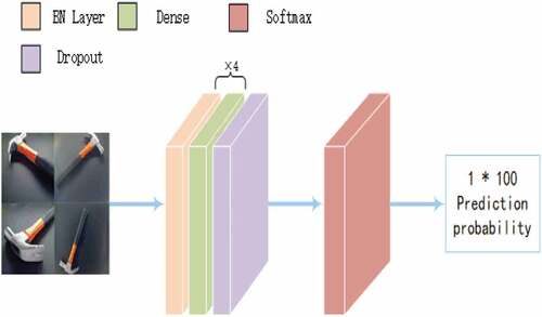
BP Neural Network Structure

Considering that there are 100 part types in this experiment as well as the size of the fusion feature matrix and the final number of classified parts after the three images are input, it was decided that the neural network should be designed as a shallow net-work; a shallow network can meet the requirements of accurate classification and accelerate the model training. The BP neural network for classification of 100 types of parts comprises 13 layers of three net-work structures, namely a Dense layer, Dropout layer, and BatchNormalization layer. The activation function of the Dense layer is ReLU, and the number of neurons is set to 100 per layer. The parameter setting for the Dropout layer is 0.4 to reduce the overfitting phenomenon; 40% of the parameters are randomly selected as 0 during the training process. The BatchNormalization layer is used to normalize each batch of data to prevent gradient dispersion and further improve the learning efficiency. The BP neural network’s structure is shown in Figure 3.

Figure 3. Design of second layer neural network.

Space-time Consistency Image Feature Fusion Method

The method proposed in this paper is the multi-input joint detection method. The first layer model inputs three images of the same part that are consistent in time and space and are at different angles. Then, the model outputs the probability matrix of the prediction for these three images. The method for combining multiple sets of features is critical. The feature combination method directly affects the prediction effect of the second layer model. This paper proposes three methods for combining multi-input prediction results. It is assumed that the prediction results for the first image are $A=[a_1,a_2,\dots \dots ,a_n{]}_{\hspace{0.17em}}$ and that the prediction results for the second and third images are $B=[b_1,b_2,\dots \dots ,b_n]$ and $C=[c_1,c_2,\dots \dots ,c_n]$, respectively. The digital in each matrix predicts this image’s content as the probability of each part, and the digital subscript represents the part’s label.

The first feature fusion method expands the dimension of the feature probability matrix. The dimension of the augmented matrix fuses multiple matrices to extend the matrix by increasing the dimensions. The matrix expansion forms different features at different latitudes, creating various input feature matrices. The first fusion method expands the 0th dimension of the matrix. It concatenates the first matrix with the second matrix. Two matrices with dimensions of 1 * 100 are combined to obtain a matrix with dimensions of 1 * 200. Similarly, the obtained 1 * 200 matrix is combined with 1 * 100 to obtain a matrix with a final feature input of 1 * 300. To construct the fused feature input $D_1$:

(2) $D_1=concatenate(A,B,C)$(2)

The results of $D_1$ are:

$[a_1,a_2,\dots ,a_n,b_1,b_2,\dots ,b_n,c_1,c_2,\dots ,c_n]$

.

The second feature fusion method is feature addition, which ensures that the dimension before feature fusion is consistent with the dimension after feature fusion. The three feature matrices are 1 * 100. This fusion method adds the prediction probability of the corresponding dimension to obtain the exact size of the 1 * 100 prediction probability matrix. It does not distinguish the order and relative position of the three prediction matrices. If the feature input after fusion is $D_2$, then $D_2$ is expressed by the formula:

(3) $D_2=A+B+C$(3)

The results of $D_2$ are:

$[a_1+b_1+c_1,a_2+b_2+c_2,\dots ,a_n+b_n+c_n]$

.

The third fusion method combines the first and second fusion methods. It considers the situation in which three types of prediction probability matrices expand in the same dimension. At the same time, the three types of prediction probability matrices are added by the same latitude expansion method. After the second feature reorganization, the feature matrix is added to the back of the first method at the same latitude. Let the fused feature input be $D_3$. Then, $D_3$ is expressed by the formula:

(4) $D_3=concatenate(D_1,D_2)$(4)

The results of $D_3$ are:

$[a_1,a_2,\dots ,a_n,\dots c_1,c_2,\dots ,c_n,a_1+b_1+c_1,\dots a_n+b_n+c_n]$

.

Multi-channel Multi-input Model

After the parts are placed on the turntable, they are photographed from three different angles to obtain the characteristics of different positions simultaneously; these characteristics are directly divided into three groups of data sets that do not intersect but belong to the same category. The multi-model prediction method is used to maximize the recognition accuracy and obtain the best effect in the actual industrial production situation. The three independent basic models are trained, and three images are collected and input into the three models trained by the corresponding angle data to obtain the prediction result matrix. Then, the predicted result matrix is treated with the three fusion methods mentioned above and sent to the BP neural network in the second part for two-stage identification. The prediction result for the final part type number is the subscript of the maximum number in the BP neural network’s prediction matrix. The multi-channel multi-input model structure is shown in Figure 4.

Figure 4. Multi-channel multi-input model.

Single-channel Multi-input Model

The first phase of a single-channel model predicts that only one DenseNet network structure is used to mix the three data sets into a group for training the multi-channel model, and the same test set is mixed into a group. The training set and test set contain three times the amount of data for each multi-channel model. The three angle images are preprocessed and input into DenseNet to obtain the prediction matrix for the three images. Then, the features are combined using various fusion methods, and the processed features are transmitted to the BP neural network as the first model. The final prediction for the part number is also the subscript of the maxi-mum number in the matrix generated by the BP net-work. The structure of the single-channel multi-input model is shown in Figure 5.

Figure 5. Single-channel multi-input model.

Experimental Results

The experimental platform is a GTX1080ti, we built the Densenet network in the open-source keras artificial neural network library using VS Code, and there are a total of 100 part categories. The original collection data consists of three groups of data, each with 6,000 samples, for a total of 18,000 samples. Among them, there are 180 pictures for each type of part (60 pictures for each angle), and the number of samples after data enhancement is 150,000, and then the training set, validation set, and test set are divided according to the ratio of 25:1:1. The three groups of data cameras numbered in this experiment are 1, 2, and 3. Since the polyhedron has six opposite sides, it is necessary to input all six sides into the model to accurately identify them in the worst case, and there is a plane at the bottom that contains the parts. Therefore, side data of up to five angles are collected. When the direction of the collected image is greater than or equal to three, it is necessary to rotate the parts at least twice to shoot all six sides. The same model also needs to run at least twice for identification. When the acquisition direction is two, the model needs to run three times for identification. When the acquisition direction is one, it needs more model runs. Therefore, considering the above factors, the actual production demand, and efficiency, the final number of joint identification sides is three. After taking out the three groups of data, each group is used to train a model. At this time, three different deep learning models obtained from training three data groups are obtained. At this point, the accuracy of the three models is shown in Table 1. Model 1 represents the shooting data training model from camera one.

Table 1. Comparison of the highest training accuracy for 100 different parts models.

Category	Model 1	Model 2	Model 3	Traditional Model
Accuracy	80.500%	87.000%	88.000%	88.500%

In the general training of a deep learning model, the training principle inputs all the data taken from all angles into the model for training and then inputs an image into the model when the model is used. Therefore, this paper uses the traditional training method as a control and mixes each training set and a test set from the three data groups into a control group. When the data set contains 100 part types, the results are as follows in Table 1 and Figure 6 (a):

Figure 6. Model accuracy on test set. (a) accuracy of multiple models. (b) accuracy information of the test set for the multi-channel model during different training rounds. (c) test set accuracy for the single-channel model during different training rounds.

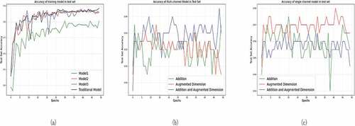
It can be seen from the results of the comparative experiment that the accuracy of the part data set from the three groups of mixed-data training models on the test set is almost equal to that of each group’s data training model. This result occurs because the third part of the previous analysis has multiple feature surfaces, one of which is used for classification. Different classes are most likely to use shape-like feature surfaces for training and cannot learn the different points of different categories, so some of the contents learned during this exercise are incorrect.

The following experiments show the final prediction results for the two different models using different methods combined with the characteristics after the first stage of prediction. The data sets containing 100 parts are used for the experiments, and two pieces from each class are used as test sets to calculate the final prediction accuracy. In this experiment, BP neural network of the second layer uses the Densenet layer, the BatchNormalization layer and the Dropout layer of the Keras artificial neural network library. The network sets the learning rate = 0.001, the deactivation ratio is 0.4, and uses 50 epochs for training, and the FPS of the network reaches 144FPS. The selected optimizer is Adam. The selected loss function is a cross-entropy loss function.

(5) $loss=-\sum _{i=1}^n{\hat{y}}_{i1}log{y}_{i1}+{\hat{y}}_{i2}log{y}_{i2}+\dots +{\hat{y}}_{im}log{y}_{im}$(5)

where n is the sample number and m is the classification number.

The accuracy changes in the different multi-channel and multi-model feature fusion methods on the test set are shown in Figure 6 (b). The average accuracy of the test set obtained by the addition fusion method and the dimension expansion fusion method are roughly similar. The accuracy of the test set obtained by the dimension expansion fusion method is higher than the other two, and the highest accuracy is 94.5%, which is and higher than the traditional training method: the three-channel data fusion model training strategy improved the accuracy by 6%. This method can apply to the actual production environment.

Figure 6 (c) shows the accuracy changes of different feature fusion methods using single-channel multi-input on the test set. In this model framework, all feature fusion methods have higher average accuracy than the multi-channel multi-input model, and the average accuracy of each fusion method is improved by 2% – 3%. The results obtained by adding fusion features are roughly the same as those obtained by adding dimension expansion. The accuracy of the test set obtained by feature fusion using dimension expansion is still up to 98%, and it can be fully applied to the actual production environment to obtain more accurate prediction results.

The two models use different feature fusion methods to obtain the highest accuracy on the test set, as shown in Table 2.

Table 2. Test set accuracy of two models with different fusion methods.

Model category	Additive fusion	Augmented fusion	Additive dimension expansion fusion
Multi-channel multi-input model	93.500%	94.500%	93.500%
Single-channel multi-input model	97.500%	98.000%	96.500%

After comparison, it is found that the accuracy of the fusion model proposed in this paper is approximately 10% higher than that of the single model trained by the mixed data set for the three shooting angles and the model trained using a lens angle data set. The effect of the single-channel multi-input model is better than that of the multi-channel multi-input model. The accuracy of the feature fusion that uses the single-channel multi-input to expand the dimension of the feature is higher than that of the other five methods.

Conclusion

Against the background of intelligent manufacturing, the scale and quantity of production are increasing each day. Intelligent warehousing effectively solves problems that arise from the industrial production process and inventory. The rapid identification of many industrial material parts is the key to effectively improving the efficiency of the industrial pro-duction process and intelligent warehousing. Accu-rate identification of both similar and special parts is an important problem. Nonstandard parts cannot be identified using two-dimensional codes; image feature identification is therefore needed. This paper designs a multi-channel visual acquisition system for constructing a space-time consistency industrial part data set. The joint identification method for multi-side acquisition is proposed to solve the classification problem for similar parts. When using the fusion model for classification, compared to the original DenseNet method, the multi-channel multi-input model prediction achieves an accuracy improvement of approximately 6%, and single-channel multi-input model prediction achieves an accuracy improvement of approximately 10%. The method proposed in this paper provides a new strategy for the identification of industrial parts. A method for effectively identifying damaged and rusted parts after use is the focus of future industrial part identification research.

Disclosure Statement

No potential conflict of interest was reported by the author(s)

Additional information

Funding

This work was supported by the National Natural Science Foundation of China (Fund No. 1) (Grant No. 62073245), the Natural Science Foundation of Shanghai (20ZR1440500), Science and Technology Research Program of Chongqing Municipal Education Commission (Grant No. KJQN201901133), National Natural Science Foundation of China (Fund No.2) (Grant No. 51806145).

References

- Cao, L., and X. Wei. 2020. Application of Convolutional Neural Network Based on Transfer Learning for Garbage Classification.2020 IEEE 5th Information Technology and Mechatronics Engineering Conference (ITOEC). IEEE, Chongqing, China: 1032–2666. doi:10.1109/ITOEC49072.2020.9141699.
- Chung, F. J. K., C. Y. Shih, and J. Y. Lee. 2008. Separating color and identifying repeat pattern through the automatic computerized analysis system for printed fabrics. Journal of Information Science and Engineering 24 (2):453–67.
- Demizio, D. J., and E. J. Bernstein. 2019. Detection and classification of systemic sclerosis-related interstitial lung disease: A review. Current Opinion in Rheumatology 31. doi:10.1097/BOR.0000000000000660.
- Elsisi, M., T. Minh-Quang, M. Karar, L. Matti, and M. M. F. Darwish. 2021. Deep Learning-Based Industry 4.0 and Internet of Things towards Effective Energy Management for Smart Buildings. Sensors 21 (4):1038. doi:10.3390/s21041038.
- Fu, P., J. Wang, X. Zhang, L. Zhang, and R. X. Gao. 2020. Dynamic routing-based multimodal neural network for multi-sensory fault diagnosis of induction motor. Journal of Manufacturing Systems 55 (4):264–72. doi:10.1016/j.jmsy.2020.04.009.
- Huang, G., Z. Liu, and V. Laurens. 2017. Densely Connected Convolutional Networks. Computer Vision and Pattern Recognition (CVPR) 2261–69. doi:10.1109/CVPR.2017.243.
- Ioffe, S., and C. Szegedy. 2015. Batch Normalization: Accelerating Deep Network Training by Reducing Internal Covariate Shift. International conference on machine learning,PMLR, Lille, France, Volume 37 ( ICML’15): JMLR.org, 448–56.
- Kaiming, H., Z. Xiangyu, R. Shaoqing, and S. Jian. 2016. Deep Residual Learning for Image Recognition. Proceedings of the IEEE Conference on Computer Vision and Pattern Recognition (CVPR), LAS VEGAS pp. 770–78. doi: 10.1109/CVPR.2016.90
- Krizhevsky, A., I. Sutskever, and G. Hinton. 2012. Imagenet classification with deep convolutional neural networks. Advances in Neural Information Processing Systems. 1097-1105, 84–90. doi:10.1145/3065386.
- LeCun, Y., Y. Bengio, and G. Hinton. 2015. Deep learning. Nature 521 (7553):436. doi:10.1038/nature14539.
- LeCun, Y., L. Bottou, Y. Bengio, and P. Haffner. 1998. Gradientbased learning applied to document recognition. Proceedings of the IEEE 86 (11):2278–324. doi:10.1109/5.726791.
- Li, P., Z. Tan, L. Yan, and K. Deng. 2011. Time series prediction of mining subsidence based on a SVM. Mining Science and Technology Pages:557–62. doi:10.1016/j.mstc.2011.02.025.
- Li, X., W. Zhang, and X. Bian. 2004. Research on lane marking detection based on machine vision. Journal of Southeast University 20 (2):176–80. doi:10.1007/978-3-642-25185-6_69.
- Meriama, M., and B. Mohamed. 2018. Automatic adaptation of SIFT for robust facial recognition in uncontrolled lighting conditions. IET Computer Vision 12 (5):623–33. doi:10.1049/iet-cvi.2017.0190.
- Roy, S., M. Willi, O. Sebastiaan, L. Ben, F. Enrico, S. Cristiano, H. Iris, C. Nishith, M. Federico, S. Alessandro, et al. 2020. Deep Learning for Classification and Localization of COVID-19 Markers in Point-of-Care Lung Ultrasound. IEEE Transactions on Medical Imaging. doi: 10.1109/TMI.2020.2994459.
- Russakovsky, O., J. Deng, H. Su, J. Krause, S. Satheesh, S. Ma, Z. Huang, A. Karpathy, A. Khosla, M. Bernstein, et al. 2015. ImageNet Large Scale Visual Recognition Challenge. International Journal of Computer Vision 115 (3):211–52. doi:10.1007/s11263-015-0816-y.
- Sener, B., G. Ugur, O. Murat, and U. Hakki Ozgur. 2021. A novel chatter detection method for milling using deep convolution neural networks. Measurement 182:109689. doi:10.1016/j.measurement.2021.109689.
- Shah, M., L. Ana, and R. Jens. 2020. Automated classification of normal and Stargardt disease optical coherence tomography images using deep learning. Acta Ophthalmologica 98 (6). doi: 10.1111/aos.14353.
- Szegedy, C., S. Ioffe, V. Vanhoucke, and A. Alemi. 2017. Inception-v4, Inception-ResNet and the Impact of Residual Connections on Learning. Thirty-first AAAI conference on artificial intelligence, San Francisco, California USA.
- Szegedy, C., W. Liu, Y. Jia, P. Sermanet, and A. Rabinovich. 2015. Going Deeper with Convolutions. Computer Vision and Pattern Recognition (CVPR) 1–9. doi:10.1109/CVPR.2015.7298594.
- Szegedy, C., V. Vanhoucke, S. Ioffe, J. Shlens, and Z. Wojna. 2016. Rethinking the Inception Architecture for Computer Vision. IEEE Conference on Computer Vision and Pattern Recognition (CVPR), LAS VEGAS, IEEE:2818–26. doi: 10.1109/CVPR.2016.308
- Xiaojun, B., and W. Haibo. 2019. Early Alzheimer’s disease diagnosis based on EEG spectral images using deep learning. Neural Networks. Neural Networks 114. doi:10.1016/j.neunet.2019.02.005.
- Xie, Y., T. Niu, S. Shao, Y. Zhao, and Y. Cheng. 2020. Attention-based Convolutional Neural Networks for Diesel Fuel System Fault Diagnosis.2020 International Conference on Sensing, Measurement & Data Analytics in the era of Artificial Intelligence (ICSMD), Xi'an, China. 210–14. doi: 10.1109/ICSMD50554.2020.9261700.