Optimizing Berth-quay Crane Allocation considering Economic Factors Using Chaotic Quantum SSA

ABSTRACT

With the regular development of the global epidemic, the global port shipping supply is tight. The problem of port congestion, soaring freight rates, and hard-to-find container space has emerged. This paper proposes a new joint berth-quay crane allocation model, namely E-B&QC, by taking the minimum of the time in the port of the ship, the cost of extra transportation distance for collector trucks in the land area of the port, and the cost of extra waiting time for ships. Then, the deficiencies of the sparrow search algorithm (SSA) are considered in solving the E-B&QC model, and the SSA is improved based on the three-dimensional Cat chaos mapping and quantum computing theory. Chaotic Quantum Sparrow Search Algorithm (CQSSA) is proposed, population individual coding rules are formulated, also E-B&QC model solving algorithm is established. Finally, a new berth-crane allocation optimization method, namely, E-B&QC-CQSSA, is proposed. Subsequently, the feasibility and superiority of the proposed allocation model and solution algorithm are tested according to the actual data of a small river port in the south and a medium-sized river port in the north. Simulation examples show that the E-B&QC model can develop different high-quality solutions for container ports under different working conditions, and the more complex the actual situation of the port, the more significant the optimization effect. The proposed CQSSA for E-B&QC model can obtain a better solution.

KEYWORDS:

• Berth quay crane joint distribution
• Optimization model
• Economic benefits
• Sparrow Algorithm
• Quantum theory
• Chaos theory

Introduction

With the development of the economy, the requirements for container port logistics and transportation have been increased gradually. As the container port handling operations are more linked, the process is more complex, the container port needs to be integrated research. How to reduce the cost of container ports and improve the efficiency of container port collection and distribution has become the focus of research. The distance between the ship berth and the container yard affects the distance of container truck transportation. The reasonable allocation of berths can not only reduce the waiting time of ships but also reduce the cost of port operations. In addition, the reasonable allocation of the quay crane can improve the efficiency of ship loading and unloading operations, while reducing the time of loading and unloading operations. Therefore, joint berth-quay crane scheduling can improve the efficiency of container port handling operations, reduce the total operating costs of container ports, and improve the satisfaction of customers and port managers (Liu, Wang, and Shahbazzade 2019). Delayed vessel departures can also result in additional vessel waiting times for vessels and container ports. The cost of additional vessel waiting time is reduced, which can achieve the purpose of reducing vessel time in port and improving the efficiency of container port handling operations (Yang et al. 2016).

In this paper, research work is carried out on the hot issues of container port dispatch and allocation schemes. This paper especially considers the impact of economic factors on container ports, analyzes the balance between economic benefits and operational efficiency and aims to reduce the time of ships in port, the cost of truck transportation, and the cost of port services, to obtain a higher quality container port berth-quay crane joint dispatch plan.

The rest of this paper is organized as follows: Section 2 introduces the research status of research models and algorithms; Section 3 introduces the E-B&QC model established in this paper; Section 4 describes the proposed algorithm of the CQSSA applicable to the E-B&QC model and provides the solution method for the berth-crane allocation optimization model; Section 5 presents the data test simulation study of this model and analyzes the performance of the proposed model as well as the algorithm in this paper; Section 6 draws conclusions.

Literature Review

Berth-quay Crane Joint Dispatch and Assignment Problem (B&QAC)

In recent years, scholars have conducted research on the berth-quay crane allocation problem. A list of literature for B&QAC can be viewed in Table 1. Karam and Eltawil (2016) proposed a new optimization model for the berth-quay crane scheduling optimization problem, which was verified to be feasible and superior through numerical calculations and theoretical analysis. For the problem of unreasonable resource scheduling of container terminals, Yang et al. (2016) established a berth-quay crane optimization model with minimizing the total vessel service cost as the objective function according to the actual situation of terminals. Li et al. (2017) proposed a multi-objective discrete berth-quay crane allocation model to improve the effectiveness and optimization efficiency of berth-quay crane allocation in container ports with the optimization objectives of minimizing the container truck distance and vessel time in port. And the chaotic cloud particle swarm algorithm is used to solve the berth-quay crane assignment model, a particle feasible-integration processing module is developed and embedded in the evolution of the chaotic cloud particle swarm algorithm, the particle coding rules are formulated, the calculation methods of particle history extrema and global extrema of multi-objective functions are designed, and a new method based on the chaotic cloud particle swarm optimization algorithm is proposed to solve the multi-objective discrete berth-quay crane assignment model, and the numerical calculation results prove the feasibility and practicality of the proposed model and algorithm. Thanos et al. (2021) created a new mathematical model for the allocation problem of continuous berths in container ports with a specific quay lift operation problem, and based on this, proposed a mathematical formulation to solve this problem using a heuristic algorithm, and analyzed it in comparison with traditional methods in the context of the actual situation of container ports. For the problem of joint berth-quay crane allocation and optimal scheduling, based on rolling heuristic algorithm, Rodrigues and Agra (2021) provided a quality solution for the joint berth-quay crane allocation problem. Vrakas, Chan, and Thai (2021) enhanced the RBV theory for improving the performance of container port operations and made a study based on the Patrick Terminal example in Australia to provide a more effective solution for container port management. For the integrated scheduling problem of automated container terminal berths and quay cranes under uncertainty, Wu and Zhu (2021) proposed a decision framework combining active and responsive scheduling strategies, constructed a recovery objective cost minimization mixed-integer programming model, and proposed an improved adaptive genetic algorithm for solving the model. Cho, Park, and Lee (2020) proposed a new heuristic greedy stochastic adaptive search method for the joint container port berth and quay crane allocation problem, which was verified its feasibility and superiority by an actual container terminal in Busan, Korea.

Table 1. List of literature for B&QAC

Literature	Contribution
Karam and Eltawil (2016)	A new berth-quay crane joint optimal scheduling scheme to provide a solution for the joint allocation of berth-quay cranes is proposed
Yang et al. (2016)	An optimal scheduling scheme to minimize the total cost of ship service is proposed
Li et al. (2017)	An optimal scheduling scheme based on the chaotic quantum particle swarm algorithm to minimize the truck distance and the ship’s time in port is proposed
Thanos et al. (2021)	A new berth-quay crane joint dispatch scheme based on continuous berth is proposed
Rodrigues and Agra (2021)	A berth-quay crane joint scheduling scheme based on a rolling heuristic algorithm is proposed
Vrakas, Chan, and Thai (2021)	A port scheduling scheme aiming at improving container port performance is proposed
Wu and Zhu (2021)	An optimization model of berth-quay crane dispatching under uncertain factors is proposed
Cho, Park, and Lee (2020)	A berth-quay crane scheduling optimization model based on a new heuristic greedy random adaptive search method is proposed

In the above research, the operation time of container port ships and the truck transportation route are optimized to improve the utilization efficiency of container port berths and quay cranes. Based on this research, this paper considers the influence of ship’s time in port and truck transportation distance on the allocation of quay cranes in container ports and additionally considers economic factors to construct an optimization model to obtain a better berth quay crane allocation program.

Based on the above problems, this paper conducts research on the construction of a new berth-quay crane joint dispatch allocation model. In this paper, the berth-quay crane allocation optimization problem is considered from the perspective of economic efficiency of container ports, considering the time of the ship in port, the cost of extra transportation distance for collector trucks in the land area of the port, and the cost of extra waiting time for ships. In addition, this paper sets preference weighting coefficients to satisfy the different needs of container ports under different working conditions. Thus, a new berth-quay crane optimization model (E-B&QC) accounting for economic factors is constructed in this paper, by taking the minimum of the time in the port of the ship, the cost of extra transportation distance for collector trucks in the land area of the port, and the cost of extra waiting time for ships as the optimization objectives.

The Sparrow Search Algorithm (SSA)

The research shows that the accuracy of solving the joint berth-quay crane scheduling model determines whether a better-quality solution can be obtained for the container terminal. In order to solve the joint berth-shore-bridge scheduling model, a wide range of scholars have used different methods to solve it. The Sparrow Search Algorithm (SSA) (Xue J, Shen, and Xue 2020) is a novel group optimization method inspired by the intelligence, foraging, and anti-predatory behavior of sparrow groups. After the comparison test of 19 basic functions and traditional intelligent optimization algorithms (Xue J, Shen, and Xue 2020), the SSA has a more excellent performance in terms of accuracy, convergence speed, stability, and robustness, so this paper tries to use the SSA to solve the E-B&QC model. However, like traditional swarm intelligence optimization algorithms, the evolutionary late-stage SSA suffers from the shortcomings of easily falling into local optimum, poor global searchability, and slow convergence. In response to the shortcomings of SSA, scholars have conducted research on its improvement. A list of literature for SSA can be viewed in Table 2. Song W et al. (2020) used chaotic methods with tilted tent maps to generate initialized populations to improve population quality, introduced nonlinear decreasing weights to improve location updates and increase search efficiency, moreover, they introduced variation strategies and chaotic search to increase population diversity. Liu and Wang (2021) introduced Circle chaotic map in generating populations to improve its global search ability at the beginning of iterations. At the same time, T-distribution variation was introduced to affect the update rule of sparrow population location for different iteration cycles. Finally, a “similarity function” is constructed to measure the “dispersion” of the sparrow population, and a search rule for the sparrow population under different “dispersion” is developed. Yang et al. (2021) combined the particle swarm algorithm and the SSA so that the SSA individuals converge faster before updating and constructing the fitness function based on the maximum likelihood estimation of the parameters for the initialization of the parameters. Yuan et al. (2021) used the center of gravity reverse learning mechanism to initialize the population position update, introduced learning coefficients in the position update part of the discoverer to increase its global search ability, and also used variational operators to improve the positions of other populations to avoid them from falling into local optimum. Liu et al. (2021) introduced a chaos strategy in the SSA to enhance the diversity of the algorithm population and used adaptive inertia weights to balance the convergence speed and exploration ability of the algorithm. Finally, the Cauchy-Gaussian variation strategy is used to enhance the ability of the algorithm to get rid of stagnation. Wang, Zhang, and Yang (2021) dealt with the problem that the population diversity of the basic sparrow search algorithm will be gradually lost in the later stages of evolution, which reduces and easily falls into local extremes in the later iterations of the basic sparrow search algorithm, proposed a chaotic sparrow search algorithm based on Bernoulli chaos mapping, Dynamic Adaptive Weighting, Cauchy Mutation, and inverse learning, which was tested and waited for a better convergence speed as well as computational accuracy. OuOuyang, Zhu, and Qiu (2021) proposed a lens learning sparrow search algorithm (LLSSA), the algorithm introduces a backward learning strategy based on the lens principle to improve the search range of individual sparrows, and then proposes a variable spiral search strategy to make the followers’ search more detailed and flexible, and finally combines the simulated annealing algorithm to judge and obtain the optimal solution.

Table 2. List of literature for SSA

Literature	Contribution
Song W et al. (2020)	Chaotic methods are used with tilted tent maps to improve SSA
Liu and Wang (2021)	Circle chaotic map and T-distribution variation to improve SSA is introduced
Yang et al. (2021)	Particle Swarm Optimization with SSA is combined
Yuan et al. (2021)	A barycentric inverse learning mechanism is used to update initialized population location and variational operators are used to refining the population location
Liu et al. (2021)	Chaos Mechanisms, Adaptive Inertial Weights, and Cauchy-Gaussian Variation Strategies are used to improve SSA
Wang, Zhang, and Yang (2021)	An SSA based on Bernoulli chaotic map, dynamic adaptive weighting, Cauchy mutation, and reverse learning is proposed
OuOuyang, Zhu, and Qiu (2021)	A shot learning sparrow search algorithm (LLSSA) is proposed

The existing research on the SSA has improved the optimization performance of the algorithm, but there is still much room for improving the global search ability and jumping out of the local optimal solution of SSA. In this paper, to improve the global search capability of the SSA to avoid falling into local optimal solutions at the late stage of the algorithm, to increase the global perturbation capability, and to ensure the accuracy and timeliness of solving the E-B&QC model, this paper improves the SSA and proposes a chaotic quantum sparrow search algorithm based on quantum computing and 3D chaotic mapping. The algorithm uses the principle of quantum computing to improve the position update formula of the discoverer part of the sparrow population to efficiently enhance the global search capability; it introduces a three-dimensional Cat mapping to perturb the population individuals that fall into the local optimum at the late evolutionary stage to increase the population diversity at the late evolutionary stage of the algorithm. Finally, the optimization method of berth quay crane scheduling based on the CQSSA solving the E-B&QC model, namely, E-B&QC-CQSSA, is established. In order to test the feasibility of the proposed model and algorithm, simulation experiments are carried out based on the actual operational data of the port.

Establishment of E-B&QC Model

This paper focuses on constructing the E-B&QC optimization model from the perspective of the total cost of the container port area. In the process of container port berth-quay crane scheduling optimization, the continuous container port shoreline is divided into several independent berths, i.e. discrete berths. In the process of vessel docking, according to the actual situation, the vessel is required to be allowed to dock only once and is not allowed to dock across the berths. In the process of the model, the ship is limited to performing a complete loading and unloading operation process only once. In addition, it is required that during the loading and unloading operation of the quay crane, only one ship is allowed to carry out loading and unloading operations at the same time. The berthing sequence of ships, the allocation of berths, and the allocation of cranes should minimize the time of ships in port, the cost of extra transport distance for trucks in the land area of the port, and the cost of extra waiting time for ships.

Assumptions and Notations

When constructing the E-B&QC model, the following 10 assumptions are constructed from the berth and quay crane perspectives, respectively, according to the berth-quay crane allocation optimization process:

1. Ship arrival time is known;

2. Each ship has a predetermined berth, and when the ship is moored at the predetermined berth, the distance of transportation of the collector truck is the shortest;

3. Vessel berthing positions all satisfy the requirements of physical conditions such as water depth and ship length;

4. Each ship has one and only one berthing opportunity;

5. The number of quay cranes for loading and unloading service of the ship remains the same during the loading and unloading process of the ship;

6. Ship loading and unloading operations to meet the requirements of the maximum and minimum number of allocable quay cranes;

7. The time of the quay crane movement during the loading and unloading operation is not considered;

8. Quay crane operations are not allowed to move across other quay cranes;

9. The quay crane cannot be stopped in the middle of the operation until the end of the loading and unloading task;

10. All quay crane work efficiency is the same. The impact of quay crane maintenance, the rest of the workers, and other factors on the time are not considered.

The notation of the E-B&QC model used in this paper is summarized in the following:

VArriving Ship (V= {1, 2, …, v})

B Berth (B= {1, 2, …, b})

CCrane (C= {1, 2, …, c})

αUnit time cost of waiting for a vessel to berth after arrival

γUnit time cost of delayed vessel departure;

VOShip berthing sequence set;

VBShip berth set;

VCNumber of quay cranes for ship operations;

VO_iShip i berthing sequence;

VB_iShip i berth;

VC_iNumber of quay cranes allocated by ship i plan;

TA_iArrival time of ship i;

TB_iShip i berthing time;

TS_iShip i start loading and unloading operation time

TF_iThe departure time of ship i;

TD_iThe distance between the actual berth of the ship i and the preferred berth;

TQ_iThe estimated departure time of ship i;

VP_iThe preferred berth of the ship i

VE_iLoading and unloading container volume of the ship i;

CE₀Single quay crane loading and unloading efficiency;

VCm_iThe minimum number of quay cranes acceptable to ship i

VCM_iThe maximum number of quay cranes acceptable to ship i;

VL_iSafety captain of the ship i (including lateral safety reserve distance)

VD_iSafety water depth of ship i (including longitudinal safety reserve distance);

BL_jLength of berth j;

BD_jFront water depth of berth j;

x_ijk and q_in are defined variables, determined in the following way:

$x_{ijk}=\left\{\begin{array}{c}1\mathrm{i}\mathrm{f}\mathrm{s}\mathrm{h}\mathrm{i}\mathrm{p}i\mathrm{s}\mathrm{e}\mathrm{r}\mathrm{v}\mathrm{e}\mathrm{d}\mathrm{a}\mathrm{c}\mathrm{c}\mathrm{o}\mathrm{r}\mathrm{d}\mathrm{i}\mathrm{n}\mathrm{g}\mathrm{t}\mathrm{o}\mathrm{s}\mathrm{e}\mathrm{q}\mathrm{u}\mathrm{e}\mathrm{n}\mathrm{c}\mathrm{e}k\mathrm{a}\mathrm{t}\mathrm{b}\mathrm{e}\mathrm{r}\mathrm{t}\mathrm{h}j\\ 0\mathrm{e}\mathrm{l}\mathrm{s}\mathrm{e}\end{array}\right.$

$q_{in}=\left\{\begin{array}{c}1\mathrm{i}\mathrm{f}\mathrm{q}\mathrm{u}\mathrm{a}\mathrm{y}\mathrm{c}\mathrm{r}\mathrm{a}\mathrm{n}\mathrm{e}n\mathrm{s}\mathrm{e}\mathrm{r}\mathrm{v}\mathrm{e}\mathrm{s}\mathrm{f}\mathrm{o}\mathrm{r}\mathrm{s}\mathrm{h}\mathrm{i}\mathrm{p}i\\ 0\mathrm{e}\mathrm{l}\mathrm{s}\mathrm{e}\end{array}\right.$

Among the above-mentioned variables, VO, VB, VC, VOi, VBi, and VCit are the decision variables of the E-B&QC model, while TBi, TSi, TEi, xijk, and qitn, are the dependent variables of the E-B&QC model.

Determination of Objective Function F

To minimize the total cost of container port area and improve the economic efficiency of the container port, this paper constructs the E-B&QC optimization model, by taking the minimum of the time in the port of the ship, the cost of extra transportation distance for collector trucks in the land area of the port, and the cost of extra waiting time for ships as the optimization objectives. Considering the different demands of container ports under different working conditions, the preference weight coefficients ω₁, ω₂, ω₃ are designed so that the E-B&QC model can develop different berth quay crane allocation schemes through human intervention. From the order of magnitude perspective, balanced weight coefficients λ₁, λ₂, and λ₃ are designed to ensure that each influence factor is consistent in magnitude., and λ₁ = 0.0001, λ₂ = 1, λ₃ = 0.1 are determined. The E-B&QC model objective function is determined as Eq. (1(1) $F={\omega }_1{\lambda }_1{F}_1+{\omega }_2{\lambda }_2{F}_2+{\omega }_3{\lambda }_3{F}_3$(1) ),

(1) $F={\omega }_1{\lambda }_1{F}_1+{\omega }_2{\lambda }_2{F}_2+{\omega }_3{\lambda }_3{F}_3$(1)

where λ₁, λ₂, λ₃ are balance weight coefficients, F₁, F₂, F₃ are three sub-objective functions of the E-B&QC model, ω₁, ω₂ and ω₃ are preference weight coefficients, as well as the following conditions are satisfied Eq. (2)(2) ${\omega }_1+{\omega }_2+{\omega }_3=1$(2) .

(2) ${\omega }_1+{\omega }_2+{\omega }_3=1$(2)

Determination of Objective Function F1

In the process of loading and unloading operations, reducing the time of the ship in port can improve the efficiency of container port operations and increase the benefits of container port operations, while enhancing the satisfaction of shipowners. Therefore, the ultimate goal of this paper is to improve the efficiency of container port handling operations and reduce the operating time of ships in port, in addition to ensuring not only the cost of port operations but also maximizing the satisfaction of shipowners. The most important thing to consider in the case of normal container port operation is the benefit between container ports and ship owners, so minimizing the time of the ship in port is taken as the first sub-objective function F₁. This sub-objective function reflects the combined interests of the port and the shipowner. F₁ can be determined using the following Eq. (3(3) $F_1=min[\frac{1}{v}\sum _{i=1}^v(T{F}_i-T{A}_i)]$(3) ),

(3) $F_1=min[\frac{1}{v}\sum _{i=1}^v(T{F}_i-T{A}_i)]$(3)

where TF_i is the actual departure time of the ship; TA_i is the actual arrival time of the ship.

Determination of Objective Function F2

Container port staff in the actual operation process will be based on ship information, a pre-determined ship berthing plan to minimize the distance between the berth and the target container yard. The scheduled berth is called the preferred berth. However, due to the uncertainty of the ocean, the ship does not arrive on time usually, making it impossible to dock at the preferred berth, leading to additional container truck distance and resulting in an increase in port transportation costs. Hence, reducing the distance between the actual berth of a container port and the preferred berth can make the port transportation cost decrease. Considering the need to control the container port operation cost in the case of peak container port operation season, this paper takes minimizing the average distance between the actual berth of the container port and the preferred berth as the second sub-objective function F₂. This sub-objective function reflects the cost of additional distance traveled by land-based collectors in the port area and reflects the benefits to the port. F₂ can be determined using the following Eq. (4(4) $F_2=min[\frac{1}{v}\sum _{i=1}^{v}V{E}_i\cdot T{D}_i]$(4) ),

(4) $F_2=min[\frac{1}{v}\sum _{i=1}^{v}V{E}_i\cdot T{D}_i]$(4)

where VE_i is the loading and unloading volume of vessel i; TD_i is the distance between the actual berth of vessel i and the preferred berth.

Determination of Objective Function F3

Due to the uncertainty at sea, the ship loading and unloading operations cannot berth as scheduled and need to wait at anchor and delay departure from the port. Reducing the waiting time at anchor and the delayed departure time of ships can increase the satisfaction of shipowners. Therefore, considering the need to improve the interests of shipowners during the slow business season of container port operations, this paper employs minimizing the total terminal service cost arising from the vessel anchorage waiting time and delayed departure as the third sub-objective function F₃. The third objective function F₃ is calculated as Eq. (5(5) $F_3=min\sum _{i=1}^v[\alpha (T{B}_i-T{A}_i)+\gamma (T{F}_i-T{Q}_i)]$(5) ),

(5) $F_3=min\sum _{i=1}^v[\alpha (T{B}_i-T{A}_i)+\gamma (T{F}_i-T{Q}_i)]$(5)

where α is the unit time cost of waiting for a vessel to berth after arrival; TB_i is the ship i berthing time; TA_i is the arrival time of ship i; γ is the unit time cost of delayed vessel departure; TF_i is the departure time of ship I; TQ_i is the estimated departure time of ship i

Constraints

To ensure that the E-B&QC model meets the actual loading and unloading operation of the container port and meets the actual requirements, the constraints are established as Constraints (6) to (22),

(6) $T{B}_i\ge T{A}_i,\mathrm{\forall }i\in V$(6)

(7) $T{S}_i\ge T{B}_i,\mathrm{\forall }i\in V$(7)

(8) $T{B}_i\ge T{F}_{i-1},\mathrm{\forall }i\in V$(8)

(9) $0\le \sum _{i\in 1}^v{q}_{in}\le 1,\mathrm{\forall }n\in C$(9)

(10) $\sum _{i\in V}^{\hspace{0.17em}}{x}_{ijk}\le 1,\mathrm{\forall }j\in B,\mathrm{\forall }k\in VO$(10)

(11) $\sum _{n\in 1}^c{q}_{in}=V{C}_i,\mathrm{\forall }i\in v$(11)

(12) $VC{m}_i\le \sum _{n\in 1}^c{q}_{in}\le VC{M}_i,\mathrm{\forall }i\in V$(12)

(13) $VC{m}_i\le V{C}_i\le VC{M}_i,\mathrm{\forall }i\in V$(13)

(14) $\sum _{i=1}^v\sum _{n=1}^c{q}_{in}\le c$(14)

(15) $T{F}_i-T{S}_i=V{E}_i/(C{E}_0\times V{C}_i),\mathrm{\forall }i\in V$(15)

(16) $T{A}_i\le T{B}_i,\mathrm{\forall }i\in V$(16)

(17) $\sum _{j=B}^{\hspace{0.17em}}\sum _{k\in VO}(x_{ijk}\times B{D}_j)\ge V{D}_i,\mathrm{\forall }i\in V$(17)

(18) $\sum _{j=B}^{\hspace{0.17em}}\sum _{k\in VO}(x_{ijk}\times B{L}_j)\ge V{L}_i,\mathrm{\forall }i\in V$(18)

(19) $\sum _{j=B}^{\hspace{0.17em}}\sum _{k\in VO}{x}_{ijk}=1,\mathrm{\forall }i\in V$(19)

(20) $T{S}_i-T{A}_i\le TY{M}_i,\mathrm{\forall }i\in V$(20)

(21) $q_{i(n-1)}+q_{i(n+1)}-q_{in}=\left\{\begin{array}{c}-1\\ 0\\ 1\end{array}\right.,\mathrm{\forall }i\in V,n-1,n,n+1\in C$(21)

(22) $q_{in}\in \left\{0,1\right\},i\in V,n\in C$(22)

Constraint (6) means that the time when a ship enters a channel is later than the arrival time of the ship; Constraint (7) means that the vessel starts loading and unloading at a time later than its berthing time. Constraint (8) means that the berthing time of the vessel is later than the departure time of the previous vessel at its berth; Constraint (9) means that each quay crane serves one ship at most; Constraint (10) means that the only one vessel can berth at the same berth at the same time; Constraint (11) means the relationship between the number of quay cranes that are allocated to a ship and q_in; Constraint (12) and (13) mean that during the actual loading and unloading process and when allocating quay crane resources, the number of quay cranes allocated to a ship should be more than the minimum number of quay cranes VCm_i and less than the maximum number of quay cranes VCm_i; Constraint (14) means that the number of operating quay cranes should be less than or equal to the total number of quay cranes; Constraint (15) means that the ship loading and unloading operation time in port is equal to the ratio of the ship loading and unloading volume to the product of the number of allocated quay cranes and quay crane loading and unloading efficiency; Constraint (16) means that guaranteed ship arrival before being serviced; Constraint (17) and (18) mean that the water depth and length conditions of the berth assigned to the vessel should satisfy the requirements; Constraint (19) means that vessel i berths at berth j and is serviced in service order k one and only one time; Constraint (20) means that the waiting time of the vessel should be less than or equal to its maximum acceptable waiting time; Constraint (21) means that the quay crane can only move on the same track during service and cannot cross, moreover, during the service process, the quay crane is only allowed to move on the same track, so it is considered that the service quay crane must be continuous and cannot cross other quay cranes to load and unload the same ship, when loading and unloading machinery of ship i, the adjacent quay crane should be selected as the loading and unloading machinery of ship i; Constraint (22) declares that the decision variables xijk and qin are 0–1 variables.

Calculation of Dependent Variables

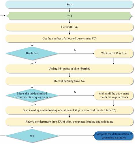
In the proposed E-B&QC model, the dependent variables include the berthing time TB_i of vessel i, the start of loading and unloading operations of vessel i, and the start of departure of vessel i from the channel TE_i. According to the constraints described in Section 3.3, this paper constructs the process of determining the dependent variables based on the berthing and loading and unloading operation processes of container ports. In this paper, MySQL database and Python3.9 are used to determine the above dependent variables. The process of determining dependent variables is as follows:

Step 1 Set i= 1 and proceed to Step 2.

Step 2Consistent with the berthing sequence VO_i, obtain the berth number VB_i of the i ship and the number of bridges assigned to the i ship in turn and then proceed to Step 3.

Step 3In the database query whether vessel i berth VB_i is available, if VB_i is an available berth, go to Step 4, otherwise, proceed to Step 5

Step 4When vessel i berthing, update the berthing status VB_i in the database and record the berthing time TB_i in the database, then proceed to Step 5.

Step 5Vessel i waits at anchor until berth VB_i is free, then vessel i docks at berth VB_i, updates the berth VB_i usage status in the database, and records the vessel berthing time TB_i, then proceed to Step 6.

Step 6Query from the database the number of consecutive free cranes at berth VB_i. If the number meets the scheduled number of loading and unloading cranes VC_i, go to Step 7, otherwise, proceed to Step 8

Step 7Vessel i starts loading and unloading service according to the scheduled plan, records the start time TS_i in the database, and calculates the loading and unloading time VE_i/VC_i*CE₀ according to the loading and unloading efficiency CE₀, the loading and unloading volume VE_i of vessel i and the number of quay cranes VC_i in service, records the vessel departure time TF_i, and updates the use of berth VB_i and quay cranes VC_i after the vessel leaves the port. status after the ship leaves port, and proceed to Step 9.

Step 8Vessel i berths and waits until the number of quay cranes at berth VB_i meets the requirement of VC_i, then vessel i starts the loading and unloading operation service according to the scheduled plan, records the starting loading and unloading time TS_i in the database, and calculates the loading and unloading operation time VE_i/VC_i*CE₀ according to the loading and unloading operation efficiency CE₀, the loading and unloading volume VE_i of vessel i and the number of quay cranes in service VC_i, and records the vessel departure time TF_i. And update the use status of berth VB_i and quay crane VC_i after the ship leaves the port, and proceed to Step 9.

Step 9If i≥ v, then go to Step 11, otherwise, proceed to Step 10

Step 10i = i + 1, then return to Step 2

Step 11Complete the determination of all dependent variables.

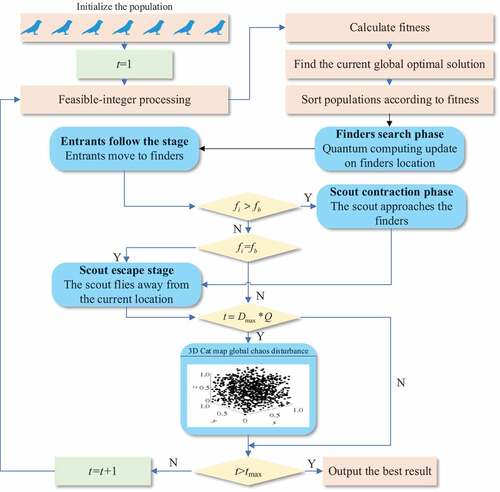
The dependent variable determination process can be shown in Figure 1:

Figure 1. Dependent variable determination flowchart.

In previous studies, the berth-quay crane allocation optimization problem can be solved by linear programming method (Tian and Meng 2018), heuristic algorithm (Jiao et al. 2018), and intelligent optimization algorithm (Cai et al., 2020). Considering that the intelligent optimization algorithm in constrained nonlinear optimization problems has good performance in the solution process, so this paper tries to use the intelligent optimization algorithm to solve the E-B&QC model.

Chaotic Quantum Sparrow Search Algorithm (CQSSA) and E-B&QC Model Solution

The Introduce of the Sparrow Search Algorithm

The Sparrow Search Algorithm (SSA) is an emerging heuristic intelligent optimization algorithm proposed by Xue J, Shen, and Xue (2020) in 2020 inspired by sparrow foraging and anti-predation activities. SSA has been successfully applied in the fields of energy (Liu and Wang 2021; Song W et al. 2020; Yang et al. 2021; Yuan et al. 2021), medical (Liu et al. 2021; OuOuyang, Zhu, and Qiu 2021; Wang, Zhang, and Yang 2021), transportation (Nepomuceno et al. 2019; Sang, Wang, and Yan 2001; Zhang and Ding 2021), computer (Mao and Chen 2005), and economy (Kocarev et al. 1998; Mao, Chen, and Lian 2004) due to its strong local search capability, fast convergence, few control parameters, and simple structure for easy implementation (Xue J, Shen, and Xue 2020). Considering the good performance of the SSA in solving optimization problems, this paper tries to use the SSA for solving the E-B&QC model.

The SSA simulates the foraging behavior of sparrows in nature and divides the sparrow population into finders and entrants, where the finders have better fitness values and provide the foraging direction and foraging area for the population, while the entrants use the conditions provided by the finders to obtain food. Also, there are random scouts within the population, and when they are aware of the danger, they will send out danger signals in time and the whole population will immediately engage in anti-predatory behavior. In this case, the identities of finders and entrants can be switched at any time with the iteration of the algorithm, but the ratio of both remains constant. The basic SSA framework consists of three parts..

(1) Update Finders Location

In the basic SSA, each sparrow represents a solution to the problem with the following individual matrix, as shown in Eq. (23(23) $X=[X_1,X_2...X_i...X_n{]}^T=\left[\begin{array}{ccccc}{x}_{1,1}& x_{1,2}& ...& ...& x_{1,d}\\ x_{1,1}& x_{1,2}& ...& ...& x_{1,d}\\ ⋮& ⋮& ⋮& ⋮& ⋮\\ x_{n,1}& x_{n,2}& ...& ...& x_{n,d}\end{array}\right]$(23) ),

(23) $X=[X_1,X_2...X_i...X_n{]}^T=\left[\begin{array}{ccccc}{x}_{1,1}& x_{1,2}& ...& ...& x_{1,d}\\ x_{1,1}& x_{1,2}& ...& ...& x_{1,d}\\ ⋮& ⋮& ⋮& ⋮& ⋮\\ x_{n,1}& x_{n,2}& ...& ...& x_{n,d}\end{array}\right]$(23)

where N denotes the number of sparrow populations and d represents the dimension of the space to be searched.

Finders with better fitness values in the SSA can be found preferentially in kind. Compared to entrants, finders have the responsibility of finding food and guiding the overall population movement, so finders can then search a wider area. The location of the finder is updated as Eq. (24(24) $X_i^{t+1}=\left\{\begin{array}{c}{X}_i^t\times exp\left(\frac{-i}{\alpha \bullet T_{max}}\right),R_2<ST\\ X_i^t+Q\bullet L\hspace{0.17em},R_2\ge ST\end{array}\right.$(24) ),

(24) $X_i^{t+1}=\left\{\begin{array}{c}{X}_i^t\times exp\left(\frac{-i}{\alpha \bullet T_{max}}\right),R_2<ST\\ X_i^t+Q\bullet L\hspace{0.17em},R_2\ge ST\end{array}\right.$(24)

where t denotes the number of iterations; i = 1, 2, …, N, j = 1, 2, …, d, x_ij denotes the position of the i sparrow individual in the j dimension; the random number of α ∊ (0,1); T_max denotes the maximum number of iterations set by the algorithm; R₂ ∊ (0,1) denotes warning value; ST ∊ (0.5,1) denotes the safety threshold; the matrix of L= [1,1, …,1]_1×d; Q denotes a random number that obeys the N(0,1) distribution; if R₂ < ST, denotes that the foraging environment is safe, finders can continue to search for physical objects; if R₂ ≥ ST, denotes that some of the finders have received an attack and the population needs to be moved quickly to a safe area.

(2) Update entrants location

70–85% of the sparrow population is made up of entrants, which update their position according to the position of the finders. When the finders find food, the entrants leave their current position and fly toward the area where the food was found. The location of Entrants was updated as Eq. (25(25) $X_i^{t+1}=\left\{\begin{array}{cc}Q\cdot exp\left(\frac{X_{worst}-X_i^t}{\alpha T_{max}}\right),& i>\frac{n}{2}\\ X_{best}^{t+1}+\left|X_i^t-X_{best}^{t+1}\right|\cdot A\cdot L,& i\le \frac{n}{2}\end{array}\right.$(25) ),

(25) $X_i^{t+1}=\left\{\begin{array}{cc}Q\cdot exp\left(\frac{X_{worst}-X_i^t}{\alpha T_{max}}\right),& i>\frac{n}{2}\\ X_{best}^{t+1}+\left|X_i^t-X_{best}^{t+1}\right|\cdot A\cdot L,& i\le \frac{n}{2}\end{array}\right.$(25)

where X_best denotes the position of the individual with the best fitness value of the current population, X_worst denotes the position of the individual with the worst fitness value of the current population, and A denotes a d × d matrix, each element of which is randomly assigned as 1 or −1. When i ≤ n/2, it indicates that the NO.i entrant is already foraging near the optimal location, and when i > n/2, it indicates that the entrants with poor individual locations need to go to another location for foraging.

(3) Detection and early warning judgment

In the entire sparrow population, 15%–30% of sparrows have a sense of detection and warning, called scouts. Scouts can be aware of the presence of predators, the mathematical model of this type of scout is shown as Eq. (26(26) $X_i^{t+1}=\left\{\begin{array}{cc}{X}_{best}^t+\beta \left|X_i^t-X_{best}^t\right|,& f_i>f_b\\ X_{best}^{t+1}+K\frac{\left|X_i^t-X_{best}^{t+1}\right|}{\left(f_i-f_w\right)+\epsilon },& f_i=f_b\end{array}\right.$(26) ),

(26) $X_i^{t+1}=\left\{\begin{array}{cc}{X}_{best}^t+\beta \left|X_i^t-X_{best}^t\right|,& f_i>f_b\\ X_{best}^{t+1}+K\frac{\left|X_i^t-X_{best}^{t+1}\right|}{\left(f_i-f_w\right)+\epsilon },& f_i=f_b\end{array}\right.$(26)

where β follows a normal distribution with a variance of 1 and mean of 0. It is called the random step control coefficient; K = [−1,1] is a random number; f_i denotes the fitness value of individual sparrow; f_b is the optimal value of the current population; f_ω is the most inferior value of the current population; ε represents the minimum value to avoid zero division error. When f_i > f_b, it means that the individual sparrow is at the edge of the population and is vulnerable to predators, requiring a contraction operation; When f_i = f_b proves that the scout has become aware of the threat of predators and needs to fly to other individuals, closer to a safe location.

Due to the speed update mechanism in the late evolutionary stage of the SSA refers to the historical speed, it leads to the poor local search ability of the algorithm and a dramatic decrease in population diversity. Moreover, the SSA lacks a mutation mechanism, so it is particularly prone to fall into local optimality, generating the problem of not converging to an optimal solution or even failing to produce valid results. Therefore, the improvement of the SSA focuses on the effective enhancement of population diversity and the significant improvement of the ability of the algorithm to jump out of the local optimum, thus allowing the population to maintain its continuous optimization during the iterative process.

Considering the excellent performance of quantum computing and chaos mapping for swarm intelligence algorithm improvement, this paper tries to improve the SSA based on quantum computing strategy and chaos mapping to improve the solving capability of the SSA for fast and accurate solution of the E-B&QC model.

Firstly, the quantum computing mechanism (QCM) is used to improve the search position of the SSA to improve the global convergence of the algorithm. Secondly, chaotic perturbation is performed using 3D-cat mapping mechanism for poorly adapted individuals to increase the population diversity and thereby make the SSA jump out of the local optimum. Finally, a new hybrid optimization algorithm named CQSSA is proposed for the E-B&QC model solving.

The Design of the Quantum Sparrow Search Algorithm (QSSA)

Considering the problem of poor global convergence of the SSA, this paper improves the SSA based on the QCM and introduces a quantum computing strategy. For improving the SSA, quantum strategy is used to make the foraging behavior of each sparrow have the meaning of quantum probability and improve the global convergence of the algorithm.

In quantum space, the velocity and position of a particle cannot be determined simultaneously. Consequently, the wave function $\beta =\frac{max\left(dt-i\right)}{maxdt}+0.5$ is used to describe the state of the particle, and the probability density function of the particle at a point in space is obtained by solving the Schrödinger equation. Then, the position of the particle is obtained by Monte Carlo simulation according to Eq. (27)(27) $X_{id}^t=P\pm \frac{L}{2}1n\left(1/u\right)$(27) as follows,

(27) $X_{id}^t=P\pm \frac{L}{2}1n\left(1/u\right)$(27)

where u is a random number varying in the range [0,1]; p defined by Eq. (28(28) $p\left(t+1\right)={\phi }_1\times p_i^{dt}+\left(1-{\phi }_2\right)\times p_g^t$(28) ),

(28) $p\left(t+1\right)={\phi }_1\times p_i^{dt}+\left(1-{\phi }_2\right)\times p_g^t$(28)

where d is the size of the particle; φ₁ and φ₂ are random numbers varying in the range; p_i^dt is the current best position of particle i; p^t_g is the historical best position of the particle i.

where L is the range that restricts the individual search of sparrows, and it is defined as Eq. (29(29) $L(t+1)=2\times \beta \times \left|mbest-X_{id}^t\right|$(29) ),

(29) $L(t+1)=2\times \beta \times \left|mbest-X_{id}^t\right|$(29)

where mbest is the average optimal position, which is used to represent the current average optimal solution of all particles, as defined in Eq. (30(30) $mbest=\sum _{i=1}^M{p}_i/M=(\sum _{i=1}^M{p}_{i1}/M,\sum _{i=1}^M{p}_{i2}/M,\dots ,\sum _{i=1}^M{p}_{id}/M)$(30) ),

(30) $mbest=\sum _{i=1}^M{p}_i/M=(\sum _{i=1}^M{p}_{i1}/M,\sum _{i=1}^M{p}_{i2}/M,\dots ,\sum _{i=1}^M{p}_{id}/M)$(30)

where $\beta =\frac{max(dt-i)}{maxdt}+0.5$ is the coefficient of shrinkage and expansion; M is the number of particles; max dt is the maximum number of iterations.

Ultimately, the position of the particle is given by Eq. (31(31) $X_{id}^{t+1}=\left\{\begin{array}{c}P+\beta \times \left|mbest-X_{id}^t\right|\times ln(\mathrm{l}/u)rand\le 0.5\\ P-\beta \times \left|mbest-X_{id}^t\right|\times ln(\mathrm{l}/u)rand>0.5\end{array}\right.$(31) ),

(31) $X_{id}^{t+1}=\left\{\begin{array}{c}P+\beta \times \left|mbest-X_{id}^t\right|\times ln(\mathrm{l}/u)rand\le 0.5\\ P-\beta \times \left|mbest-X_{id}^t\right|\times ln(\mathrm{l}/u)rand>0.5\end{array}\right.$(31)

Considering each finder in the SSA as each particle in the quantum computing strategy, the improved equation for the update of finders in the QSSA is shown in Eq. (32)(32) $X_{id}^{t+1}=p\pm \beta \left|mbest-X_{id}^t\right|*\ln (\text{l}/u),R_{2}ST{X}_{id}^t+Q\cdot L,R_2\ge ST$(32) below,

(32) $X_{id}^{t+1}=p\pm \beta \left|mbest-X_{id}^t\right|*\ln (\text{l}/u),R_{2}ST{X}_{id}^t+Q\cdot L,R_2\ge ST$(32)

The process of the QSSA is described as follows:

Step 1 Set the initial values. The sparrow population is initialized to n. The position of the sparrow i in the initial population is ${X_{id}}^0$; initialize the number of finds, entrants, and scouts. Set the target dimension, etc.

Step 2 Calculate the individual fitness value (I). Calculate the fitness value of each sparrow using the objective function, and update the best and worst positions, update the best and worst fitness values.

Step 3 Update the position of finders (I). The population is ranked according to the superiority of the fitness value, and the finders in the better position are selected and the position is updated using Eq. (32)(32) $X_{id}^{t+1}=p\pm \beta \left|mbest-X_{id}^t\right|*\ln (\text{l}/u),R_{2}ST{X}_{id}^t+Q\cdot L,R_2\ge ST$(32) .

Step 4 Update the entrants’ positions (I). The entrants are selected according to the ratio set in the initialization, and the position is updated using Eq. (25)(25) $X_i^{t+1}=\left\{\begin{array}{cc}Q\cdot exp\left(\frac{X_{worst}-X_i^t}{\alpha T_{max}}\right),& i>\frac{n}{2}\\ X_{best}^{t+1}+\left|X_i^t-X_{best}^{t+1}\right|\cdot A\cdot L,& i\le \frac{n}{2}\end{array}\right.$(25) .

Step 5 Calculate the fitness value (II). Calculate the fitness value, update the best and worst positions, and update the best and worst fitness values.

Step 6 Update the scout position (II). The fitness value of the scout is judged in relation to the population optimum, and the scout position is updated using Eq. (26)(26) $X_i^{t+1}=\left\{\begin{array}{cc}{X}_{best}^t+\beta \left|X_i^t-X_{best}^t\right|,& f_i>f_b\\ X_{best}^{t+1}+K\frac{\left|X_i^t-X_{best}^{t+1}\right|}{\left(f_i-f_w\right)+\epsilon },& f_i=f_b\end{array}\right.$(26) .

Step 7 Stop state test. If the number of iterations has been reached, continue to step 8; otherwise, return to Step 2.

Step 8 Final stage. At the end of the algorithm, the experimental data are exported, analyzed, and processed.

The pseudo-code of the CSSA is shown in Figure 2.

Figure 2. Pseudo-code of QSSA.

The Design of the Chaotic Sparrow Search Algorithm (CSSA)

Chaotic distributions have similar but different randomness properties compared to uniform and Gaussian distributions (Kocarev et al. 1998; Li and Zheng 2002; Mao and Chen 2005; Mao, Chen, and Lian 2004) and thus can exhibit random behavior without any random factors. Many properties of chaos can be applied to improve optimization computations. Some researches have shown that the stochastic nature of chaos can make the search jump out of the current optimal point and thus prevent the iterative search from falling into a local optimum (Li et al. 2017). Especially, when the parameters of chaos are chosen by a large number of measurements, the ergodic nature of chaos makes its final solution approximate the true optimal solution at arbitrary accuracy. Although the random numbers generated by chaotic perturbations cannot support the algorithm to complete an ergodic search in the space of continuous variables, chaotic variables are feasible within the accuracy that a computer can represent. Chaos is commonly used in random number generators (Nepomuceno et al. 2019; Sang, Wang, and Yan 2001). Song W et al. (2020) first introduced chaos into the SSA to optimize the initial state of the population and to increase population diversity by jumping out of the local optimal point at the late stage of evolution. Zhang and Ding (2021) proposed an optimal stochastic configuration network CSSA-SCN based on chaotic sparrow search algorithm by introducing logistic mapping, adaptive hyperparameters, and variational operators in the SSA to improve the global search capability of the algorithm.

Currently, Logistic, Tent, An, and Cat mapping functions are commonly used as chaotic sequence generators. Li, Hong, and Kang (2013) analyzed the chaotic properties of these four mapping functions. The results show that the distribution of Cat mapping functions is relatively uniform during the iterative process, and there is no cyclic phenomenon. The chaotic sequence values of the Cat mapping function can be taken as 0 and 1. Therefore, the Cat mapping function has better chaotic distribution properties and can improve the population diversity. Hence, an improved Cat mapping function to improve the Lyapunov exponent is used and introduced into the SSA to achieve satisfactory performance.

The iterative form of the standard two-dimensional Cat mapping function (based on two dimensions) is defined by Eq. (33(33) $\left\{\begin{array}{cc}{x}_{n+1}=\left(x_n+y_n\right)& \mathrm{m}\mathrm{o}\mathrm{d}1\\ y_{n+1}=\left(x_n+2y_n\right)& \mathrm{m}\mathrm{o}\mathrm{d}1\end{array}\right.$(33) ),

(33) $\left\{\begin{array}{cc}{x}_{n+1}=\left(x_n+y_n\right)& \mathrm{m}\mathrm{o}\mathrm{d}1\\ y_{n+1}=\left(x_n+2y_n\right)& \mathrm{m}\mathrm{o}\mathrm{d}1\end{array}\right.$(33)

Equation (33)(33) $\left\{\begin{array}{cc}{x}_{n+1}=\left(x_n+y_n\right)& \mathrm{m}\mathrm{o}\mathrm{d}1\\ y_{n+1}=\left(x_n+2y_n\right)& \mathrm{m}\mathrm{o}\mathrm{d}1\end{array}\right.$(33) is usually expressed in matrix form as Eq. (34(34) $\left[\begin{array}{c}{x}_{n+1}\\ y_{n+1}\end{array}\right]=\left[\begin{array}{c}1\\ 1\end{array}\begin{array}{c}1\\ 2\end{array}\right]\left[\begin{array}{c}{x}_n\\ y_n\end{array}\right]\mathrm{m}\mathrm{o}\mathrm{d}1$(34) ),

(34) $\left[\begin{array}{c}{x}_{n+1}\\ y_{n+1}\end{array}\right]=\left[\begin{array}{c}1\\ 1\end{array}\begin{array}{c}1\\ 2\end{array}\right]\left[\begin{array}{c}{x}_n\\ y_n\end{array}\right]\mathrm{m}\mathrm{o}\mathrm{d}1$(34)

where the operation of the “mod 1” takes the fractional part of a real number. Eigenvalues of the coefficient matrix of the Cat mapping function are σ₁ = 2.618 > 1 and σ₂ = 0.382 < 1. Therefore, the resulting maximum Lyapunov exponent of the Cat mapping function is λ₁ = ln2.618 > 0. The larger the positive Lyapunov exponent, the faster the orbit separation, and thus the more complex the 3D cat mapping function becomes, the better the chaotic performance. However, after a finite number of iterations, the discretized cat mapping function exhibits the phenomenon of Poincare recovery. To solve this problem more efficiently, Li, Hong, and Kang (2013) extended the two-dimensional cat mapping function to a three-dimensional cat mapping function. The main idea is to introduce two parameters, a and b, into the two-dimensional cat mapping function, as shown in Eq. (35)(35) $\left[\begin{array}{c}{x}_{n+1}\\ y_{n+1}\end{array}\right]=\left[\begin{array}{cc}1& a\\ b& ab+1\end{array}\right]\left[\begin{array}{c}{x}_n\\ y_n\end{array}\right]\mathrm{m}\mathrm{o}\mathrm{d}1$(35) .

(35) $\left[\begin{array}{c}{x}_{n+1}\\ y_{n+1}\end{array}\right]=\left[\begin{array}{cc}1& a\\ b& ab+1\end{array}\right]\left[\begin{array}{c}{x}_n\\ y_n\end{array}\right]\mathrm{m}\mathrm{o}\mathrm{d}1$(35)

On the basis, set x_n,y_n and z_n constant; Then, the definition of the 3D cat mapping function can be obtained by implementing the 2D cat mapping function on the three interaction planes (yz, xz, xy) and connecting the three associated equations, as shown in Eq. (36(36) $\left[\begin{array}{c}{x}_{n+1}\\ y_{n+1}\\ z_{n+1}\end{array}\right]=A\left[\begin{array}{c}{x}_n\\ y_n\\ z_n\end{array}\right]\mathrm{m}\mathrm{o}\mathrm{d}1$(36) ),

(36) $\left[\begin{array}{c}{x}_{n+1}\\ y_{n+1}\\ z_{n+1}\end{array}\right]=A\left[\begin{array}{c}{x}_n\\ y_n\\ z_n\end{array}\right]\mathrm{m}\mathrm{o}\mathrm{d}1$(36)

where A is the product of the coefficient matrices from the three planes when the cat mapping is completed.

According to Eq. (36(36) $\left[\begin{array}{c}{x}_{n+1}\\ y_{n+1}\\ z_{n+1}\end{array}\right]=A\left[\begin{array}{c}{x}_n\\ y_n\\ z_n\end{array}\right]\mathrm{m}\mathrm{o}\mathrm{d}1$(36) ), the phase space of x_n,y_n and z_n is restricted to the unit cube, whose form in the final iteration is given by Eq. (37(37) $\left[\begin{array}{c}{x}_{n+1}\\ y_{n+1}\\ z_{n+1}\end{array}\right]=\left[\begin{array}{ccc}1+a_x{a}_z{b}_y& a_z& a_y+a_x{a}_z+a_x{a}_y{a}_z{b}_y\\ b_z+a_x{b}_y+a_x{a}_z{b}_y{b}_z& a_z{b}_z+1& a_y{b}_z+a_x{a}_y{a}_z{b}_y{b}_z+a_x{a}_z{b}_z+a_x{a}_y{b}_y+a_x\\ a_x{b}_x{b}_y+b_y& b_x& a_x{a}_y{b}_x{b}_y+a_x{b}_x+a_y{b}_y+1\end{array}\right]\left[\begin{array}{c}{x}_n\\ y_n\\ z_n\end{array}\right]\mathrm{m}\mathrm{o}\mathrm{d}1$(37) )

(37) $\left[\begin{array}{c}{x}_{n+1}\\ y_{n+1}\\ z_{n+1}\end{array}\right]=\left[\begin{array}{ccc}1+a_x{a}_z{b}_y& a_z& a_y+a_x{a}_z+a_x{a}_y{a}_z{b}_y\\ b_z+a_x{b}_y+a_x{a}_z{b}_y{b}_z& a_z{b}_z+1& a_y{b}_z+a_x{a}_y{a}_z{b}_y{b}_z+a_x{a}_z{b}_z+a_x{a}_y{b}_y+a_x\\ a_x{b}_x{b}_y+b_y& b_x& a_x{a}_y{b}_x{b}_y+a_x{b}_x+a_y{b}_y+1\end{array}\right]\left[\begin{array}{c}{x}_n\\ y_n\\ z_n\end{array}\right]\mathrm{m}\mathrm{o}\mathrm{d}1$(37)

The matrix of the coefficients is shown as Eq. (38(38) $A=\left[\begin{array}{ccc}2& 1& 3\\ 3& 2& 5\\ 2& 1& 4\end{array}\right]$(38) ),

(38) $A=\left[\begin{array}{ccc}2& 1& 3\\ 3& 2& 5\\ 2& 1& 4\end{array}\right]$(38)

By calculating three eigenvalues, σ₁ = 7.1842 > 1, σ₂ = 0.2430 < 1, and σ₃ = 0.5728 < 1, the corresponding Lyapunov indices were obtained:λ₁ = ln2.618 > 0, λ₂ = ln0.243 < 0, λ₃ = ln0.5728 < 0.

The calculation results show that the maximum eigenvalue of the 3D cat mapping function exceeds the maximum eigenvalue of the 2D cat mapping function, and its corresponding maximum Lyapunov exponent also exceeds the maximum Lyapunov exponent of the 2D cat mapping function.

The process of the CSSA is described as follows:

Step 1 Set the initial values. The sparrow population is initialized as n; the position of the sparrow i in the initial population is $X_{id}^0$; initialize the number of finders, entrants, and scouts; set the target dimension X, the perturbation generation ratio Q, the mixing ratio R, and the number of iterations Dmax, etc.

Step 2 Calculate the individual fitness value (I). Calculate the fitness value of each sparrow using the objective function, and update the optimal and worst positions, and update the optimal and worst fitness values.

Step 3 Update the position of the finders. The populations are ranked according to the superiority of the fitness values, and the finds with the better positions are selected and the positions are updated using Eq. (24)(24) $X_i^{t+1}=\left\{\begin{array}{c}{X}_i^t\times exp\left(\frac{-i}{\alpha \bullet T_{max}}\right),R_2<ST\\ X_i^t+Q\bullet L\hspace{0.17em},R_2\ge ST\end{array}\right.$(24) .

Step 4 Update the positions of entrants. The entrants are selected according to the ratio set in the initialization, and the position is updated using Eq. (25)(25) $X_i^{t+1}=\left\{\begin{array}{cc}Q\cdot exp\left(\frac{X_{worst}-X_i^t}{\alpha T_{max}}\right),& i>\frac{n}{2}\\ X_{best}^{t+1}+\left|X_i^t-X_{best}^{t+1}\right|\cdot A\cdot L,& i\le \frac{n}{2}\end{array}\right.$(25) .

Step 5 Calculate the fitness value (II). Calculate the fitness value, update the best and worst positions, and update the best and worst fitness values.

Step 6 Update the scout position. The fitness value of the scout is judged concerning the population optimum, and the scout position is updated using Eq. (26)(26) $X_i^{t+1}=\left\{\begin{array}{cc}{X}_{best}^t+\beta \left|X_i^t-X_{best}^t\right|,& f_i>f_b\\ X_{best}^{t+1}+K\frac{\left|X_i^t-X_{best}^{t+1}\right|}{\left(f_i-f_w\right)+\epsilon },& f_i=f_b\end{array}\right.$(26) .

Step 7 Determine the number of iterations. If the number of iterations Dmax*Q has been reached, continue to step 8; Otherwise, return to step 9.

Step 8 Population perturbation. The current population fitness values are ranked, and the worse individuals with fitness values in the bottom R% are selected and their current positions are perturbed using Eq. (37)(37) $\left[\begin{array}{c}{x}_{n+1}\\ y_{n+1}\\ z_{n+1}\end{array}\right]=\left[\begin{array}{ccc}1+a_x{a}_z{b}_y& a_z& a_y+a_x{a}_z+a_x{a}_y{a}_z{b}_y\\ b_z+a_x{b}_y+a_x{a}_z{b}_y{b}_z& a_z{b}_z+1& a_y{b}_z+a_x{a}_y{a}_z{b}_y{b}_z+a_x{a}_z{b}_z+a_x{a}_y{b}_y+a_x\\ a_x{b}_x{b}_y+b_y& b_x& a_x{a}_y{b}_x{b}_y+a_x{b}_x+a_y{b}_y+1\end{array}\right]\left[\begin{array}{c}{x}_n\\ y_n\\ z_n\end{array}\right]\mathrm{m}\mathrm{o}\mathrm{d}1$(37) .

Step 9 Stop state test. If the maximum number of iterations is reached, proceed to Step 10; otherwise, return to Step 2.

Step 10 Final stage. At the end of the algorithm, the experimental data are exported, analyzed, and processed

The pseudo-code of the CSSA is shown in Figure 3.

Figure 3. Pseudo-code of CSSA.

The Formulate of the Coding Rules for Individual Sparrows for the E-B&QC Model

Based on the optimization variables of the E-B&QC model, the coding rules applicable to the E-B&QC model and the CQSSA are developed. In this paper, it is stipulated that a stock individual is an independent matrix, the number of rows of the matrix is determined by the ship berthing order, ship berthing position, and the number of quay cranes assigned to the ship, which are three rows of the coding matrix, and the number of columns of the matrix is determined by the number of ships arriving at the port. Since the order of berthing, berthing position and the number of assigned quay cranes are all-natural numbers, each item in the matrix is coded as a natural number. Table 3 gives an example of the coding method for the population individuals, and the first column is used as an example to introduce the coding method: the first ship, the berthing order (VO) is 3, the berthing position number (VB) is 1, and the number of assigned bridges (VC) is 3.

Table 3. The example of the sparrow code matrix

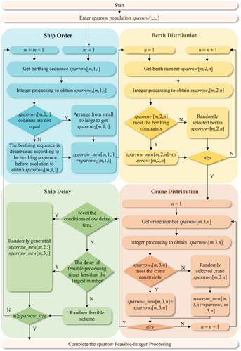
The Design of the Sparrow Feasible-Integer Processing Algorithm (SF-IPA)

The optimization objectives are natural numbers in the actual berth-quay crane optimization process, but the optimization variables are real numbers in the evolutionary process of the sparrow algorithm. Therefore, the sparrow feasible-integer processing algorithm (SF-IPA) is designed to perform a feasible-integer of the values of the population individual encoding matrix. In the process of the E-B&QC model solution based on the CQSSA, the coding matrix obtained by evolution is a real number matrix, and based on the SF-IPA, the coding matrix is integrated to obtain the natural number matrix. The SF-IPA is designed as follows.

Step 1: Let m = 1; proceed to Step 2.

(1) Feasible integer processing module for ship order sparrow[m,1,:] of sparrow m

Step 2: Arrange m the first row of sparrow[m,1,:] of sparrow m from smallest to largest to get sparrow₁[m,1,:]. If the values in sparrow₁[m,1,:] are equal, go to Step 3, otherwise, go to Step 4.

Step 3: Order sparrow₁[m,1,:] by the size of the ship corresponding to the value, the order of arrangement as each ship berthing order sparrow₂[m,1,:], so that sparrow_new[m,1,:] = sparrow₂[m,1,:], proceed to Step 5;

Step 4: For ships with equal values in sparrow₁[m,1,:], determine the ship berthing order sparrow₂[m,1,:] in the evolved individual by referring to the last iteration of ship berthing order so that sparrow_new[m,1,:] = sparrow₂[m,1,:], and move to Step 5.

(2) The ship order sparrow[m,2,:] of sparrow m feasible-integer processing module

Step 5: Let n = 1, proceed to Step 6;

Step 6: Round the value of berthing berth sparrow[m,2,n] of the ship n in sparrow m to get sparrow₁[m,2,n], if the berthing constraint of ship n is satisfied, make sparrow_new[m,2,n] = sparrow₁[m,2,n], otherwise, under the berthing constraint of ship n, randomly select berthing sparrow₂[m,2,n], so that sparrow_new[m,2,n] = sparrow₂[m,2,n], and proceed to Step 7;

Step 7: If n≥ v, proceed to Step 9, otherwise proceed to Step 8;

Step 8: Let n= n+ 1, proceed to Step 6;

(3) The number of quay cranes assigned to the ships sparrow[m,3,:] of sparrow m feasible-integer processing module

Step 9: Make n= 1, proceed to Step 10.

Step10: Round the value of sparrow[m,3,n], the assigned number of quay cranes of the ship n in sparrow m, to get sparrow₁[m,3,n], then if sparrow₁[m,3,n] satisfies the quay crane constraint of ship n, make sparrow_new[m,3,n] = sparrow₁[m,3,n], otherwise, randomly form sparrow₂[m,3,n] under the constraint of the number of quay cranes of ship n, so that sparrow_new[m,3,n] = sparrow₂[m,3,n], proceed to Step 11.

Step 11: If n≥ v, proceed to Step 13, otherwise proceed to Step 12;

Step 12: Let n= n+ 1, proceed to Step 10;

(4) The ship delay feasibility processing module of Sparrow m

Step 13: Calculate the remaining dependent variables according to the allocation scheme corresponding to sparrow m. If each vessel delay satisfies its delay constraint (18), move to Step 15, otherwise proceed to Step 14.

Step 14: If the number of ship delay feasibility treatments of sparrow m is less than the maximum number of delay feasibility treatments, then randomly assign berthing sparrow_new[m,2,:] and quay crane sparrow_new[m,3,:] when the ship berthing constraints and quay crane constraints are satisfied, otherwise, randomly select the existing feasible population individuals as the allocation scheme for this iteration of sparrow m the allocation scheme to Step 13.

Step 15: If m≥ sparrow_new, move to Step17, otherwise move to Step16;

Step16 Let m= m+ 1, proceed to Step2;

Step17: Complete the feasible-integer process for sparrows with population size sparrow_size.

The flow chart of the feasible-integer module is shown in Figure 4.

Figure 4. The flowchart of sparrow feasible-integer processing algorithm (SF-IPA).

The Design of the E-B&QC Model Solving Process Based on the CQSSA

Combined with the E-B&QC model proposed in this paper and the improved CQSSA, this paper provides a new solution method for the E-B&QC model based on CQSSA, which provides a better solution for container port berth-quay crane scheduling.

The pseudo-code of the CQSSA-based E-B&QC model solving process is shown in Figure 5.

Figure 5. Pseudo-code of CQSSA-based E-B&QC model solving process.

The flowchart is shown in Figure 6

Figure 6. Flow chart of the CQSSA for solving the E-B&QC model.

Rolling Optimization Mechanism

To better apply the E-B&QC-CQSSA solution method proposed in this paper to the actual container port, this paper proposes a rescheduling optimization scheme suitable for the E-B&QC-CQSSA solution method to meet the scheduling requirements. Due to the complicated meteorological and tidal factors at sea, ships may not arrive at the port at the planned time. Based on the principle of “arrival-assignment,” the E-B&QC model develops a rolling optimization mechanism to optimize berth-crane for arriving vessels. When a group of vessels arrives in port, they enter the berth-quay crane optimization sequence. After the next batch of vessels arrives at the port, they enter the new berth-quay crane optimization sequence, and for the vessels that did not enter the port in the previous round, they join the next sequence and continue the optimization allocation. According to this process, the berth-quay crane optimization process for all vessels is completed.

Numerical Experiment and Result Analysis

The Simulation Research

A small river port in southern China and a medium-sized river port in northern China are used as examples to test the feasibility and superiority of the berth-quay crane allocation method established in this paper. For a small river port in the south, this paper conducts a simulation study with 5 arriving ships as a formation. Among them, three are small and medium-sized ships and two are large ships. The number of berths where ships dock is 4, berths 1–3 are 300 m in length with a draft of 15 m, berth 4 is 300 m in length with a draft of 20 m, and the number of quay cranes is 10. Due to the limitation of ship length and draught depth, only berth 4 is available for berthing large ships, while all berths can berth small and medium-sized ships. Up to two loading/unloading cranes can be operated simultaneously for small and medium-sized vessels, and up to three loading/unloading cranes can be operated simultaneously for large vessels. The loading and unloading operation efficiency of the quay crane is 35 TEU/(unit·h), and the maximum acceptable waiting time for the vessel is 6 hours. For a medium-sized river port in the north, this paper conducts a simulation study with 15 arriving ships as a formation. Among them, 11 are small and medium-sized ships and 4 are large ships. The number of berths in the port is 8. Berths 1, 2, 3, 5, 6, and 7 have a length of 350 m and a draft of 25 m, while berths 4 and 8 have a length of 400 m and a draft of 30 m, and the number of cranes is 20. Due to the limitation of the length and draft of the ships, only berths 4 and 8 are available for berthing large ships, while all berths are available for berthing small and medium-sized ships. Small and medium-sized ships can have up to 2 loading/unloading cranes operating at the same time, and large ships can have up to 3 loading/unloading cranes operating at the same time. The loading and unloading efficiency of the crane is 35 TEU/(unit·h), and the maximum acceptable waiting time for the ship is 8 hours.

This paper creates a dynamic database using MySQL and uses Python 3.9 for programming. The running environment is an Inter(R) Core(TM) i7-7700 CPU @ 3.60 GHz, 3.60 GHz, 8.00GB RAM PC, OS: Windows 10.

Analysis of Model Performance under Different Requirements

In this paper, the E-B&QC model is established to make improvements to the container port berth-quay crane optimization problem mainly from the economic point of view. The purpose of dynamically setting the preference weight coefficients is that the generalization performance of the model can be improved according to the actual situation of container port operations. In the E-B&QC model, the objective functions are considered from the following three aspects: the cost of the shipowner and the port, the economic and environmental cost of the port operation, and the time and economic cost of the shipowner. According to the measured data of a small port in southern China and a medium-sized port in northern China, three different working conditions are designed, and at the same time, the E-B&QC allocation model is applied to two different sizes of ports by setting different preference weights coefficients and conducting simulation tests to obtain different schemes to test whether the allocation scheme under different demands can be achieved by adjusting the preference weights. In order to test the influence of the weight coefficient in the E-B&QC model on the scheduling scheme, this paper takes three common working conditions as examples to conduct simulation experiments. When applying the E-B&QC model, the value of the weight coefficient should be determined according to the actual needs of the port. The three common conditions are as follows:

Application Scenario 1: In the case of regular container port operations, the interests of the shipowner and the port need to be considered

In the case of regular container port operations, the interests between container ports and shipowners need to be considered in a comprehensive manner. At this time, the formulation of the scheme should be based on the principle of improving the efficiency of container port handling operations and reducing the time of the ship in port, which can be achieved by increasing the value of the weight ω₁ to improve the interests of the ship and the port at the same time.

Application Scenario 2: In the peak season of container ports, it is necessary to reduce the cost of additional transport distance for land-based container trucks in the port area and improve the benefits of container ports

During the peak season of container port operation, the cost of container port operation needs to be controlled to obtain more benefits. At this time, the scheme development should be based on the principle of reducing the extra transportation cost of container trucks in the land area of the port and increasing the benefits of the container port, which can be achieved by increasing the value of the weight ω₂ to increase the benefits of the container port.

Application Scenario 3: In the off-season of container ports, it is necessary to improve the interests of shipowners and attract more ships to operate in the port

During the low season of container port operation, the need to improve the interests of shipowners and to attract more other ships to operate in the port. At this time, the program development should be based on the principle of reducing the extra waiting time of container port ships, and the purpose of improving the interests of shipowners can be achieved by increasing the value of the weight ω₃.

According to the application situations, this paper sets up a table of weight coefficients taking values as in Table 4, with the purpose of testing whether the suitable solutions for different situations can be obtained by adjusting the weights ω₁, ω_2, and ω₃.

Table 4. Table of weighting values for E-B&QC model

	ω1	ω2	ω3
Application Scenario 1:Focus on reducing vessel operating time in port	0.5	0.25	0.25
Application Scenario 2: Focus on reducing additional transportation costs for land-based trucks in the port area	0.25	0.5	0.25
Application Scenario 3: Focus on reducing the cost of extra waiting time for ships	0.25	0.25	0.5

Simulation Calculations Applied to Small Ports

In this paper, the study of simulation calculation is carried out in a small river port in southern China as an example. The scheduling scheme under three scenarios is shown in Table 4, and the corresponding objective function values are shown in Table 5.

Table 5. Scheduling arrangements for three scenarios in a small river port in southern China

Vessel serial number		1	2	3	4	5
Application Scenario 1	Inbound order	1	3	5	4	2
	Berthing position	3	2	1	4	4
	Number of quay crane	2	2	3	3	3
Application Scenario 2	Inbound order	1	5	4	3	2
	Berthing position	2	3	1	4	4
	Number of quay crane	2	1	3	3	3
Application Scenario 3	Inbound order	1	2	4	5	3
	Berthing position	1	2	3	4	4
	Number of quay crane	3	2	2	3	3

From Tables 5 and 6, it can be seen that for increasing the value of ω₁, the time of the ships in port in the first case is reduced by 0.36 hours or 4.65% in small container ports compared to the second application case. Compared with the third application case, the shipping time in port in the second scenario is reduced by 0.18 hours or 2.38%. From the above results, it can be illustrated that the allocation scheme obtained by appropriately increasing the value of ω₁ can reduce the cost of in-port operation time for small ports and maximize the benefits of container ports and shipowners at the same time.

Table 6. Objective function values for three scenarios of a small river port in southern China

	Vessel operating time in port F1	Additional transportation costs for land-based collector trucks in the port area F2	Additional waiting time costs for ships F3
Application Scenario 1	7.39	1000	11.37
Application Scenario 2	7.75	0	11.57
Application Scenario 3	7.57	800	11.10

In the case of increasing the value of ω₂, in small container ports, compared to the first application case, the additional transport distance of the container truck in the second case is reduced by 1000 m, from 1000 m to 0 m. Compared with the third application case, the additional transport distance of the collector truck in the first case is reduced by 800 m, from 800 m to 0 m. From the above data, it can be illustrated that the allocation scheme obtained by appropriately increasing the value of ω₂ can reduce the container truck transportation cost and make the container port container truck transportation distance shorter in small ports, which in turn reduces the additional transportation cost of a container truck in the land area of the container port.

In the case of increasing the value of ω₃, the cost of extra vessel waiting time is reduced by 2.37%, from 11.37 to 11.10 in small container ports compared to the first application case, and by 4.06%, from 11.57 to 11.10 compared to the second case. From the above data, it can be shown that the allocation scheme obtained by appropriately increasing the value of ω₃ can reduce the cost of extra waiting time for small port vessels, maximize the interests of shipowners and improve customer satisfaction.

Simulation Calculations Applied to Medium-sized Ports

In this paper, a medium-sized river port in north China is used as an example to carry out a simulation calculation study. The scheduling schemes for the three scenarios are shown in Tables 7 and 8, and the corresponding objective functions take the values shown in Table 9.

Table 7. No. 1–8 vessel scheduling arrangement for three scenarios in a medium-sized river port in northern China

Vessel Serial Number		1	2	3	4	5	6	7	8
Application Scenario 1	Inbound sequence	1	2	15	5	10	8	7	3
	Berthing position	3	3	1	7	6	6	6	2
	Number of quay crane	1	3	3	3	2	3	2	1
Application Scenario 2	Inbound sequence	4	3	14	10	2	15	11	6
	Berthing position	2	3	3	7	6	6	7	2
	Number of quay crane	2	1	1	1	1	1	2	3
Application Scenario 3	Inbound sequence	3	4	8	5	15	1	9	10
	Berthing position	3	4	2	7	6	6	7	2
	Number of quay crane	2	3	2	2	3	3	3	1

Table 8. No. 9–15 vessel scheduling arrangement for three scenarios in a medium-sized river port in northern China

Vessel Serial Number		9	10	11	12	13	14	15
Application Scenario 1	Inbound sequence	13	6	9	11	4	14	12
	Berthing position	2	1	1	4	4	3	3
	Number of quay crane	2	2	2	2	2	2	1
Application Scenario 2	Inbound sequence	5	9	12	13	8	6	1
	Berthing position	1	1	2	4	3	4	3
	Number of quay crane	3	1	1	1	3	1	2
Application Scenario 3	Inbound sequence	7	6	13	11	14	2	12
	Berthing position	1	2	1	4	2	4	4
	Number of quay crane	1	2	2	1	1	2	1

Table 9. Objective function values for three scenarios of a medium-sized river port in northern China

	Vessel operating time in port F1	Additional transportation costs for land-based collector trucks in the port area F2	Additional waiting time costs for ships F3
Application Scenario 1	7.55	93333.33	1934.06
Application Scenario 2	10.77	91666.67	1994.62
Application Scenario 3	9.08	95666.67	1851.06

As can be seen from Tables 7–9, in the case of increasing the value of ω₁, the time of the ship in port in the first case is reduced by 3.22 hours, or 29.90%, compared with the second application case, in medium-sized container ports. Compared with the third application scenario, the shipping time in port in the second scenario is reduced by 1.53 hours, or 16.85%, which shows that the allocation scheme of increasing the value of ω₁ in medium-sized ports can reduce the shipping time in port in container ports.

In the case of increasing the value of ω₂, the additional transport distance of the container truck in the second case is reduced from 93,333.33 m to 91,666.67 m, or 1,666.66 m, in comparison with the first application case, in medium-sized container ports. In comparison with the third application scenario, the additional transport distance for trucks in the first scenario is reduced from 95,666.67 m to 91,666.67 m, a reduction of 4,000 m. It can be illustrated that the transport distance for trucks in medium-sized ports can be reduced by increasing the distribution scheme for the value of ω_2.

In the case of increasing the value of ω₃, the cost of extra vessel waiting time is reduced by 4.29% from 1,934.06 to 1,851.06 in the medium-sized container port compared to the first application case, and by 7.20% from 1,994.62 to 1,851.06 compared to the second case. From the above comparative analysis, it can be shown that the allocation scheme of increasing the value of ω₃ in medium-sized ports can reduce the cost of extra waiting time for ships.

Comparative Analysis of Simulation Calculations for Small and Medium-sized Ports

The simulation calculation results of medium-sized ports and small ports are compared and analyzed, and the comparison results are shown as follows.

It can be seen from Table 10 that the E-B&QC model can reduce the ship operating time in port by 4.65% when applied to small ports and by 29.90% when applied to medium ports when compared with the second case by increasing the value of ω₁. In comparison with the third case, the E-B&QC model applied to small ports can reduce the vessel operating time in port by 2.38%, while applied to medium ports can reduce the vessel operating time in port by 16.85%. In the case of increasing the value of ω₂, compared with the first case, the E-B&QC model applied to a small port can only reduce the additional distance traveled by a container truck by 1000 m, while applied to a medium-sized port can reduce the additional distance traveled by a container truck in the land area of the port by 1,666.66 m. In comparison with the third case, the E-B&QC model applied to a small port can only reduce the cost of additional distance traveled by a container truck by 800 m, while applied to a medium-sized port can reduce the cost of additional distance traveled by a container truck by 4,000 m. In the case of increasing the value of ω₃, the E-B&QC model, when compared with the first case, can reduce the cost of extra vessel waiting time by only 2.37% when applied to small ports, and by 4.29% when applied to medium-sized ports. In comparison with the second case, the E-B&QC model applied to small ports can only reduce the cost of extra vessel waiting time by 4.06%, while applied to medium-sized ports can reduce the cost of extra vessel waiting time by 7.20%.

Table 10. Comparison analysis of simulation calculation results for medium-sized ports and small ports

	Application Scenario 1		Application Scenario 2		Application Scenario 3
	Compared with Scenario 2	Compared with Scenario 3	Compared with Scenario 1	Compared with Scenario 3	Compared with Scenario 1	Compared with Scenario 2
Small port	Reduce 4.65%	Reduce 2.38%	Reduce 1000 m	Reduce 800 m	Reduce 2.37%	Reduce 4.06%
Medium-sized port	Reduce 29.90%	Reduce 16.85%	Reduce 1666.66 m	Reduce 4000 m	Reduce 4.29%	Reduce 7.20%

From the above comparative analysis, it can be illustrated that: the larger the scale of the container port, the more complex the loading and unloading operation process, the more obvious the effect of applying the E-B&QC model for logistics optimization of the container port, and a more high-quality solution can be obtained.

However, in the calculation process, it shows the limitation of the scheduling method. When the port scale is small, the berth-quay crane joint scheduling method proposed in this paper can complete the optimization calculation and provide a relatively high-quality solution for container ports in a limited optimization time. With the gradual increase of the port scale, the number of ships that need to be optimized gradually increases. During the optimization calculation process, the optimization dimension increases, which leads to an increase in the time-consuming of the algorithm update iteration process, which in turn reduces the calculation speed. However, through the actual calculation of medium-sized container ports, the extra time is acceptable compared to getting a better solution.

Detailed Scheduling Scheme Display Example

Considering the clear display of the scheduling scheme, the paper takes a small container port as an example, draws a Gantt chart for the scheduling scheme of the container port, and provides a more detailed scheduling scheme, to better show the difference of the scheduling scheme when the value of ω is different. Figure 7 takes the scheduling scheme in Table 5 as an example, and draws three Gantt charts as follows:

Figure 7. Detailed scheduling scheme gantt chart a) Application scenario 1 scheduling scheme gantt chart b) Application scenario 2 scheduling scheme gantt chart c) Application scenario 3 scheduling scheme gantt chart.

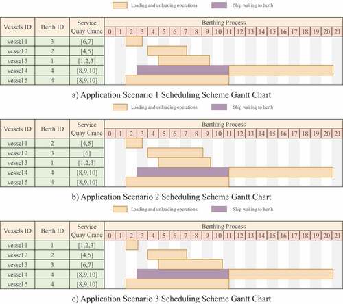
The Gantt chart shows the comparison scheme of three application scenarios. The left side of the figure shows the berth number and the service quay crane number of the berthing ship respectively. The right side of the figure shows the departure process starting from a certain timing zero, the ship loading and unloading operation time, anchorage waiting time, and ship loading and unloading operation. Among them, orange represents loading and unloading operation time, and purple represents anchorage waiting time. For ease of understanding, this paper takes Ship 4 in Application Scenario 1 as an example to illustrate: The berth of Ship 4 is Berth No. 4, the No. 8, No. 9 and No. 10 quay cranes perform loading and unloading operations. The ship enters the port at time 3, waits at the anchorage for 8.54 hours, starts loading and unloading operations at time 11.54, and leaves the container port at time 21.02.

It can be seen from Figure 7 that the above three cases obtain different solutions due to different values of ω, and then obtain different scheduling arrangements and obtain different values of the objective function.

Performance Analysis for CQSSA

To test the feasibility and superiority of the CQSSA proposed in this paper in solving the E-B&QC model, GA (Jiao et al. 2020), PSO (Li et al. 2017), SSA (Xue J, Shen, and Xue 2020), CSSA, and QSSA are selected as comparative algorithms to conduct a comparative study of the model.

Optimize Performance Analysis

In this paper, a comparative study of the solution performance is carried out using the measured data of a small port as an example. Considering that the choice of parameters of each algorithm affects the preferred performance of each algorithm, this paper determines the parameters of the selected algorithm by trial calculation, and the values of each algorithm parameter are shown in Table 11.

Table 11. Parameter selection table for each algorithm

Name of algorithm	Population size	Maximum number of iterations	Other additional parameters
GA (Jiao et al. 2020)	50	100	Crossover probability pc = 0.18	Mutation probability pm = 0.10
PSO (Li et al. 2017)	50	100	c1 = 2.0	c2 = 2.0
SSA (Xue J, Shen, and Xue 2020)	50	100	–
CSSA	50	100	–
QSSA	50	100	–
CQSSA	50	100	–

In this paper, the above six algorithms were used to solve the model 10 times randomly, and the average value of the optimal solution of the model was obtained as shown in Tables 12 and 13, and the average value of the objective function is shown in Table 14.

Table 12. Comparison results of the mean values of 1–5 optimal solutions of six algorithms

Experiment (100 generations of evolution)		1	2	3	4	5
Vessel in port time F1(h)	GA (Jiao et al. 2020)	8.15	8.58	7.87	8.34	7.87
	PSO (Li et al. 2017)	8.01	7.98	8.21	8.19	8.31
	SSA (Xue J, Shen, and Xue 2020)	7.96	7.78	7.47	7.95	7.75
	CSSA	7.69	7.75	7.75	7.75	7.47
	QSSA	7.47	7.47	7.47	7.69	7.75
	CQSSA	7.47	7.75	7.75	7.47	7.47
Additional transportation distance cost for collector trucks F2(m)	GA (Jiao et al. 2020)	14000	0	0	17000	0
	PSO (Li et al. 2017)	14000	0	20000	0	0
	SSA (Xue J, Shen, and Xue 2020)	0	0	0	0	6000
	CSSA	0	0	0	0	0
	QSSA	0	0	0	0	0
	CQSSA	0	0	0	0	0
Additional waiting time costs for ships F3	GA (Jiao et al. 2020)	12.57	13.11	12.21	12.81	12.21
	PSO (Li et al. 2017)	12.98	12.12	11.76	11.98	12.38
	SSA (Xue J, Shen, and Xue 2020)	11.95	11.74	11.21	11.57	11.39
	CSSA	11.68	11.57	11.39	11.21	11.21
	QSSA	11.21	11.57	11.57	11.21	11.39
	CQSSA	11.21	11.57	11.47	11.21	11.21
Objective function F	GA (Jiao et al. 2020)	4.74	4.62	4.24	4.92	4.24
	PSO (Li et al. 2017)	4.68	4.29	4.90	4.39	4.46
	SSA (Xue J, Shen, and Xue 2020)	4.28	4.18	4.02	4.26	4.31
	CSSA	4.14	4.16	4.16	4.16	4.02
	QSSA	4.02	4.02	4.02	4.13	4.16
	CQSSA	4.02	4.16	4.16	4.02	4.02

Table 13. Comparison results of the mean values of 6–10 optimal solutions of the six algorithms

Experiment (100 generations of evolution)		6	7	8	9	10
Vessel in port timeF1(h)	GA (Jiao et al. 2020)	7.87	8.15	7.87	8.15	8.15
	PSO (Li et al. 2017)	7.76	8.02	7.95	7.95	7.92
	SSA (Xue J, Shen, and Xue 2020)	7.75	7.47	7.96	7.47	7.49
	CSSA	7.47	7.75	7.95	7.69	7.47
	QSSA	7.47	7.95	7.95	7.69	7.47
	CQSSA	7.47	7.47	7.47	7.87	7.47
Additional transportation distance cost for collector trucks F2(m)	GA (Jiao et al. 2020)	20000	0	8000	0	0
	PSO (Li et al. 2017)	17000	0	0	9000	0
	SSA (Xue J, Shen, and Xue 2020)	0	0	5000	0	0
	CSSA	6000	0	0	6000	0
	QSSA	0	0	0	0	0
	CQSSA	0	0	0	0	0
Additional waiting time costs for ships F3	GA (Jiao et al. 2020)	11.37	12.57	12.21	12.57	12.57
	PSO (Li et al. 2017)	11.78	11.34	11.98	12.01	12.05
	SSA (Xue J, Shen, and Xue 2020)	11.21	11.39	11.47	11.21	11.39
	CSSA	11.21	11.39	11.57	11.47	11.47
	QSSA	11.21	11.39	11.57	11.57	11.57
	CQSSA	11.21	11.21	11.21	12.21	11.21
Objective function F	GA (Jiao et al. 2020)	4.72	4.39	4.44	4.39	4.39
	PSO (Li et al. 2017)	4.60	4.29	4.27	4.50	4.26
	SSA (Xue J, Shen, and Xue 2020)	4.16	4.02	4.39	4.02	4.03
	CSSA	4.17	4.16	4.26	4.28	4.02
	QSSA	4.02	4.26	4.26	4.13	4.02
	CQSSA	4.02	4.02	4.02	4.24	4.02

Table 14. Mean values of the objective functions of the six algorithms

Experiment (100 generations of evolution)	GA (Jiao et al. 2020)	PSO (Li et al. 2017)	SSA (Xue J, Shen, and Xue 2020)	CSSA	QSSA	CQSSA
Vessel in port time F1(h)	8.10	8.03	7.71	7.67	7.64	7.57
Additional transportation distance cost for collector trucks F2(m)	5900	6000	1100	1200	0	0
Additional waiting time costs for ships F3	12.42	12.04	11.45	11.42	11.43	11.37
Objective function F	4.51	4.47	4.17	4.15	4.10	4.07

From Table 14, the SSA can reduce the time of the ship in port by 0.39 h or 4.81% for the scheduling scheme compared to the GA. The cost of additional distance traveled by trucks in the land area of the port is reduced by 4800 m; the cost of additional vessel waiting time is reduced by 0.97, or 6.73%, and its objective function is reduced by 7.54%. Compared with the PSO, the SSA makes the E-B&QC model ship in port time reduced by 0.32 h or 3.99%; the extra transportation distance cost of the land area collector in the port area reduced by 4900 m; in the extra waiting time cost of the ship reduced by 0.59 or 4.90%, and its objective function reduced by 6.71%. Compared with the SSA, the CSSA can provide a more reasonable berth-quay crane assignment scheme, thus reducing the objective function by 0.48%. Through chaotic perturbation, the global perturbation capability of the algorithm can be increased, and then a better-quality solution can be obtained for the E-B&QC model. Compared with the SSA, the QSSA results in a 1.68% reduction in the objective function through quantum acceleration, indicating that quantum acceleration leads to a better-quality solution for the E-B&QC model. Compared with the CSSA and the QSSA, the CQSSA reduces the objective function F by 1.93% and 0.73%, respectively, indicating that adding both chaotic perturbations and quantum acceleration can improve the optimization performance of the algorithm.

In conclusion, compared with the comparison algorithm selected in this paper, the CQSSA improved by the CSSA and the QSSA can obtain a more feasible, efficient, and high-quality solution in solving the E-B&QC model.

Stability Analysis

The stability of the solution algorithm is very important for the reliability of practical applications, and for this reason, the reliability of the proposed CQSSA applied in model solving is tested in this paper. In this paper, by analyzing the objective function F in Table 12 and Table 13, the maximum, mean, minimum, and variance statistics of the optimal solution, i.e., the results of algorithm stability analysis, are obtained as shown in Table 15.

Table 15. Stability analysis results of six algorithms

Experiment (100 generations of evolution)		GA (Jiao et al. 2020)	PSO (Li et al. 2017)	SSA (Xue J, Shen, and Xue 2020)	CSSA	QSSA	CQSSA
Objective function F	Max.	4.92	4.90	4.39	4.28	4.26	4.24
	Min.	4.24	4.27	4.02	4.02	4.02	4.02
	Average	4.51	4.47	4.17	4.15	4.10	4.07
	Variance	0.0466	0.0395	0.0180	0.0066	0.0089	0.0067

From Table 15, it can be seen that SSA has a significant advantage over the GA in terms of maximum, minimum, and average values, and the SSA has 61.37% less variance, and the overall performance of the SSA is better. Compared with the PSO, the maximum, minimum, and average values of the SSA are smaller than the PSO, moreover, its variance is reduced by 54.43% compared with the PSO, and the stability of the SSA is higher than the PSO. Compared with the SSA, the maximum value, minimum value, and average value of the CSSA are reduced, and its variance is reduced by 63.33% compared with the SSA, which effectively improves the performance of the algorithm through chaotic perturbation. Compared with the SSA, the variance of the QSSA is reduced by 50.56%, indicating that the chaotic mapping and convergence factor improvement can further improve the operational performance and stability of the algorithm. Compared with the CSSA, the difference in variance between CQSSA and CSSA is small, but the maximum value, minimum value, and average value of the CQSSA are the smallest, and the quantum acceleration makes the algorithm calculation results more stable. Compared with the QSSA, the variance of the CQSSA is reduced by 24.72%, indicating that chaotic perturbations can increase the stability of the algorithm.

Therefore, the results obtained by solving the established E-B&QC model based on the CQSSA are stable compared to the other comparative algorithms selected in this paper.

Convergence Analysis

The convergence speed of the optimization algorithm determines whether a feasible solution can be computed quickly. In this paper, the convergence analysis of the average convergence curve of the 10 optimization results for each selected algorithm can be obtained as shown in Figure 8.

Figure 8. Test convergence curve.

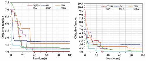
As can be seen from Figure 8, compared with the GA and PSO, the GA and PSO converge faster in the first 10 generations or so, but after 10 generations, the CQSSA continues to converge, while the GA and PSO converge significantly slower and fall into local optimal solutions that cannot be jumped out. Compared with the SSA, the CSSA converges faster compared with the QSSA, and the convergence effect is obvious in the first 10 generations or so. Compared with the CSSA and QSSA, the CQSSA convergence speed is not much different from both of them, but it can continue to converge in the later stage of the algorithm and calculate to obtain a better-quality solution. Thus, the convergence performance of the CQSSA is better, and solving the E-B&QC model based on the CQSSA is more efficient and leads to a better-quality solution.

Conclusion

An efficient berth-quay crane allocation scheme is very important and practical to solve the problems of port congestion, soaring freight rates, and hard-to-find container spaces brought about by the normalization of the epidemic. In this paper, a new joint berth-quay crane allocation method (E-B&QC-CQSSA) is established based on chaotic perturbation, quantum computing, and the SSA considering the economic cost. The results of the simulation test study with actual port data show that: the E-B&QC model established in this paper can provide different berth quay crane allocation schemes for ports under different working conditions by adjusting the weight coefficients to meet the needs of container ports at different times. The larger the container port and the more complex the loading and unloading operation process, the more obvious the effect of applying the E-B&QC model for logistics optimization of the container port. The CQSSA solution algorithm proposed in this paper addresses the shortcomings of the SSA, based on chaos mapping and quantum theory, and establishes the CQSSA to make up for the shortcomings of the SSA, and applies it to solve the established E-B&QC model, and the comparison of simulation results with other traditional methods shows that the solution algorithm established in this paper obtains a better allocation scheme. It makes the solving process more accurate, stable, and efficient.

In conclusion, this paper proposes a feasible approach, based on the CQSSA solved the E-B&QC model for port schedule. Especially as the size of the port increases, the approach can obtain a better scheduling solution.

However, the berth-crane optimization method proposed in this paper has the following two shortcomings: firstly, the extra waiting time cost coefficient of ships in the E-B&QC model is not yet accurate and needs to be further studied; secondly, meteorological factors such as tides can also have an impact on container port operation costs, which have not yet been considered in this paper.

Disclosure Statement

No potential conflict of interest was reported by the author(s).

Data Availability Statement

All employed data will be made available on reasonable request. http://gkhy.jiujiang.gov.cn/

Additional information

Funding

This work was supported by the National Social Science Foundation of China (21BGL064); Heilongjiang Social Science Fund (20JYB042); National Key Research and Development Program of China (2019YFB1504403); National Natural Science Foundation of China (No. 51509056); and Ministry of Science and Technology, Taiwan (MOST 110-2410-H- 161-001).

References

- Cai, Y., P. Liu, and H. Xiong. 2020. Berth joint scheduling based on quantum genetic hybrid algorithm. Journal of Computer Applications 40 (3):897–674. doi:10.11772/j.1001-9081.2019071242.
- Cho, S. W., H. J. Park, and C. Lee. 2020. An integrated method for berth allocation and quay crane assignment to allow for reassignment of vessels to other terminals. Maritime Economics & Logistics 23 (1):123–53. doi:10.1057/s41278-020-00173-4.
- Jiao, X., F. Zheng, M. Liu, and Y. Xu. 2018. Integrated berth allocation and time-variant quay crane scheduling with tidal impact in approach channel. Discrete Dynamics in Nature and Society 9097047. doi:10.1155/2018/9097047.
- Jiao, X., F. Zheng, Y. Xu, and M. Liu. 2020. Bi-objective optimization simulation of integrated berth and quay crane scheduling considering tidal influence at container terminal. Computer Simulation 37 (2):403–10. doi:10.3969/j.1006-9348.2020.02.082.
- Karam, A., and A. B. Eltawil. 2016. Functional integration approach for the berth allocation, quay crane assignment and specific quay crane assignment problems. Computers & Industrial Engineering 102:458–66. doi:10.1016/j.cie.2016.04.006.
- Kocarev, L., G. Jakimoski, T. Stojanovski, and U. Parlitz. 1998. From chaotic maps to encryption schemes. Proceeding of 1998 IEEE International Symposium on Circuits & Systems, Monterey, CA, USA, May-3 31 June. article number:6021236. 10.1109/ISCAS.1998.698968
- Li, M. W., W. C. Hong, J. Geng, and J. Wang. 2017. Berth and quay crane coordinated scheduling using multi-objective chaos cloud particle swarm optimization algorithm. Neural Computing & Applications 28 (11):3163–82. doi:10.1007/s00521-016-2226-7.
- Li, M. W., W. C. Hong, and H. G. Kang. 2013. Urban traffic flow forecasting using Gauss–SVR with cat mapping, cloud model and PSO hybrid algorithm. Neurocomputing 99:230–40. doi:10.1016/j.neucom.2012.08.002.
- Li, S., and X. Zheng. 2002. Cryptanalysis of a chaotic image encryption method. Proceeding of 2002 IEEE International Symposium on Circuits & Systems, Phoenix-Scottsdale, AZ, USA, 26–29. May. article number:7439462. 10.1109/ISCAS.2002.1011451
- Liu, G., C. Shu, Z. Liang, B. Peng, and L. Cheng. 2021. A modified sparrow search algorithm with application in 3D route planning for UAV. Sensors 21 (4):1224. doi:10.3390/s21041224.
- Liu, J., and Z. Wang. 2021. A hybrid sparrow search algorithm based on constructing similarity. IEEE Access 9:117581–95. doi:10.1109/ACCESS.2021.3106269.
- Liu, Y., J. Wang, and S. Shahbazzade. 2019. The improved AFSA algorithm for the berth allocation and quay crane assignment problem. Cluster Computing 22 (S2):3665–72. doi:10.1007/s10586-018-2216-x.
- Mao, Y., and G. Chen. 2005. Chaos-based image encryption. In Handbook of Geometric Computing, ed., E. B. Corrochano, 231–65. Berlin, Heidelberg: Springer. doi:10.1007/3-540-28247-5_8.
- Mao, Y., G. Chen, and S. Lian. 2004. A novel fast image encryption scheme based on 3D chaotic baker maps. International Journal of Bifurcation & Chaos 14 (10):3613–24. doi:10.1142/S021812740401151X.
- Nepomuceno, E. G., A. M. Lima, J. Arias-García, M. Perc, and R. Repnik. 2019. Minimal digital chaotic system. Chaos, Solitons, and Fractals 120:62–66. doi:10.1016/j.chaos.2019.01.019.
- Ouyang, C., D. Zhu, and Y. Qiu. 2021. Lens learning sparrow search algorithm[J]. Mathematical Problems in Engineering 9935090. doi:10.1155/2021/9935090.
- Rodrigues, F., and A. Agra. 2021. An exact robust approach for the integrated berth allocation and quay crane scheduling problem under uncertain arrival times. European Journal of Operational Research 295 (2):499–516. doi:10.1016/j.ejor.2021.03.016.
- Sang, T., R. Wang, and Y. Yan. 2001. Generating binary Bernoulli sequences based on a class of even-symmetric chaotic maps. IEEE Transactions on Communications 49 (4):620–23. doi:10.1109/26.917768.
- Song W, S. Liu, X. Wang, and W. Wu. 2020. An improved sparrow search algorithm. Proceeding of 2020 IEEE International Conference on Parallel & Distributed Processing with Applications, Big Data & Cloud Computing, Sustainable Computing & Communications, Social Computing & Networking, Exeter, United Kingdom, 17–19 December 2020, Article number, 20800453. doi:10.1109/ISPA-BDCloud-SocialCom-SustainCom51426.2020.00093
- Thanos, E., T. Toffolo, H. G. Santos, W. Vancroonenburg, and G. V. Berghe. 2021. The tactical berth allocation problem with time-variant specific quay crane assignments. Computers & Industrial Engineering 155:107168. doi:10.1016/j.cie.2021.107168.
- Tian, X., and Q. Meng. 2018. Study on coordinated scheduling of berths, quay cranes and harbor trucks at container terminals. Logistics Technology 37:32–36. doi:10.3969/j.1005-152X.2018.03.008.
- Vrakas, G., C. Chan, and V. V. Thai. 2021. The effects of evolving port technology and process optimisation on operational performance: the case study of an Australian container terminal operator. The Asian Journal of Shipping and Logistics 37 (4):281–90. doi:10.1016/j.ajsl.2020.04.001.
- Wang, P., Y. Zhang, and H. Yang. 2021. Research on economic optimization of microgrid cluster based on chaos sparrow search algorithm. Computational Intelligence and Neuroscience 2021:5556780. doi:10.1155/2021/5556780.
- Wu, E., and J. Zhu. 2021. Integrated scheduling for berth and quay crane in automated container terminals based on proactive-reactive method. International Core Journal of Engineering 7:60–70. doi:10.6919/ICJE.202108_7(8).0010.
- Xue J, B. Shen, and J. Xue. 2020. A novel swarm intelligence optimization approach: Sparrow search algorithm. Systems Science & Control Engineering An Open Access Journal 8 (1):22–34. doi:10.1080/21642583.2019.1708830.
- Yang, J., H. Gao, T. Liu, and W. Liu. 2016. Integrated berth and quay-crane scheduling based on improved genetic algorithm. Journal of Computer Applications 36:3136–40. doi:10.11772/j.1001-9081.2016.11.3136.
- Yang, L., Z. Li, D. Wang, H. Miao, and Z. Wang. 2021. Software defects prediction based on hybrid particle swarm optimization and sparrow search algorithm. IEEE Access 9:60865–79. doi:10.1109/ACCESS.2021.3072993.
- Yuan, J., Z. Zhao, Y. Liu, B. He, L. Wang, B. Xie, and Y. Gao. 2021. DMPPT control of photovoltaic microgrid based on improved sparrow search algorithm. IEEE Access 9:16623–29. doi:10.1109/ACCESS.2021.3052960.
- Zhang, C., and S. Ding. 2021. A stochastic configuration network based on chaotic sparrow search algorithm. Knowledge-Based Systems 220 (10):106924. doi:10.1016/j.knosys.2021.106924.