A Deep Learning Approach for Classification of Dentinal Tubule Occlusions

ABSTRACT

This study aimed to develop a novel deep learning model for reliable quantification of dentinal tubule occlusions instead of manual assessment techniques, and the performance of the model was compared to other methods in the literature. Ninety-six dentin samples were cut and prepared with desensitizing agents to occlude dentinal tubules on different levels. After obtaining images via scanning electron microscope (SEM), 2793 single dentinal tubule images with 48 × 48 resolution were segmented and labeled. Data augmentation techniques were applied for improvement in the learning rate. The augmented data having a total of 10700 images belonging to five classes were used as the network training dataset. The proposed convolutional neural network (CNN) is a class of deep learning model and was able to classify the degree of dentinal tubule occlusions into five classes with an overall accuracy rate of 90.24%. This paper primarily focuses on developing a CNN architecture for detecting the level of dentin tubule occlusions imaged by SEM. The results showed that the proposed CNN architecture is an immensely successful alternative and allowed for objective and automatic classification of segmented dentinal tubule images.

Introduction

Dentine is capped and protected by hard-calcified tissue, enamel. The damage, wear, or decay of enamel tissue cannot regenerate itself because it does not contain any living cells. Chronic trauma from tooth brushing, parafunctional habits, periodontal diseases, and acidic dietary components causes weakened and degraded enamel (Miglani, Aggarwal, and Ahuja 2010). Thus, it can no longer protect the sensitive dentine underneath and leads to pain and sensitivity.

Dentine hypersensitivity (DH) has been defined as a short, sharp pain when the dentinal tubules of a vital tooth are exposed to thermal, evaporative, tactile osmotic, and/or chemical stimuli that cannot be described by any other dental defect or pathology (Addy 2002). The most widely accepted theory for pain mechanism in DH was proposed by Brännström, Lindén, and Aström (1967). According to this hydrodynamic theory, exposed dentinal tubules to the oral environment under certain stimuli allow the movement of tubule fluid, which indirectly stimulates the extremities of pulp nerves and causes DH.

The prevalence of DH was reported as 41.9% for seven countries; thus, patient preventive therapies and clinical management of DH is an important area (Nicola Xania West et al. 2013). A broad range of oral care products with various active agents are available for home or professional use (Addy 2005), and there is no consensus has been reached for the treatment of DH (Costa et al. 2014). Two primary strategies used in the treatment process of DH: blocking neural activity at the pulpal tissue and physical occlusion of dentinal tubules. The first nerve desensitization strategy uses potassium-based therapy to interfere with neural transmission. The second DH treatment approach includes physical occlusion and/or sealing of dentinal tubules, thus decreasing the fluid flow within dentinal tubules (Miglani, Aggarwal, and Ahuja 2010). Theoretically, a decrease in dentine permeability (DP) is considered useful for DH treatment (Costa et al. 2014).

Counting and evaluating dentinal tubule occlusions on SEM images has been employed in many studies for a statistical measure of DP (Jones et al. 2015; Nicola X. West et al. 2018). It is impractical and time-consuming to count and grade dentinal tubules manually, so computer-aided analysis is crucial to avoid wrong interpretations and measurements. Automated analysis of dentinal tubule occlusions is one of the less frequently studied topics, although digital image processing techniques and machine learning methods have generated very successful results in various branches of medicine (Cireşan et al. 2013; Yang et al. 2016).

In one of the experimental studies in the literature that uses digital image processing technique, Ciocca et al. (2007) presented an analysis program to count the number of dentinal tubules and compute the area. The program extracts contours and analyses SEM images. The program mainly includes the following steps: extraction of images, noise removal, histogram equalization, enhancing contrast, counting tubule numbers, and computing the intended area in µm (Addy 2002; Ciocca et al. 2007). Olley et al. (2014) developed a computer-assisted analysis program for the quantification of patent dentinal tubules on tandem scanning microscopy (TSM) and SEM images. Their algorithm counts any circular patent dentinal tubules with a greater diameter than 0.83 µm. The correlation value of the patent tubule number between computer analysis and expert was found (≥0.8) on SEM and TSM images.

As can be seen, the studies were mostly concentrated on counting the number of tubules or calculating tubule areas. There is no doubt that automatic classification would ease the process of labeling thousands of dentin tubule images for investigations about DH.

The use of artificial intelligence on images used in studies in dentistry and medicine has increased in recent years (Badrigilan et al. 2021; Fourcade and Khonsari 2019; Takada 2016). To the authors’ best knowledge, no studies were found utilizing Deep Learning (DL) algorithms about the classification of dentinal tubule occlusions on SEM images. On the contrary, it needs more effort to develop robust and effective methods to overcome time-consuming processes, manual counting errors, and classification variabilities. In particular, DL algorithms, in particular, CNN, can negate the disadvantages of conventional analysis methods and offer high success rates for image classification (Ker et al. 2017). The idea behind this method was firstly introduced by Fukushima, Miyake, and Ito (1983); then, the emergence of CNN for deep learning was started with the demonstration of LeNet-5 by LeCun et al. (1998). In 2012, AlexNet architecture achieved great success by scaling the insights of LeNet into a much sizable neural network in the ImageNet competition (Alex, Sutskever, and Hinton 2012). Accordingly, the improved architecture allows learning much more complex objects and object hierarchies with the help of computing power.

The study presented herein aims to develop a digital image analysis system by bringing usage of the CNN method on segmented dentinal tubule images. The study quantifies and classifies segmented dentinal tubule images into five different occlusion levels by developed CNN model as a novel method.

Materials and Methods

Sample Preparation

The study was approved by the Ethics Committee of Karabuk University (2021/531, 4/8/2021) and the patients submitted a signed informed consent prior to their inclusion in the study. Total of 96 third molar teeth, which were extracted for periodontal or orthodontic reasons, were included for the study. All of them were free of caries and restorations. Just after the extraction, teeth were rinsed off all organic matter in a fume hood and stored in an aqueous solution of 0.15 M NaCl at 4°C for two weeks.

After coronal sectioning, dentin disc extraction was made perpendicular to the long axis of the tooth using a water-cooled, low-wheel-speed adjusted (Secotom-50, Struers, Copenhagen, Denmark) cutting device with a diamond disc (Ø 125 mm × 0.35 mm × 12.7 mm, 33°C) (Figure 1). The dentin discs were kept apart from coronal enamel and pulp horns and had a thickness of 1.05 mm ±0.18. All dentin disc samples were subjected to a metallographic procedure to obtain a uniform surface, grinding with SiC paper [200, 300, 400, and 600 grits] (Metkon Discs, Metkon, Bursa, Turkey) and polishing with 3 µm diamond paste.

Figure 1. Extraction of dentin discs from a human third molar tooth.

Following the metallographic procedure, dentine discs were rinsed with distilled water and sonicated for 20 minutes to eliminate foreign substances. Then, the dentine discs were etched in a petri dish with 37.5% orthophosphoric acid solution (i-dental; Medicinos Linjia UAB, Lithuania) for 30 seconds to open the dentinal tubules. After opening the dentinal tubules, the discs were rinsed with distilled water again and sonicated using an ultrasonic cleaner (Ultrasonic Cleaner, Alex Machine, Istanbul, Turkey) for 10 min to remove orthophosphoric acid residue.

Application of Desensitizing Agents

Desensitizing agents used in this study are for the management of dentin hypersensitivity by occluding patent dentinal tubules. Dentinal discs were divided into six groups, each having 16 discs. Following the manufacturer’s directions, the first two groups of discs were applied with an in-office product Teethmate® and SmartProtect®. The third, fourth, and fifth groups were applied with Novamin®, arginine-calcium carbonate, and 1.4% potassium-oxalate. The sixth group was considered as a control, and samples in this group were only kept in NaCl solution without being treated with any agents. All the samples were placed in a 6% C6H8O7 – citric acid (pH = 2.1) solution in a petri dish for a minute and then rinsed in saline for 2 min. Each applied agent had various effects on occluding dentinal tubules (Cummins 2010; Pradeep and Sharma 2010). Creating different levels of dentinal occlusion provided more discriminative information for the dataset.

SEM Image Analysis

After applying the test agents, dentine discs were sputter-coated with a layer of Au-Pd alloy (Q150R Rotary-Pumped Sputter Coater, Quorum, East Sussex, United Kingdom) in a vacuum environment to improve imaging of the samples. The images were obtained by SEM (Carl Zeiss Ultra Plus Gemini FE-SEM, Zeiss, Oberkochen, Germany). Surface morphology was evaluated with the acquired images were taken on a random zone with 3000x magnification. Since each test agent has a different occlusion effect on dentinal tubules, collected images had a more significant number of useful features for the created neural network.

Validation

2793 individual dentin tubule images obtained from dentin discs were saved in 48 × 48 resolution in grayscale form. As previous research suggests that dentinal tubule occlusions ranked using a visual scoring index of 1 to 5 (Chen et al. 2015; Ryan C. Olley et al. 2012; Kunam et al. 2016). According to the scoring index: (L1) unoccluded (0%, no tubule occlusion); (L2) mostly unoccluded (<25% of tubules occluded); (L3) partially occluded (25–<50% of tubules occluded); (L4) mostly occluded (50–<100% of tubules occluded); (L5) occluded (100% of tubules occluded).

Afterward, dentinal tubule occlusions within all the groups were assessed into five classes by two independent and blinded experts. Cohen’s kappa test was carried out to measure agreement between experts qualitatively. Examiners showed that an agreement of >0.80 indicates a strong level of agreement (McHugh 2012). The classes’ data distribution must be balanced to each other to perform a proper classification with deep learning methods. Otherwise, the performance of most standard algorithms significantly reduced to provide accurate classification (Haibo and Garcia 2009). Under-sampling is one of the solutions to overcome this problem. In this study, the images obtained from dentin discs have a high number of L1 and L5 data compared to the other three classes. Therefore, 560 of them were randomly chosen to balance the data count to other classes. L2, L3, and L4ʹs data count of other classes include 558, 558, 559 images, respectively. Then, the dataset was split into training (85%) and test set (15%).

Data Augmentation

Limited datasets are one of the challenges that reduce the generalization performance of deep learning models. When big data is supplied, image analysis tasks with CNN are very powerful, especially in the medical field (Esteva et al. 2017; Gulshan et al. 2016). Data augmentation is one of the techniques that help to solve this problem. In this technique, slightly modified copies of original data were generated to increase the diversity of the training dataset and amount of data. Thus, the model can extract more features and improve the learning rate.

Simple image-based data augmentation generally performs well and increases the performance of computer vision applications (Connor and Khoshgoftaar 2019). In this study, various geometric transformations (Rotation, Shearing, Flipping, Scaling) have been applied to expand the number of dentinal tubule images (Figure 2). A total of 10700 images are obtained by augmentation and used in training the CNN. Sample images of each class and the properties of the generated dataset belonging to each class are given in Table 1.

Table 1. Properties of the generated dataset.

Property\Class	L1	L2	L3	L4	L5	Total
Sample Image
Number of Samples	560	558	558	559	560	2793
Training Set	428	427	427	428	427	2137
Data Augmentation	2140	2140	2140	2140	2140	10700
Validation Set	48	47	47	47	49	237
Test Set	84	84	84	84	84	420
Number of Channels	1
Resolution	48 × 48

Figure 2. Example images of before and after data augmentation process.

Convolutional Neural Networks

The architecture of CNN was biologically inspired by the organization of the Visual Cortex (Fukushima 1988; Hubel and Wiesel 1968). Particularly, the structure of the visual system behaves in such a way as to encode visual relations layer by layer. Each layer gradually represents more specific features (Hubel and Wiesel 1962). CNN is designed to emulate the same organizational behavior. CNN is a type of deep learning model, and they are one of the most powerful tools to do image recognition, classifications, segmentation, and many more tasks (Girshick et al. 2014; Ren et al. 2017; Sermanet et al. 2014). Each input image passes through a series of building blocks to classify relevant objects. Building blocks are the sequence of layers used to assign weights and biases to neurons.

The convolutional layer, non-linearity layer, pooling layer, and fully connected layer are the typical elements of CNN architecture (Albawi, Abed Mohammed, and Al-Zawi 2017). Convolution is the first and fundamental layer that performs feature learning through filter matrices. It is a mathematical operation that takes two inputs as an image matrix and filter. Moving the filter through the entire image will give a convolved feature map. Thus, applying multiple filters produces multiple convolved feature maps. The non-linearity layer comes after the convolution layer for adjusting the output. This layer introduces the network with non-linearity and applies activation functions such as tanh, sigmoid, or Rectified Linear Unit (ReLU). The pooling layer is a down-sampling operation to reduce computational complexity and avoid over-fitting (Albawi, Abed Mohammed, and Al-Zawi 2017). The fully connected layer flattens the values of previous layers by turning them into a vector. Each neuron in one fully connected layer was connected to all neurons in the next layer. Over a series of epochs, CNN tries to learn correct weights for neurons, and the validation test gives an idea about the success of the network.

Proposed Architecture

Adjusting the best performing CNN architecture and optimal neural network hyper-parameters remains empirical. Thus, choosing the best performing CNN for a given problem is quite challenging and directly affects the network’s success. For example, a wider network may lead to more expressive results, but it is much more computationally expensive. On the other hand, if the network is too shallow, the correct features may not be learned. To keep the computational burden acceptable, the number of convolution layers, length of strides, and size of filters taken into consideration while designing the network. In this manner, various experiments have been conducted by tweaking hyper-parameters to choose the best performing network. The proposed architecture is given in Figure 3.

Figure 3. The proposed CNN architecture.

In the first and second convolution layers, 48 × 48 single-channel grayscale images were scanned with 16 different 3 × 3 kernels and a stride of 1 to obtain a high receptive field. Small kernel size with more layers allows mapping more complex features than fewer layers with a larger kernel. Padding value was determined as same for whole convolutional layers to extract more information that lies on the edge of the images. Then, the ReLU activation function is applied after all the convolution layers and given in Equation. 1(1) $\mathrm{f}\left(\mathrm{x}\right)=\mathrm{m}\mathrm{a}\mathrm{x}\left(0,\mathrm{x}\right)\left\{{ }_{0\mathrm{o}\mathrm{t}\mathrm{h}\mathrm{e}\mathrm{r}\mathrm{w}\mathrm{i}\mathrm{s}\mathrm{e}.}^{\mathrm{i}\mathrm{f}\mathrm{x}>0,}\right.$(1) .

(1) $\mathrm{f}\left(\mathrm{x}\right)=\mathrm{m}\mathrm{a}\mathrm{x}\left(0,\mathrm{x}\right)\left\{{ }_{0\mathrm{o}\mathrm{t}\mathrm{h}\mathrm{e}\mathrm{r}\mathrm{w}\mathrm{i}\mathrm{s}\mathrm{e}.}^{\mathrm{i}\mathrm{f}\mathrm{x}>0,}\right.$(1)

After the layers of convolution operation, the max pool layer summarized activation maps, keeping the number of parameters low. Thus, 16 different 16 × 16 feature maps were obtained, and the dropout layer with a rate of 0.2 comes to prevent overfitting by randomly activating and deactivating selected neurons. Just as the beginning of the proposed architecture, the fifth and sixth layers includes similar convolution operation with a kernel size of 5 × 5 and ReLU activation function. This operation provides a constant number of parameters while increasing the receptive field and the number of obtained features. Moreover, repeated application of convolution operation has been used in many state-of-the-art models, such as VGG16 (Simonyan and Zisserman 2015) and AlexNet (Alex, Sutskever, and Hinton 2012).

The seventh layer includes the max pool operation, and the size of the feature maps was reduced again. Dropout was applied with a rate of 0.8 after the second max pool layer. In the classification part of the architecture, the resulting kernels were flattened and connected to 256 fully connected neurons with a dropout rate of 0.5 and then connected to five neurons to classify five different occlusion levels. Details of the proposed structure of the network parameters are given in Table 2.

Table 2. The detail of the proposed CNN architecture trained on 48 × 48 grayscale images.

Layer Type	Kernel	Stride	Padding	Activation	Rate	Output Shape	Parameters
Convolution	3 × 3	1	same	ReLU	-	48 × 48 × 16	160
Convolution	3 × 3	1	same	ReLU	-	48 × 48 × 16	2320
Max-Pooling	3 × 3	3	-	-	-	16 × 16 × 16	-
Dropout	-	-	-	-	0.2	16 × 16 × 16	-
Convolution	5 × 5	1	same	ReLU	-	16 × 16 × 32	12,832
Convolution	5 × 5	1	same	ReLU	-	16 × 16 × 32	25,632
Max-Pooling	2 × 2	2	-	-	-	8 × 8 × 32	-
Dropout	-	-	-	-	0.8	8 × 8 × 32	-
Flatten	-	-	-	-	-	1 × 1 × 2048	-
Fully-Connected	-	-	-	-	-	1 × 1 × 256	524,544
Dropout	-	-	-	-	0.5	1 × 1 × 256	-
Fully-Connected	-	-	-	SoftMax	-	1 × 1 × 5	1285

The optimizer shapes the model into the most accurate possible form by changing the weights and preventing local minimum phenomena. Adaptive Moment Estimation (ADAM) (Kingma and Jimmy 2015) optimizer was used to find global minimum value with a fixed learning rate of 0.001. Since more than two-class label classification is required in the present study, the SoftMax activation function was chosen in the network’s output layer. The formula is given in Equation. 2(2) $\sigma {\left(\hat{\mathbf{x}}\right)}_i=\frac{e^{{\mathrm{x}}_{\mathrm{i}}}}{{\mathrm{\Sigma }}_j{e}^{{\mathrm{x}}_{\mathrm{j}}}}$(2) .

(2) $\sigma {\left(\hat{\mathbf{x}}\right)}_i=\frac{e^{{\mathrm{x}}_{\mathrm{i}}}}{{\mathrm{\Sigma }}_j{e}^{{\mathrm{x}}_{\mathrm{j}}}}$(2)

The function takes an input vector x to calculate normalized probabilities for each class within the range of [0,1]. The elements of an output vector add up to 1, and j represents the class count. In this manner, the predicted class will have the highest probability value out of all the classes. One-hot-encoded target vectors represent the expected multinomial probability for each class (five in this study). The encoded vector takes 1 for the correct label and 0 for other classes. To get the total loss, the error rate between the expected and estimated output was calculated using the cross-entropy function presented in Equation. 3(3) $\mathrm{C}\mathrm{E}=-{\sum }_I{t}_{i}log(\sigma ({\hat{\mathbf{x}}}_i))$(3) . t represents the ground truth vector. The error rate helps to update the network for better estimations.

(3) $\mathrm{C}\mathrm{E}=-{\sum }_I{t}_{i}log(\sigma ({\hat{\mathbf{x}}}_i))$(3)

Batch size is the other hyperparameter used while training the network. This value refers to the number of training images in one each forward/backward iteration. Although a large batch size could lower the loss value, smaller values lead to converging quickly with a noise cost in the training process. The batch size and epoch were defined as 256 and 300, respectively. An epoch refers that the entire dataset is passed both forward and backward one time. After each forward propagation, the total error was calculated for each set, and weight updates are done via backpropagation, and the optimizer tries to minimize the loss until convergence. Besides, the training data set was split randomly in a 90:10 ratio to compose the training and validation dataset. Thus, the network takes 10700 images, in sets of 256, pass through in each epoch for training the model. For the rest of the images, a validation dataset was used to evaluate and pick a model considering the success rate. Different sets of images were used in each epoch by shuffling the training data. The primary purpose behind shuffling is to prevent the network from overfitting and have accurate classification results. The number of obtained trainable parameters is 566,773.

Results

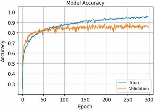
It is commonly accepted that a well-trained network should maximize not only training accuracy but also validation accuracy. If validation accuracy starts to decrease, the trained network is overfitting to the training data meaning that the model loses its generalization capability. Thus, various regularization and normalization techniques are applied to achieve high performance. Figure 4 shows all the training and validation accuracy rates when the network was in the learning process. After the learning phase, the highest validation accuracy was 89.17% at the 256th epoch, chosen as the network’s optimum parameters.

Figure 4. Training and validation accuracy rates.

The network’s effectiveness was studied by consulting the network with test data, and the overall classification accuracy was 90.24%. As can be seen in Figure 5, the confusion matrix visualizes the combinations of actual/predicted classes that were generated to analyze the network’s performance with statistical metrics in terms of sensitivity, specificity, precision, and accuracy. The obtained classification report is given in Table 3.

Table 3. Classification report of the test results.

	Sens.(%)	Spec.(%)	Prec.(%)	Acc.(%)
L1	96.43	99.00	96.43	98.44
L2	88.10	97.44	90.24	95.47
L3	83.33	95.37	82.35	92.89
L4	86.90	96.53	86.90	94.51
L5	96.43	98.68	95.29	98.19

Figure 5. Confusion matrix with and without normalization.

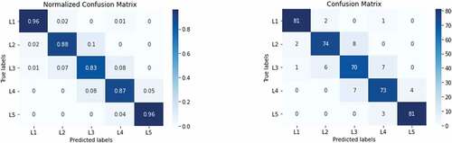
The results were demonstrated that the model is robust and performs well for classification tasks. As confirmed by the confusion matrix results, the false predictions that the model produced mostly belongs to the L3 class. A total of 41 out of 420 dentinal tubule images were wrongly classified. However, when these misclassified images were investigated in detail, they are relatively close to the predicted class; even experts may fail to spot the difference.

Discussion

Producing accurate, repeatable, and consistent classification results are crucial for the reliability of the statistical analysis. Image processing techniques and machine learning algorithms can also be useful for assessing dentinal tubules, but success rates highly depend on the chosen parameters. On the other hand, deep learning, especially CNN, showed excellent performance for classification tasks.

In this study, different desensitizers are applied to dentin discs to include different levels of dentin occlusion images. Data augmentation provided variation in the training data. Image variability not only increases learning performance but also enhances the generalization capability of the network. Since each pixel includes essential features, the proposed CNN architecture included four layers of convolution operation to benefit from every feature as much as possible. These features on the images were the most crucial factor that affects the discrimination among the classes, thus the success rate. However, the success rate could only reach a certain extent because the data augmentation technique produces new data by applying various transformations to the original images. The test dataset, including all classes of dentinal tubule images, was classified into five classes with 90.24% accuracy. Since these images are not seen by the network before, it gives objective results about the classification.

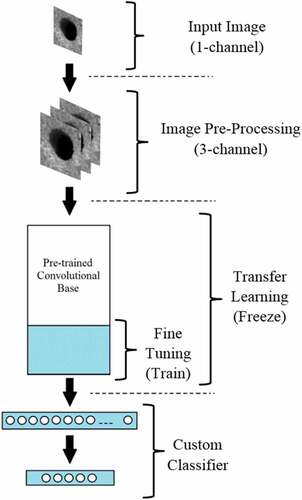
Empty (L1) or fully occluded (L5) dentin tubules were easier to predict than the other three classes. As shown in Figure 5, the confusion matrix shows that L1 and L5 classes’ performances were higher than others. On the other hand, mostly unoccluded (L2) partially occluded (L3), and mostly occluded (L4) classes were difficult to separate from each other because images in neighbor classes were very similar. Therefore, training with a higher number of original data with more discriminative features would help increase each class’s success rate. When a given dataset is small, Transfer Learning (TL) methods are useful and can effectively adapt new data with high success rates (Tajbakhsh et al. 2016). In TL, gained knowledge from a previous task is reused for solving a different but related custom problem. Weight values of the convolutional layers are preserved in the feature extraction phase and linked to a modified number of output layers to classify a new dataset. Thus, obtained weights and previously learned feature extraction capability from a different dataset could be transferred to a new task. On the other hand, Fine Tuning (FT) is an approach to the TL method. In this method, some of the layers or the entire convolutional layers are trained again, and weights of the unfrozen layers are updated in each epoch to better adapt the network to the new dataset.

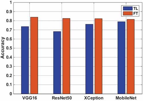
In this manner, four pre-trained models, VGG16 (Simonyan and Zisserman 2015), ResNet50 (Kaiming et al. 2016), XCeption (Chollet 2017), and MobileNet (Howard et al. 2017), were performed to examine their performances with the study dataset. Since the layers of given models are arranged for 3-channel images, data in the existing channel was reproduced for the remaining two channels, and the dataset was resized for specified input dimensions. After the preparation of the dataset, two methods were adopted for the application of pre-trained models. ImageNet dataset was used for all the weight initializations of the methods (Deng et al. 2009). In the TL method, all the feature extraction layers were preserved by freezing the convolutional base. The final convolutional layer was then flattened and connected to two dense layers containing 256 and 5 neurons.

In the FT method, initial layers were kept frozen again, but later convolutional layers were included in the training process since they detect more distinguishing features. The final convolutional layer was then flattened and connected to two dense layers containing 256 and 5 neurons again. The overall visualization of both adapted strategies is given in Figure 6.

Figure 6. Adapted strategies for TL and FT applications.

The FT method adapted better to new samples than the TL method because of the increase in trainable layers (Figure 7). The best validation accuracy of 84.16% was obtained from VGG-16 architecture with FT. On the other hand, none of the TL methods could overtake the FT method. Although the FT method achieved higher validation rates, all the results stayed behind the proposed CNN method trained from scratch. The root cause of performance decrease in learning rate can be explained by the inclusion of irrelevant samples from the source dataset, which is also called negative transfer. A decrease in the similarity between the target domain and the ImageNet dataset affected the learning adversely.

Figure 7. Validation rates of TL and FT methods.

Conclusions

Investigations on dentin tubules are crucial for improvements in dental care, and the use of SEM combined with CNN eases the analysis process. Through analyzes carried on dentin tubules, it is possible to inspect the effect of the applied product. In this regard, measuring the occlusion degree of dentin tubules gives essential information about the applied product. Therefore, automatic analysis is a critical requirement in this field to reduce these negative impacts. Image processing techniques can achieve good classification results with correct parameters, but they can easily be affected by impurities or noise on the image resulting in lower accuracy rates. Deep learning, especially CNN, is a perfect fit to overcome the mentioned issues and automate dentinal tubules’ assessment process. Furthermore, automatic analysis benefits from being independent of an examiner while being time-efficient. Since CNN can learn and classify a broad range of data, noisy images can also be classified with high accuracy.

In this study, a novel CNN architecture was presented for the classification of dentinal tubule occlusions. 2793 segmented dentin tubule images split into two parts so that 85% training and 15% testing dataset. The data augmentation technique was applied only to the training dataset to extract more features from each image. After the training process, test data not seen by the network was fed into the trained model, and the overall accuracy was found to be 90.24%. The proposed architecture has shown the ability to capture dentinal tubule occlusions’ specific features and classify them accordingly. The overall proposed method is practical to use in terms of time efficiency, objectiveness, and high classification accuracy rates.

Disclosure Statement

No potential conflict of interest was reported by the author(s).

References

- Addy, M. 2002. Dentine hypersensitivity: New perspectives on an old problem. International Dental Journal 52 (5):367–2600. doi:10.1002/j.1875-595x.2002.tb00936.x.
- Addy, M. 2005. Tooth brushing, tooth wear and dentine hypersensitivity are they associated? International Dental Journal 55: 261–267 . doi:10.1111/j.1875-595X.2005.tb00063.x.
- Albawi, S., T. Abed Mohammed, and S. Al-Zawi. 2017. “Understanding of a convolutional neural network.” In 2017 International Conference on Engineering and Technology (ICET) , Antalya, Turkey -. 10.1109/ICEngTechnol.2017.8308186.
- Alex, K., I. Sutskever, and G. E. Hinton. 2012. ”ImageNet classification with deep convolutional neural networks.”In 26th Annual Conference on Neural Information Processing Systems 2012, Lake Tahoe, Nevada, USA. 1, 1097–1105 .
- Badrigilan, S., S. Nabavi, A. Ali Abin, N. Rostampour, I. Abedi, A. Shirvani, and M. Ebrahimi Moghaddam. 2021. Deep learning approaches for automated classification and segmentation of head and neck cancers and brain tumors in magnetic resonance images: A meta-analysis study. International Journal of Computer Assisted Radiology and Surgery 16 (4):529–42. doi:10.1007/s11548-021-02326-z.
- Brännström, M., L. A. Lindén, and A. Aström. 1967. The hydrodynamics of the dental tubule and of pulp fluid. A discussion of its significance in relation to dentinal sensitivity. Caries Research 1 (4):4. doi:10.1159/000259530.
- Chen, C. L., A. Parolia, A. Pau, and I. C. Celerino De Moraes Porto. 2015, 1. Comparative evaluation of the effectiveness of desensitizing agents in dentine tubule occlusion using scanning electron microscopy. Australian Dental Journal 60 (1): 65–72. doi:10.1111/adj.12275.
- Chollet, F. 2017. “Xception: Deep learning with depthwise separable convolutions.” In 2017 IEEE Conference on Computer Vision and Pattern Recognition (CVPR), Honolulu, HI, USA ,1800–1807 . doi: 10.1109/CVPR.2017.195.
- Ciocca, L., I. Gallina, E. Navacchia, P. Baldissara, and R. Scotti. 2007. A new method for quantitative analysis of dentinal tubules. Computers in Biology and Medicine 37 (3):3. doi:10.1016/j.compbiomed.2006.01.009.
- Cireşan, D. C., A. Giusti, L. M. Gambardella, and J. Schmidhuber. 2013”Mitosis Detection in Breast Cancer Histology Images with Deep Neural Networks”In Medical Image Computing and Computer-Assisted Intervention – MICCAI 2013, Nagoya, Japan. . Springer. 411–418. doi:10.1007/978-3-642-40763-5_51.
- Connor, S., and T. M. Khoshgoftaar. 2019. A survey on image data augmentation for Deep Learning. Journal of Big Data 6:1. doi:10.1186/s40537-019-0197-0.
- Costa, R. S. A., F. S. Rios, M. S. Moura, J. J. Jardim, M. Maltz, and A. N. Haas. 2014. Prevalence and risk indicators of dentin hypersensitivity in adult and elderly populations from Porto Alegre, Brazil. Journal of Periodontology 85 (9):1247–58. doi:10.1902/jop.2014.130728.
- Cummins, D. 2010. Recent advances in dentin hypersensitivity: Clinically proven treatments for instant and lasting sensitivity relief. American Journal of Dentistry 23: Spec No A:3A–13A .
- Deng, J., W. Dong, R. Socher, L. Li-Jia, L. Kai, and L. Fei-Fei. 2009. ”ImageNet: A large-scale hierarchical image database” In 2009 IEEE Conference on Computer Vision and Pattern Recognition, Miami, FL, USA, 248–255 .doi:10.1109/cvpr.2009.5206848.
- Esteva, A., B. Kuprel, R. A. Novoa, K. Justin, S. M. Swetter, H. M. Blau, and S. Thrun. 2017. Dermatologist-Level classification of skin cancer with deep neural networks. Nature 542 (7639):115–18. doi:10.1038/nature21056.
- Fourcade, A., and R. H. Khonsari. 2019, 4. Deep learning in medical image analysis: A third eye for doctors. Journal of Stomatology, Oral and Maxillofacial Surgery 120 (4): 279–88. doi:10.1016/j.jormas.2019.06.002.
- Fukushima, K., S. Miyake, and T. Ito. 1983. Neocognitron: A neural network model for a mechanism of visual pattern recognition. IEEE Transactions on Systems, Man, and Cybernetics SMC-13 (5):826–34. doi:10.1109/TSMC.1983.6313076.
- Fukushima, K. 1988. Neocognitron: A hierarchical neural network capable of visual pattern recognition. Neural Networks 1 (2):119–30. doi:10.1016/0893-6080(88)90014-7.
- Girshick, R., J. Donahue, T. Darrell, and J. Malik. 2014. “Rich feature hierarchies for accurate object detection and semantic segmentation.” In 2014 IEEE Conference on Computer Vision and Pattern Recognition, Columbus, OH, USA, 580–587 . 10.1109/CVPR.2014.81.
- Gulshan, V., L. Peng, M. Coram, M. C. Stumpe, W. Derek, A. Narayanaswamy, S. Venugopalan, K. Widner, T. Madams, J. Cuadros, et al. 2016 . Development and validation of a deep learning algorithm for detection of diabetic retinopathy in retinal fundus photographs. JAMA - Journal of the American Medical Association 316 22: 2402. 10.1001/jama.2016.17216.
- Haibo, H., and E. A. Garcia. 2009. Learning from imbalanced data. IEEE Transactions on Knowledge and Data Engineering 21 (9):1263–84. doi:10.1109/TKDE.2008.239.
- Howard, A. G., M. Zhu, B. Chen, D. Kalenichenko, W. Wang, T. Weyand, M. Andreetto, and H. Adam. 2017. MobileNets: Efficient convolutional neural networks for mobile vision. CoRR abs/1704.04861 http://arxiv.org/abs/1704.04861.
- Hubel, D. H., and T. N. Wiesel. 1962. Receptive fields, binocular interaction and functional architecture in the cat’s visual cortex. The Journal of Physiology 160 (1):106–54. doi:10.1113/jphysiol.1962.sp006837.
- Hubel, D. H., and T. N. Wiesel. 1968. Receptive fields and functional architecture of monkey striate cortex. The Journal of Physiology 195 (1):215–43. doi:10.1113/jphysiol.1968.sp008455.
- Jones, S. B., C. R. Parkinson, P. Jeffery, M. Davies, E. L. Macdonald, J. Seong, and N. X. West. 2015. A randomised clinical trial investigating calcium sodium phosphosilicate as a dentine mineralising agent in the oral environment. Journal of Dentistry 43 (6):757–64. doi:10.1016/j.jdent.2014.10.005.
- Kaiming, H., X. Zhang, S. Ren, and J. Sun. 2016. “Deep residual learning for image recognition.” In 2016 IEEE Conference on Computer Vision and Pattern Recognition (CVPR), Las Vegas, NV, USA, 770–778 , . doi:10.1109/CVPR.2016.90.
- Ker, J., L. Wang, J. Rao, and T. Lim. 2017. Deep learning applications in medical image analysis. IEEE Access 6:1407–15. doi:10.1109/ACCESS.2017.2788044.
- Kingma, D. P., and B. Jimmy 2015. “Adam: A method for stochastic optimization.” In 3rd International Conference on Learning Representations, ICLR 2015 - Conference Track Proceedings, San Diego, CA, USA.
- Kunam, D., S. Manimaran, V. Sampath, and M. Sekar. 2016. Evaluation of dentinal tubule occlusion and depth of penetration of nano-hydroxyapatite derived from chicken eggshell powder with and without addition of sodium fluoride: An in vitro study. Journal of Conservative Dentistry 19 (3):239–44. doi:10.4103/0972-0707.181940.
- LeCun, Y., L. Bottou, Y. Bengio, and P. Haffner. 1998. Gradient-Based learning applied to document recognition. Proceedings of the IEEE 86 (11):2278–324. doi:10.1109/5.726791.
- McHugh, M. L. 2012. Interrater reliability: The kappa statistic. Biochemistry Medicine 22:3. doi:10.11613/bm.2012.031.
- Miglani, S., V. Aggarwal, and B. Ahuja. 2010. Dentin hypersensitivity: Recent trends in management. Journal of Conservative Dentistry 13 (4):218. doi:10.4103/0972-0707.73385.
- Olley, R. C., P. Pilecki, N. Hughes, P. Jeffery, R. S. Austin, R. Moazzez, and D. Bartlett. 2012. An in situ study investigating dentine tubule occlusion of dentifrices following acid challenge. Journal of Dentistry 40 (7):7. doi:10.1016/j.jdent.2012.03.008.
- Olley, R. C., C. R. Parkinson, R. Wilson, R. Moazzez, and D. Bartlett. 2014. A novel method to quantify dentine tubule occlusion applied to in situ model samples. Caries Research 48 (1):1. doi:10.1159/000354654.
- Pradeep, A. R., and A. Sharma. 2010. Comparison of clinical efficacy of a dentifrice containing calcium sodium phosphosilicate to a dentifrice containing potassium nitrate and to a placebo on dentinal hypersensitivity: A randomized clinical trial. Journal of Periodontology 81 (8):1167–73. doi:10.1902/jop.2010.100056.
- Ren, S., H. Kaiming, R. Girshick, and J. Sun. 2017. Faster R-CNN: towards real-time object detection with region proposal networks. IEEE Transactions on Pattern Analysis and Machine Intelligence 39 (6):6. doi:10.1109/TPAMI.2016.2577031.
- Sermanet, P., D. Eigen, X. Zhang, M. Mathieu, R. Fergus, and Y. LeCun. 2014. “Overfeat: Integrated recognition, localization and detection using convolutional networks.” In 2nd International Conference on Learning Representations, ICLR 2014 - Conference Track Proceedings, Banff, Alberta, Canada.
- Simonyan, K., and A. Zisserman. 2015. “Very deep convolutional networks for large-scale image recognition.” In 3rd International Conference on Learning Representations, ICLR 2015 - Conference Track Proceedings, San Diego, CA, USA.
- Tajbakhsh, N., J. Y. Shin, S. R. Gurudu, R. Todd Hurst, C. B. Kendall, M. B. Gotway, and J. Liang. 2016. Convolutional neural networks for medical image analysis: Full training or fine tuning? IEEE Transactions on Medical Imaging 35 (5):1299–312. doi:10.1109/TMI.2016.2535302.
- Takada, K. 2016. Artificial intelligence expert systems with neural network machine learning may assist decision-making for extractions in orthodontic treatment planning. Journal of Evidence-Based Dental Practice 16 (3):190–92. doi:10.1016/j.jebdp.2016.07.002.
- West, N. X., M. Sanz, A. Lussi, D. Bartlett, P. Bouchard, and D. Bourgeois. 2013 . Prevalence of dentine hypersensitivity and study of associated factors: A European population-based cross-sectional study. Journal of Dentistry 41 (10): 841–51. doi:10.1016/j.jdent.2013.07.017.
- West, N. X., J. Seong, N. Hellin, E. L. Macdonald, S. B. Jones, and J. E. Creeth. 2018. Assessment of tubule occlusion properties of an experimental stannous fluoride toothpaste: A randomised clinical in situ study. Journal of Dentistry 76:125–31. doi:10.1016/j.jdent.2018.07.001.
- Yang, X., S. Yong Yeo, J. Mei Hong, S. Thai Wong, W. Teng Tang, W. Zhen Zhou, G. Lee, et al. 2016. “A deep learning approach for tumor tissue image classification.” In 12th IASTED International Conference on Biomedical Engineering, BioMed 2016, Innsbruck, Austria. doi: 10.2316/P.2016.832-025.